Analysis of Bifurcations in a Power System Model with Excitation Limits

Abstract

This paper studies bifurcations in a three node power system when excitation limits are considered. This is done by approximating the limiter by a smooth function to facilitate bifurcation analysis. Spectacular qualitative changes in the system behavior induced by the limiter are illustrated by two case studies. Period doubling bifurcations and multiple attractors are shown to result due to the limiter. Detailed numerical simulations are presented to verify the results and illustrate the nature of the attractors and solutions involved.

1 Introduction

Chaos in simple power system models has been studied extensively in recent papers. In Abed et al., [1993], Tan et al., [1993], bifurcations and chaos in a three node power system with a dynamic load model were studied using a classical model for the generator. In Rajesh & Padiyar [1999], the authors studied dynamic bifurcations in a similar system and reported the existence of chaos even with detailed models. However, in Rajesh & Padiyar [1999], it was observed that the field voltage assumed unrealistic values at the onset of chaos owing to the unmodeled effect of excitation limits. Though a limiter is fairly easy to model for simulation purposes, the effect of a limiter on dynamic bifurcations has been poorly understood because bifurcation analysis demands smoothness of the functions describing the model. Limit induced chaotic behavior in a Single Machine Infinite Bus system was studied in Ji and Venkatasubramanian [1996] by extensive numerical simulations. In this paper, we approximate the limiter by a smooth function to facilitate bifurcation analysis and study the changes which arise on it’s consideration. The rest of the paper is organized as follows. Section 2 deals with the modeling of the system along with the limiter. Section 3 presents the results of a bifurcation analysis. Section 4 contains the discussions and Sec. 5, the conclusions.

2 System Modeling

The system as considered in Rajesh & Padiyar [1999] is shown in Fig. 1. By a suitable choice of line impedances, we might regard the system as one of a generator supplying power to a local load which in turn is connected to a remote system modeled as an infinite bus. For the general reader’s convenience, a brief explanation of the terms d-q and D-Q axis is provided here. The modeling and analysis of three phase synchronous machines is complicated by the fact that the basic machine equations are time varying. This is circumvented by the use of Park’s transformation which transforms the time varying machine equations in to a time invariant set. The three phase stator quantities (like voltage, current and flux), when transformed in to Park’s frame yield the corresponding d-q-o variables. When a generator is described in the d-q frame, then naturally the external network connected to it should also be described in the same reference frame. However, the non-uniqueness of Park’s transformation (each generator has it’s own d-q components) prevents us from doing so. In order to transform the entire network using a single tranformation with reference to a common reference frame, the Kron’s transformation where the variables are denoted by D-Q-O are used. For a complete , detailed and clear exposition of these concepts in power system modeling, the reader is refered to Padiyar [1996].

Figure 1: The System

2.1 Generator Model

Rotor Equations
The rotor mechanical equations for the generator as given by the swing equations are,

$$\dot{\delta}=\omega_{B}s_{m}$$ (1)

$$\dot{s_{m}}=\frac{-ds_{m}+P_{m}-P_{g}}{2H}$$ (2)

where $d$ is the damping factor in per unit, $\omega_{B}$ is the system frequency in rad/s, $P_{m}$ is the input power to the generator and $s_{m}$, the generator slip defined by

$$s_{m}=\frac{\omega-\omega_{B}}{\omega_{B}}$$ (3)

Two electrical circuits are considered on the rotor, the field winding on the d-axis and one damper winding on the q-axis. The resulting equations are,

$$\dot{E^{\prime}_{q}}=\frac{-E^{\prime}_{q}+(x_{d}-x_{d}^{\prime})i_{d}+E_{fd}}{T^{\prime}_{do}}$$ (4)

$$\dot{E^{\prime}_{d}}=\frac{-E^{\prime}_{d}-(x_{q}-x^{\prime}_{q})i_{q}}{T^{\prime}_{qo}}$$ (5)

The power delivered by the generator $P_{g}$ can be expressed as

$$P_{g}=E^{\prime}_{q}i_{q}+E^{\prime}_{d}i_{d}+(x^{\prime}_{d}-x^{\prime}_{q})i_{d}i_{q}$$ (6)

Stator Equations
Neglecting stator transients and the stator resistance, we have the following algebraic equations

$$E^{\prime}_{q}+x^{\prime}_{d}i_{d}=v_{q}$$ (7)

$$E^{\prime}_{d}-x^{\prime}_{q}i_{q}=v_{d}$$ (8)

2.2 Excitation System

The excitation system for the generator is represented by a single time constant high gain AVR and the limiter as shown in Fig. 2.

Figure 2: Excitation System

The equation for this excitation system is given by

$$\dot{E}_{fdx}=\frac{-E_{fdx}+K_{A}(V_{ref}-V_{t})}{T_{A}}$$ (9)

$$E_{fd}=E_{fdx}\;if\;E_{fd}^{min}<E_{fdx}<E_{fd}^{max}$$ (10)

$$=E_{fd}^{min}\;if\;E_{fdx}<E_{fd}^{min}$$

$$=E_{fd}^{max}\;if\;E_{fdx}>E_{fd}^{max}$$

The limiter shown in Fig. 2 and defined by Eq. 10 is a soft or windup limiter. This limiter model cannot be directly used for bifurcation studies. An approximate model where the limiter is described by a smooth function is given below (see Fig. 3). Here, we consider symmetric limits i.e. $|E_{fd}^{max}|\;=\;|E_{fd}^{min}|\;=\;E_{fdl}$

$$E_{fd}\;=\;f_{lim}(E_{fdx})\;=\frac{2E_{fdl}}{\pi}tan^{-1}(aE_{fdx}\;exp(bE^{2}_{fdx}))$$ (11)

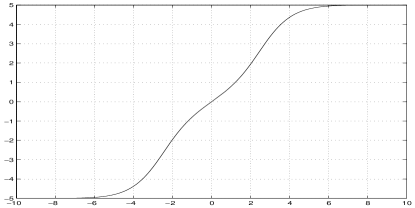
Figure 3: The function representing the limiter

Remarks
Such an approximation amounts to perturbing the vector field slightly and hence the equilibrium structure of the system will also be slightly perturbed. So in our studies, the focus will be on how the limiter influences non-stationary solutions and their bifurcations.

2.3 Load Model

A dynamic load model as in Abed [1993] is used along with a constant power load $(P_{ld},Q_{ld})$ in parallel with it. Thus, the real and reactive load powers are specified by the following equations.

$$P = P_{ld}+P_{o}+p_{1}\dot{\delta_{L}}+p_{2}\dot{V_{L}}+p_{3}V_{L}$$ (12)

$$Q = Q_{ld}+Q_{o}+q_{1}\dot{\delta_{L}}+q_{2}V_{L}+q_{3}V_{L}^{2}$$ (13)

2.4 Network Model

With the notation defined in Fig. 1, we can write the network equation in the D-Q reference frame as,

$$\hat{E_{b}}+\frac{\hat{i_{3}}}{\hat{Y_{3}}}=\hat{V_{t}}$$ (14)

$$\hat{V_{L}}+\frac{\hat{i_{1}}}{\hat{Y_{1}}}=\hat{V_{t}}$$ (15)

Further,

$$\hat{V_{t}}\;\;\;=(v_{q}+jv_{d})e^{j\delta}$$ (16)

$$\hat{i}\;\;\;=\;\;\;(i_{q}+ji_{d})e^{j\delta}\;\;\;=\;\;\;\hat{i_{1}}\;\;\;+\;\;\;\hat{i_{3}}$$ (17)

$$\hat{Y}=Y\angle{\phi}=\hat{Y_{1}}+\hat{Y_{3}}$$ (18)

From Eqs., (14) to (18) we can write,

$$(v_{q}+jv_{d})=\frac{A_{1}+B_{1}}{Y}$$ (19)

where $A_{1}=E_{b}Y_{3}e^{-j(\delta+\phi-\phi_{3})}+Y_{1}V_{L}e^{j(\delta_{L}-\delta-\phi+\phi_{1})}$
and $B_{1}=(i_{q}+ji_{d})e^{-j\phi}$
Defining,

$$a=E_{b}Y_{3}cos(\delta+\phi-\phi_{3})+Y_{1}V_{L}cos(\delta_{L}-\delta-\phi+\phi_{1})$$ (20)

$$b=-E_{b}Y_{3}sin(\delta+\phi-\phi_{3})+Y_{1}V_{L}sin(\delta_{L}-\delta-\phi+\phi_{1})$$ (21)

permits us to write,

$$i_{q}cos(\phi)+i_{d}sin(\phi)=Yv_{q}-a$$ (22)

$$i_{d}cos(\phi)-i_{q}sin(\phi)=Yv_{d}-b$$ (23)

2.5 Derivation of the System Model

Substituting for $v_{d}$ and $v_{q}$ from the stator algebraic equations (7) and (8), we have,

$$\left[\begin{array}[]{cc}cos(\phi)&(sin(\phi)-Yx^{\prime}_{d})\\ -(sin(\phi)-Yx^{\prime}_{q})&cos(\phi)\end{array}\right]\left[\begin{array}[]{c}i_{q}\\ i_{d}\end{array}\right]=\left[\begin{array}[]{c}Y_{a}\\ Y_{b}\end{array}\right]$$ (30)

where   $Y_{a}=(YE^{\prime}_{q}-a)$
and     $Y_{b}=(YE^{\prime}_{d}-b)$

From Eq. (24), we can solve for the currents $i_{d},\;i_{q}$ and subsequently solve for $v_{d}\;$and$\;v_{q}$ from the stator algebraic equations. Further, from Eq. (16) we get,

$$|{\hat{V_{t}}}|=\sqrt{(v_{q}^{2}+v_{d}^{2})}$$ (31)

$$\theta=\delta+tan^{-1}({\frac{v_{d}}{v_{q}}})$$ (32)

Defining,

$$r_{1}\;\;\;=\;\;\;\delta_{L}-\theta-\phi_{1}$$ (33)

$$r_{2}\;\;\;=\;\;\;\delta_{L}-\phi_{2}$$ (34)

the power balance equation at bus 2 can be written as,

$$P=V_{t}V_{L}Y_{1}cos(r_{1})-V_{L}^{2}Y_{1}cos(\phi_{1})+E_{b}V_{L}Y_{2}cos(r_{2})$$

$$-V_{L}^{2}Y_{2}cos(\phi_{2})$$ (35)

$$Q=V_{t}V_{L}Y_{1}sin(r_{1})+V_{L}^{2}Y_{1}sin(\phi_{1})+E_{b}V_{L}Y_{2}sin(r_{2})$$

$$+V_{L}^{2}Y_{2}sin(\phi_{2})$$ (36)

Substituting from Eqs., (LABEL:eq:sys-32), (35-36) in Eqs., (1-5) and (12-13), we get

$$\bf\dot{x}=\bf f(\bf x,\lambda)$$ (37)

where $\bf x=\left[\begin{array}[]{ccccccc}\delta&s_{m}&E^{\prime}_{q}&E^{\prime}_{d}&E_{fdx}&\delta_{L}&V_{L}\end{array}\right]^{T}$ and $\lambda$ is a bifurcation parameter. As a simplification, we shall also consider the system described the One Axis Model for the generator as the effect of the limiter on this case is interesting in itself. For this, we neglect the damper winding on the q-axis and in terms of modeling, this is done by omitting $E^{\prime}_{d}$ as a state variable and substituting

$$E^{\prime}_{d}=-(x_{q}-x^{\prime}_{q})i_{q}$$ (38)

in Eqs., (6) and (8). The state space structure remains the same, with the dimension being one less that the previous system. In this case, we have $\bf x=\left[\begin{array}[]{cccccc}\delta&s_{m}&E^{\prime}_{q}&E_{fdx}&\delta_{L}&V_{L}\end{array}\right]^{T}$.

3 Bifurcations

In this section, we illustrate the qualitative differences which arise on consideration of the limiter by studying bifurcations in the associated systems with AUTO97 (Doedel [1997]) a continuation and bifurcation software for ordinary differential equations. The generator input power ($P_{m}$) is a very important parameter in practical power systems operation. This is the parameter which is adjusted or varied by the power system operators (utility) to track the changes and variations in the system load (power demand) so as to maintain a stable operating condition. We hence, consider $P_{m}$ i.e. the input power to the generator as the bifurcation parameter. To describe the types of bifurcations, we shall use the following notations.
SNB: Saddle Node Bifurcation
HB: Hopf Bifurcation
CFB: Cyclic Fold Bifurcation
TR : Torus Bifurcation
PDB : Period Doubling Bifurcation
In all the bifurcation diagrams the state variable $E_{fdx}$ is plotted against the bifurcation parameter. In the case of periodic solutions, we use the maximum value of the variable which is indicated by the circles. Filled circles refer to stable solutions and the unfilled ones, to unstable solutions.

3.1 One Axis Model

Without limiter
From Fig. 4, we note that the stationary solutions undergo four bifurcations labeled as HB¹, HB², HB³ and SNB⁴. For $\lambda<\lambda^{1}$, the equilibrium point is stable, but as $\lambda$ is increased, the stationary point loses its stability at $\lambda$= $\lambda^{1}$ through HB¹. With a further increase in $\lambda$, the stationary point gains stability through HB², i.e. $\lambda$= $\lambda^{2}$. It remains stable until $\lambda$= $\lambda^{3}$, where stability is lost through HB³. Further, SNB⁴ does not influence the stability of the stationary point. Next, we focus on the family of periodic solutions emerging from HB¹. Since HB¹ is supercritical, it gives birth to a family of stable periodic solutions indicated by the filled circles. This periodic solution loses its stability at TR⁵ and with a further increase in $\lambda$, gains it back through TR⁶ and remains stable until TR⁷. Further on, there is no qualitative change in its behavior with TR⁷, CFB⁸ and TR⁹. Next, we find that the branch emerging on continuation of HB² is the same as that from HB¹. On continuation of HB³, we find a family of unstable periodic solutions which gain stability through CFB¹⁰. This stable periodic solution encounters a PDB¹¹ on continuation of which, we find a period doubling cascade accumulating at a critical value of $\lambda^{c}$ =0.931. (which is not shown here) which definitely suggests the onset of chaos. However, what is of interest here, is the behavior of the system after TR⁵. It is clear that a torus bifurcation results in the emergence of quasi-periodic solutions. This is verified by simulation as shown in Fig. 5 which shows the quasi-periodic attractor. The bifurcation points are summarized in Table  1

Table 1: Bifurcation Points (see Fig. 4)

Point	HB1	HB2	HB3	SNB4	TR5	TR6	TR7	CFB8	TR9	CFB10	PDB11
$\lambda$	0.583	1.0746	1.155	1.914	0.812	1.181	1.26	1.293	1.26	0.922	0.9278

Figure 4: $\lambda=P_{m}$, One Axis Model

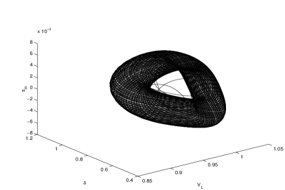
Figure 5: The Quasi-periodic trajectory when $P_{m}=0.83$

With Limiter
From Fig. 6, we observe that the stable operating point loses its stability with HB¹, regains it at HB² and loses it back at HB³ before encountering SNB⁴ which is similar to the case without limiter (see Fig. 4). Note that in Fig. 4, for the static bifurcations HB¹ - SNB⁴, $E_{fdx}<E_{fd}^{max}$ and hence we expect that these bifurcations should occur at the same values even with the limiter. However, this is not the case as seen from Table  2 because of the approximation which shifts the equilibrium structure as mentioned before. HB² and HB³ occur very closely and hence cannot be distinguished in Fig. 6. On continuation of HB¹ which is supercritical, we find that the stable periodic solutions do not undergo any bifurcation. HB² is also supercritical and its continuation yields the same stable periodic set obtained on continuation of HB¹. HB³ is sub-critical and its continuation which yields CFB⁵ where stability is gained for a while before CFB⁶ is however, not shown here. Fig. 7 shows the time domain plot of the load bus voltage for $\lambda=0.86$. The bifurcations are summarized in Table  2.

Table 2: Bifurcation Points (see Fig. 6)

Point	HB1	HB2	HB3	SNB4	CFB5	CFB6
$\lambda$	0.5145	1.1827	1.1857	1.884	1.1284	1.1311

Figure 6: $\lambda=P_{m}$ , One Axis Model with limiter,continuation of HB¹ and HB²

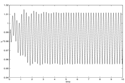
Figure 7: Sustained oscillations of load bus voltage with time when $\lambda=0.86$ with the approximate limiter

3.2 Two Axis model

Without limiter
We let $\lambda=P_{m}$ with reference to Fig. 8. The stationary point undergoes two bifurcations, HB¹ where it loses its stability and SNB² which does not influence the stability further. HB¹ is a supercritical bifurcation and the family of stable periodic solutions from it undergo a period doubling cascade starting with the PDB¹, accumulating at a critical value of $\lambda^{c}=1.315$. The chaotic attractor at $\lambda^{c}$ is shown in Fig. 9 which confirms the chaotic nature. The bifurcation points are summarized in Table 3

Table 3: Bifurcation Points (see Fig. 8)

Point	HB1	SNB2	PDB3	PDB4
$\lambda$	1.2281	1.9607	1.311	1.314

Figure 8: $\lambda=P_{m}$, Two Axis Model

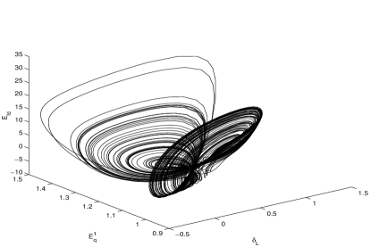
Figure 9: The Chaotic trajectory when $P_{m}$ = 1.315

With Limiter
From Fig. 10, we observe that the stable operating point loses stability at HB¹ and then encounters SNB² (which is not shown here). On continuation of HB¹, which is sub-critical, we find that the unstable periodic solution stabilizes with CFB³. This stable periodic solution undergoes a period doubling cascade initiated at PDB⁴. In Fig. 10,we also show the period doubled solution and its subsequent bifurcation PDB⁵. By numerical simulations, considering both the exact and the function approximation of the limiter, we verify that at $\lambda=1.3$, the system behavior is chaotic. The time domain plots are shown in Figs  11 and  12. The chaotic attractor subject to limits is shown in Fig  13. The bifurcations are summarized in Table  4.

Table 4: Bifurcation Points (see Fig. 10)

Point	HB1	SNB2	CFB3	PDB4	PDB5
$\lambda$	1.2729	1.923	1.2557	1.282	1.2912

Figure 10: $\lambda=P_{m}$, Two Axis Model with limiter

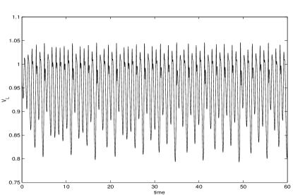
Figure 11: Chaotic oscillations of load bus voltage with time when $\lambda=1.3$ with the approximate limiter

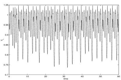
Figure 12: Chaotic oscillations of load bus voltage with time when $\lambda=1.3$ with the exact limiter

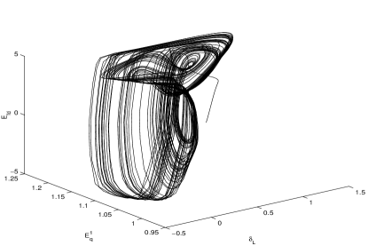
Figure 13: The Chaotic attractor subject to limits when $\lambda=1.3$

4 Discussions

The case studies with two different models were considered solely for illustrating the effect of the limiter on bifurcations in the system which is interesting in it’s own right. The qualitative difference in system dynamics owing to modeling is however not discussed here (see Rajesh and Padiyar [1999] for a discussion). Another aspect worth mentioning is the differences in the bifurcation diagrams in this paper from those in the references. Abed et al consider a simplified generator model (classical model) in which the excitation system is entirely absent and use a slightly different system for the bifurcation studies. In Ji and Venkatasubramanian [1996], a Single Machine Infinite Bus (SMIB) system (which is different from that considered in this paper) wherein the load model is absent, is studied. This paper however, focusses mainly on studying bifurcations and changes which arise on the consideration of excitation limits. When the One axis model is considered without the limiter, we observe stable quasi-periodic trajectories resulting from a TR bifurcation. However, with the limiter, we do not observe any bifurcations of periodic solutions with the result that the entire branch from HB¹ to HB² in Fig. is stable. When the Two axis model is considered without the limiter, we observe chaotic trajectories due to PDBs, which, with the limiter still occur. However, we observe in this case that the system has multiple attractors (see Fig. 10) namely, a stable equilibrium point and a stable periodic solution. Further, we observe that the PDBs in this case occur very close to the boundary of stable fixed point operation. This means that if the system operates close to boundary of stable fixed point operation, and suffers a disturbance with the post-disturbance initial condition belonging to the chaotic region, the system can be easily pushed to the chaotic region. Another interesting aspect seen by comparing Fig. 8 and Fig. 10 is that stable equilibrium points close to the boundary of stable fixed point operation are surrounded by unstable limit cycles which suggests that the region of attraction for the equilibrium points shrinks in the presence of limits.

5 Conclusions

An attempt has been made to analyze bifurcations in the presence of a limiter by approximating the limiter by a smooth function. It is seen that this methodology provides good insight in to studying bifurcations in a system with a soft limiter. The observations in the case studies illustrate in general that, the limiter is capable of inducing spectacular qualitative changes in the system. Developing a formal theory for bifurcations and analyzing the global system dynamics in the presence of limits in the system would be a challenging task for further research in this area.

References

Abed E. H., Wang H. O., Alexander J. C., Hamdan A. M. A. and Lee H. C. [1993] “Dynamic bifurcations in a power system model exhibiting voltage collapse”, Int. J. Bifurcations and Chaos 3 (5), 1169-1176.

Doedel E. J., Fairgrieve T. F., Sanstede B., Champneys A. R., Kuznetsov and Wang X [1997] “AUTO97 : (User’s Manual) continuation and bifurcation software for ordinary differential equations.”

Ji W. and Venkatasubramaian V [1996] “Hard limit induced chaos in a fundamental power system model”, International Journal of Electrical Power and Energy Systems 18 (5), 279-295.

Padiyar K. R. [1996] “Power System Dynamics and Control” John Wiley, Singapore.

Rajesh K. G. and Padiyar K. R. [1999] “Bifurcation analysis of a three node power system with detailed models” International Journal of Electrical Power and Energy Systems 21 375-393.

Tan C. W., Varghese M., Varaiya P. P. and Wu F. W.[1995] “Bifurcation,chaos and voltage collapse in power systems” Proceedings of the IEEE 83 (11) 1484-1496.

Appendix A

• Network parameters.
  $Y_{1}=4.9752,Y_{2}=1.6584,Y_{3}=0,\phi_{1}=\phi_{2}=\phi_{3}=-1.4711,E_{b}=1.0$

• Generator parameters.
  $x_{d}=1.79,\;\;\;x_{q}=1.71,\;\;\;T^{\prime}_{do}=4.3,T^{\prime}_{qo}=0.85,x_{d}^{\prime}=0.169,\newline x_{q}^{\prime}=0.23,H=2.894,w_{b}=377,d=0.05,E_{m}=1.0$

• Load parameters.
  $P_{o}=0.4,\;\;,Q_{o}=0.8\;\;,p_{1}=0.24\;\;,q_{1}=-0.02\;\;,p_{2}=1.7\;\;,q_{2}=-1.866\newline p_{3}=0.2\;\;,q_{3}=1.4\;\;$

• AVR constants
  $K_{A}=200\;\;,T_{A}=0.05$

• Limiter constants $a=0.23\;,\;b=0.1058\;,\;E_{fd}^{max}=5\;,\;E_{fd}^{min}=-5$