Entropy production in diffusion-reaction systems: The reactive random Lorentz gas

Abstract

We report the study of a random Lorentz gas with a reaction of isomerization $A\rightleftharpoons B$ between the two colors of moving particles elastically bouncing on hard disks. The reaction occurs when the moving particles collide on catalytic disks which constitute a fraction of all the disks. Under the dilute-gas conditions, the reaction-diffusion process is ruled by two coupled Boltzmann-Lorentz equations for the distribution functions of the colors. The macroscopic reaction-diffusion equations with cross-diffusion terms induced by the chemical reaction are derived from the kinetic equations. We use a $H$-theorem of the kinetic theory in order to derive a macroscopic entropy depending on the gradients of color densities and which has a non-negative entropy production in agreement with the second law of thermodynamics.

I Introduction

During the last decades, irreversibility and transport properties have been intensively studied in low-dimensional dynamical systems EvHobooks ; GaNi90 ; Ga92 ; ChEyLeSi93 ; Ru96 ; Gabook ; Dobook ; VoTeBr98 ; TeVo00 ; MaTeVo00 ; TaGa00 ; TeVoMa01 ; GiDo99 ; GiDoGa00 ; DoGaGi02 ; GaNiDo02 . It has been shown that the macroscopic transport coefficients can be related to the characteristic quantities of the microscopic dynamics GaNi90 ; Gabook . Moreover, results have also been obtained for the entropy balance in dynamical systems sustaining transport processes of diffusion GiDoGa00 ; DoGaGi02 ; GaNiDo02 , electric conduction VoTeBr98 , cross effects MaTeVo00 ; TaGa00 , and shear viscosity TeVoMa01 ; ViGa03a ; ViGa03b . For these processes, the irreversible entropy production of nonequilibrium thermodynamics could be derived from the underlying microscopic dynamics.

Beside transport, reaction processes have also been investigated from the viewpoint of dynamical systems theory. Reaction-diffusion processes play a crucial role in physico-chemical systems far from the thermodynamic equilibrium and they have been much studied at the macroscopic level of description on the basis of the phenomenological nonequilibrium thermodynamics NiPr77 .

Recently, several microscopic models of reaction-diffusion processes have been introduced and analyzed in order to understand the foundations of the phenomenological assumptions. Multibaker and Lorentz gas models of reaction-diffusion processes were introduced in Refs. GaKl98 ; Ga99 ; footnote1 . In this early version, the reaction was an isomerization $A\rightleftharpoons B$ with unit probability upon the passage of the particle on a catalytic side where the reaction occurs. In Ref. ClGa00 , a spatially periodic reactive Lorentz gas was introduced in which the isomerization $A\rightleftharpoons B$ occurs with a probability $0\leq p_{0}\leq 1$ when the particle collides on catalytic disks. The catalytic disks are few among the disks which compose the Lorentz gas. Spatially periodic Lorentz gas and multibaker models with reaction $A\rightleftharpoons B$ have been studied in detail and their diffusive and reactive modes were constructed together with their dispersion relations ClGa00 ; ClGa02 ; GaCl02 . In this way, the macroscopic reaction-diffusion equations could be derived in a systematic way from the underlying dynamics. The analysis revealed the existence of cross-diffusion effects induced by the reaction. Such cross diffusion is typically overlooked in the phenomenological approach dGM ; KoPr98 . Moreover, the entropy production of the standard phenomenological entropy may be negative because of the cross-diffusion effects. Although this problem only happens for extreme particle densities it nevertheless sheds some doubts on the phenomenological assumptions.

The purpose of the present paper is to clarify these issues and understand the problem of entropy production in such reaction-diffusion systems. For this purpose, we consider a random Lorentz gas with a fraction of catalytic disks where the isomerization $A\rightleftharpoons B$ occurs with a given probability $p_{0}$. The color $A$ or $B$ carried by the moving particle may correspond to the spin of the particle, in which case the catalytic disks model some spin-flipping impurities in the system. For dilute Lorentz gases, we can use kinetic theory and linear Boltzmann-Lorentz equations Be82 ; BoBuSi83 . Thanks to such master equations, we can derive a $H$-theorem which allows us to obtain an expression for the entropy. We prove that the corresponding entropy production is non-negative with respect to the time evolution induced by the macroscopic reaction-diffusion equations.

The plan of the paper is the following. The kinetic equations of the reactive Lorentz gas are introduced in Sec. II where we prove the $H$-theorem. The macroscopic reaction-diffusion equations are derived in Sec. III. The entropy balance is obtained and discussed in Sec. IV. Conclusions are drawn in Sec. V.

II The reactive Lorentz gas

In the random Lorentz gas, fixed circular scatterers correspond to heavy particles and moving point particles to the light ones. The system is defined by the density of the scatterers $n$, their radius $a$, and by the velocity of the light particles $\vec{v}=v(\cos\varphi,\sin\varphi)$, the system being two dimensional. Because the magnitude of the velocities is fixed, the velocity vector can be characterized solely by the angle $\varphi$. Here, we consider a random distribution of the disks with low density $n\ll a^{-2}$.

The reactive Lorentz gas ClGa00 consists of two different types of light particles $A$ and $B$, that have a free flight between the collisions. Some of the fixed scatterers act as catalysts, i.e., if an $A$ particle collides with such a scatterer it becomes a $B$ with the probability $p_{0}$, and vice versa. The catalysts have a density $n_{r}$. The reaction scheme is

$$A+{\rm disk}\, \rightleftharpoons A+{\rm disk}\;,$$ (1)

$$B+{\rm disk}\, \rightleftharpoons B+{\rm disk}\;,$$ (2)

$$A+{\rm catalyst}\, \rightleftharpoons B+{\rm catalyst}\;,\qquad\mbox{with probability}\ p_{0}\;.$$ (3)

The colors can be considered as the two components of a spin one-half carried by the moving particles. The evolution of the system can be characterized by the two distribution functions of the two components $f_{A}(\vec{r},\vec{v})$ and $f_{B}(\vec{r},\vec{v})$. The integral over the velocities of these functions gives the number density at point $\vec{r}$ of each component $A$ or $B$. Having in view that the time evolution of the distribution function $f_{A}$ (resp. $f_{B}$) is also influenced by the presence of the other component $B$ (resp. $A$) that may collide with a catalyst, we obtain the system of equations

$$\partial_{t}f_{A}+\vec{v}\cdot\vec{\nabla}f_{A} = \frac{av(n-p_{0}n_{r})}{2}\int_{-\pi}^{+\pi}d\varphi^{\prime}\left|\sin\frac{\varphi-\varphi^{\prime}}{2}\right|[f_{A}(\vec{r},\varphi^{\prime})-f_{A}(\vec{r},\varphi)]$$ (4)

$$+\frac{avp_{0}n_{r}}{2}\int_{-\pi}^{+\pi}d\varphi^{\prime}\left|\sin\frac{\varphi-\varphi^{\prime}}{2}\right|[f_{B}(\vec{r},\varphi^{\prime})-f_{A}(\vec{r},\varphi)]\;,$$

$$\partial_{t}f_{B}+\vec{v}\cdot\vec{\nabla}f_{B} = \frac{av(n-p_{0}n_{r})}{2}\int_{-\pi}^{+\pi}d\varphi^{\prime}\left|\sin\frac{\varphi-\varphi^{\prime}}{2}\right|[f_{B}(\vec{r},\varphi^{\prime})-f_{B}(\vec{r},\varphi)]$$ (5)

$$+\frac{avp_{0}n_{r}}{2}\int_{-\pi}^{+\pi}d\varphi^{\prime}\left|\sin\frac{\varphi-\varphi^{\prime}}{2}\right|[f_{A}(\vec{r},\varphi^{\prime})-f_{B}(\vec{r},\varphi)]\;.$$

One can observe that the total system of the moving particles $A$ and $B$ follows a diffusive process that can be characterized by the the sum of the distribution functions

$$f\equiv f_{A}+f_{B}\;.$$ (6)

The time evolution of $f$ is given by a linear Boltzmann equation, also known as the Boltzmann-Lorentz equation Be82 ; BoBuSi83 :

$$\partial_{t}f+\vec{v}\cdot\vec{\nabla}f=\frac{avn}{2}\int_{-\pi}^{+\pi}d\varphi^{\prime}\left|\sin\frac{\varphi-\varphi^{\prime}}{2}\right|[f(\vec{r},\varphi^{\prime})-f(\vec{r},\varphi)]\;.$$ (7)

This equation rules the so-called diffusion sector. In order to have the time evolution of both distribution functions, we need a further equation beside Eq. (7).

If we introduce the quantity

$$g\equiv f_{A}-f_{B}\;,$$ (8)

and take the difference of Eqs. (4) and (5), we obtain the equation

$$\partial_{t}g+\vec{v}\cdot\vec{\nabla}g=\frac{av(n-2p_{0}n_{r})}{2}\int_{-\pi}^{+\pi}d\varphi^{\prime}\left|\sin\frac{\varphi-\varphi^{\prime}}{2}\right|[g(\vec{r},\varphi^{\prime})-g(\vec{r},\varphi)]-4avp_{0}n_{r}g(\vec{r},\varphi)\;,$$ (9)

which rules the reaction sector. One can notice that the last equation describes a decay in time of the function $g$ that can be separated from the rest of the solution

$$g(\vec{r},\varphi,t)={\rm e}^{-4avp_{0}n_{r}\,t}h(\vec{r},\varphi)\;.$$ (10)

The equation for $h$ reads

$$\partial_{t}h+\vec{v}\cdot\vec{\nabla}h=\frac{av(n-2p_{0}n_{r})}{2}\int_{-\pi}^{+\pi}d\varphi^{\prime}\left|\sin\frac{\varphi-\varphi^{\prime}}{2}\right|[h(\vec{r},\varphi^{\prime})-h(\vec{r},\varphi)]\;,$$ (11)

which has the same form as Eq. (7).

II.1 $H$-theorem

The Boltzmann entropy of the system of Eqs. (4) and (5) is given by the sum of the entropies of the two components:

$$s=\int d\varphi\;\left(f_{A}\ln\frac{f^{0}}{f_{A}}+f_{B}\ln\frac{f^{0}}{f_{B}}\right)\;,$$ (12)

where Boltzmann’s constant is taken equal to unity, $k_{\rm B}=1$.

Inserting to the integral on the r.h.s. the time evolution Eqs. (4) and (5), we get for the variation of the entropy

$$\partial_{t}s=\int d\varphi\left\{\ln\frac{f^{0}}{{\rm e}f_{A}}\left[-\vec{v}\cdot\vec{\nabla}f_{A}+C_{A}(f_{A},f_{B})\right]+\ln\frac{f^{0}}{{\rm e}f_{B}}\left[-\vec{v}\cdot\vec{\nabla}f_{B}+C_{B}(f_{A},f_{B})\right]\right\}\;,$$ (13)

where the collision integral $C_{A}(f_{A},f_{B})$ has the form

$$C_{A}(f_{A},f_{B})=\int_{-\pi}^{+\pi}d\varphi^{\prime}\left|\sin\frac{\varphi-\varphi^{\prime}}{2}\right|\left[\frac{av(n-p_{0}n_{r})}{2}(f_{A}^{\prime}-f_{A})+\frac{avp_{0}n_{r}}{2}(f_{B}^{\prime}-f_{A})\right]\;,$$ (14)

with the notations:

$$f_{A} = f_{A}(\vec{r},\varphi,t)\;,$$ (15)

$$f_{A}^{\prime} = f_{A}(\vec{r},\varphi^{\prime},t)\;,$$ (16)

$$f_{B} = f_{B}(\vec{r},\varphi,t)\;,$$ (17)

$$f_{B}^{\prime} = f_{B}(\vec{r},\varphi^{\prime},t)\;.$$ (18)

This relation can be written in form of balance dGM

$$\partial_{t}s=-\vec{\nabla}\cdot\vec{J}_{s}+\sigma_{s}\;,$$ (19)

where

$$\vec{J}_{s}=\int d\varphi\;\vec{v}\;\bigg{(}f_{A}\ln\frac{f^{0}}{f_{A}}+f_{B}\ln\frac{f^{0}}{f_{B}}\bigg{)}$$ (20)

is the entropy current and

$$\sigma_{s}=\frac{av}{4}\int d\varphi d\varphi^{\prime}\left|\sin\frac{\varphi-\varphi^{\prime}}{2}\right|\bigg{\{}(n-p_{0}n_{r}) \left[(f_{A}^{\prime}-f_{A})\ln\frac{f_{A}^{\prime}}{f_{A}}+(f_{B}^{\prime}-f_{B})\ln\frac{f_{B}^{\prime}}{f_{B}}\right]$$

$$+p_{0}n_{r} \left[(f_{B}^{\prime}-f_{A})\ln\frac{f_{B}^{\prime}}{f_{A}}+(f_{A}^{\prime}-f_{B})\ln\frac{f_{A}^{\prime}}{f_{B}}\right] \bigg{\}}\geq 0$$ (21)

is the entropy production. One can see on this general form of the entropy production that it is positive definite under the consistency condition that

$$0\leq p_{0}n_{r}\leq n\;.$$ (22)

III Derivation of the macroscopic reaction-diffusion equations

A convenient way to find the solution of Eqs. (7) and (11)

$$\partial_{t}X+\vec{v}\cdot\vec{\nabla}X=\frac{c}{2}\int_{-\pi}^{+\pi}d\varphi^{\prime}\left|\sin\frac{\varphi-\varphi^{\prime}}{2}\right|[X(\vec{r},\varphi^{\prime})-X(\vec{r},\varphi)]\;,$$ (23)

is by writing the distribution functions $X=f$ or $h$ as Fourier series in the velocity angle $\varphi$

$$X(\vec{r},\varphi,t)=\sum_{l=-\infty}^{+\infty}X_{l}(\vec{r},t)\,{\rm e}^{il\varphi}\;.$$ (24)

As a consequence of Eqs. (7) or (11), the Fourier components $X_{l}$ fulfill the following coupled differential equations

$$\partial_{t}X_{l}+v\frac{\partial_{x}-i\partial_{y}}{2}X_{l-1}+v\frac{\partial_{x}+i\partial_{y}}{2}X_{l+1}=\frac{8l^{2}c}{1-4l^{2}}X_{l}\;,$$ (25)

with

$$c=avn\qquad\mbox{for}\quad X=f\;,$$ (26)

and

$$c=av(n-2p_{0}n_{r})\qquad\mbox{for}\quad X=h\;.$$ (27)

The distribution function $X$ being a real function, the Fourier coefficients with negative index are the complex conjugates of their positive index counterpart: $X_{-l}=X_{l}^{*}$ for any $l$. If we take solutions in the form

$$X_{l}(\vec{r},t)=U_{l}\;\exp(-\gamma t)\;\exp(i\vec{q}\cdot\vec{r})\;,$$ (28)

we obtain the eigenvalue equations

$$-\gamma U_{l}+iv\frac{q_{x}-iq_{y}}{2}U_{l-1}+iv\frac{q_{x}+iq_{y}}{2}U_{l+1}=\frac{8l^{2}c}{1-4l^{2}}U_{l}\;,$$ (29)

for $l\in{\mathbb{Z}}$. Expanding in powers of the wavenumber $\vec{q}$, the decay rates are given by

$$\gamma=\frac{8l^{2}c}{4l^{2}-1}-\frac{3(4l^{2}-1)v^{2}}{16c}\,q^{2}+O(q^{4})\;,$$ (30)

with $l=0,1,2,...$ and $q=\sqrt{\vec{q}^{\,2}}$. Figure 1 shows the spectrum obtained by solving numerically the eigenvalue equations (29) for $c>0$. We observe that the branch for $l=0$ has a convexity which is opposite to the one of the other branches for $l=1,2,...$ Moreover, all the branches terminate on the line $\gamma=2c$, which fixes the maximum value of the wavenumber for each branch. This feature prevents the eigenvalues to become of the opposite sign hence avoiding instability in agreement with the stability provided by the $H$-theorem. For the diffusion sector, the constant $c$ is always positive. However, the sign of the constant $c$ may change in the reaction sector and we must treat separately the cases $c>0$ and $c\leq 0$.

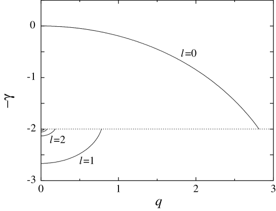
Figure 1: Eigenvalues $-\gamma$ of Eq. (29) versus the wavenumber $q=q_{x}$ for $q_{y}=0$ and $c=1$.

III.1 The case $0<p_{0}n_{r}<\frac{n}{2}$

In this case, we have that $c>0$ in both the diffusion and reaction sectors.

After the relaxation time, the dynamics is dominated by the first Fourier components $X_{0}$, $X_{+1}$, and $X_{-1}$:

$$X\simeq X_{0}+X_{+1}\;{\rm e}^{+i\varphi}+X_{-1}\;{\rm e}^{-i\varphi}\;.$$ (31)

In view of the latter relation, we introduce the densities

$$\rho_{+} \equiv \rho_{A}+\rho_{B}=\int_{-\pi}^{+\pi}f(\vec{r},\varphi)\;d\varphi=2\pi f_{0}\;,$$ (32)

$$\rho_{-} \equiv \rho_{A}-\rho_{B}=\int_{-\pi}^{+\pi}g(\vec{r},\varphi)\;d\varphi=2\pi g_{0}\;.$$ (33)

Thus the zeroth-order expansion of the distribution function $f$ can be related to the total density. Similarly, we introduce the currents

$$\vec{J}_{+} \equiv \vec{J}_{A}+\vec{J}_{B}=\int_{-\pi}^{+\pi}\vec{v}\;f(\vec{r},\varphi)\;d\varphi\;,$$ (34)

$$\vec{J}_{-} \equiv \vec{J}_{A}-\vec{J}_{B}=\int_{-\pi}^{+\pi}\vec{v}\;g(\vec{r},\varphi)\;d\varphi\;.$$ (35)

The first-order Fourier components $X_{+1}$ and $X_{-1}$ are related to the current. As a consequence, we obtain the distribution functions $f$ and $g$ in terms of the corresponding densities and currents

$$f \simeq \frac{1}{2\pi}\left(\rho_{+}+\frac{2}{v^{2}}\vec{v}\cdot\vec{J}_{+}\right)\;,$$ (36)

$$g \simeq \frac{1}{2\pi}\left(\rho_{-}+\frac{2}{v^{2}}\vec{v}\cdot\vec{J}_{-}\right)\;.$$ (37)

The distribution functions for the species $A$ and $B$ are thus given by

$$f_{A} \simeq \frac{1}{2\pi}\left(\rho_{A}+\frac{2}{v^{2}}\vec{v}\cdot\vec{J}_{A}\right)\;,$$ (38)

$$f_{B} \simeq \frac{1}{2\pi}\left(\rho_{B}+\frac{2}{v^{2}}\vec{v}\cdot\vec{J}_{B}\right)\;.$$ (39)

Equations (25) for $l=0$ and $l=\pm 1$ then lead to the coupled equations:

$$\partial_{t}\rho_{+} = -\vec{\nabla}\cdot\vec{J}_{+}\;,$$ (40)

$$\partial_{t}\vec{J}_{+} = -\frac{8av}{3}n\vec{J}_{+}-\frac{v^{2}}{2}\vec{\nabla}\rho_{+}\;,$$ (41)

and

$$\partial_{t}\rho_{-} = -\vec{\nabla}\cdot\vec{J}_{-}-4avp_{0}n_{r}\rho_{-}\;,$$ (42)

$$\partial_{t}\vec{J}_{-} = -\frac{8av}{3}\left(n-\frac{p_{0}n_{r}}{2}\right)\vec{J}_{-}-\frac{v^{2}}{2}\vec{\nabla}\rho_{-}\;.$$ (43)

We notice that the currents relax on a fast time scale so that we can assume that they quickly adjust to their value in a quasi-stationary state as

$$\vec{J}_{+} = -D\vec{\nabla}\rho_{+}\;,\qquad\mbox{for}\quad t\gg\frac{3}{8avn}\;,$$ (44)

$$\vec{J}_{-} = -D^{\rm(r)}\vec{\nabla}\rho_{-}\;,\qquad\mbox{for}\quad t\gg\frac{3}{8av\left(n-\frac{p_{0}n_{r}}{2}\right)}\;,$$ (45)

with the diffusion coefficient

$$D=\frac{3v}{16an}\;,$$ (46)

and the reactive diffusion coefficient

$$D^{\rm(r)}=\frac{3v}{16a\left(n-\frac{p_{0}n_{r}}{2}\right)}\;.$$ (47)

Equation (44) is the expression of Fick’s law for the particles while Eq. (45) is its reactive analogue. Substituting Eqs. (44) and (45) into Eqs. (40) and (42) for the densities, we obtain the diffusion equation

$$\partial_{t}\rho_{+}=D\nabla^{2}\rho_{+}\;,$$ (48)

as well as the reaction-diffusion equation

$$\partial_{t}\rho_{-}=D^{\rm(r)}\nabla^{2}\rho_{-}-2\kappa\rho_{-}\;,$$ (49)

with the reaction rate constant

$$\kappa=2avp_{0}n_{r}\;.$$ (50)

This result shows that the reaction rate constant is the product of the speed $v$ with the cross section $2a$ of the disks, multiplied by the density $n_{r}$ of the catalytic scatterers and weighted by the probability of reaction $p_{0}$. The two equations (48) and (49) show the existence of two slow modes in the system corresponding to the decay rate (30) with $l=0$, namely, the diffusive mode of dispersion relation

$$\mbox{diffusive mode:}\qquad\Gamma=Dq^{2}+O(q^{4})\;,$$ (51)

and the reactive mode of dispersion relation

$$\mbox{reactive mode:}\qquad\Gamma=2\kappa+D^{\rm(r)}q^{2}+O(q^{4})\;.$$ (52)

The equations of motion (48) and (49) determines the time evolution of the densities $\rho_{A}=(\rho_{+}+\rho_{-})/2$ and $\rho_{B}=(\rho_{+}-\rho_{-})/2$ according to the coupled reaction-diffusion equations:

$$\partial_{t}\rho_{A} = D_{AA}\nabla^{2}\rho_{A}+D_{AB}\nabla^{2}\rho_{B}-\kappa(\rho_{A}-\rho_{B})\;,$$ (53)

$$\partial_{t}\rho_{B} = D_{BA}\nabla^{2}\rho_{A}+D_{BB}\nabla^{2}\rho_{B}+\kappa(\rho_{A}-\rho_{B})\;,$$ (54)

where the transport coefficients can be identified as

$$D_{AA} = D_{BB}=\frac{D+D^{\rm(r)}}{2}\;,$$ (55)

$$D_{AB} = D_{BA}=\frac{D-D^{\rm(r)}}{2}\;.$$ (56)

The important conclusion is here that there appears a phenomenon of cross diffusion which is induced by the reaction. Indeed, the cross-diffusion coefficient takes the value

$$D_{AB}=D_{BA}=-\frac{3vp_{0}n_{r}}{64an\left(n-\frac{p_{0}n_{r}}{2}\right)}\;,$$ (57)

which vanishes with the reaction probability $p_{0}$ and the density of catalysts $n_{r}$. In the absence of reaction, the cross-diffusion terms vanish with the reaction term and we recover two uncoupled diffusion equations for $A$ and $B$ particles.

We notice that the coupled reaction-diffusion equations (53)-(54) can be rewritten as

$$\partial_{t}\rho_{A} = -\vec{\nabla}\cdot\vec{J}_{A}-\kappa(\rho_{A}-\rho_{B})\;,$$ (58)

$$\partial_{t}\rho_{B} = -\vec{\nabla}\cdot\vec{J}_{B}+\kappa(\rho_{A}-\rho_{B})\;,$$ (59)

in terms of the currents:

$$\vec{J}_{A} = -\frac{D+D^{\rm(r)}}{2}\vec{\nabla}\rho_{A}-\frac{D-D^{\rm(r)}}{2}\vec{\nabla}\rho_{B}\;,$$ (60)

$$\vec{J}_{B} = -\frac{D+D^{\rm(r)}}{2}\vec{\nabla}\rho_{B}-\frac{D-D^{\rm(r)}}{2}\vec{\nabla}\rho_{A}\;.$$ (61)

Besides the diffusive and reactive slowest modes, we also find faster modes often referred to as kinetic modes. All these modes exist in both the diffusion sector ruled by Eq. (23) for $X=f$ and in the reaction sector ruled by Eq. (23) for $X=h$. All these modes are characterized by dispersion relations which form a whole spectrum. Figure 2 depicts the whole spectra of the diffusionand reaction sectors in the case $0<p_{0}n_{r}<\frac{n}{2}$.

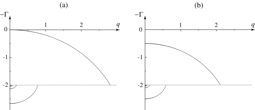
Figure 2: Eigenvalues $-\Gamma$ versus the wavenumber $q=q_{x}$ for $q_{y}=0$ in the regime $0<p_{0}n_{r}<\frac{n}{2}$ where $c>0$: (a) spectrum of the diffusion sector; (b) spectrum of the reaction sector. The parameter values are $av=1$, $n=1$, and $p_{0}n_{r}=0.125$.

III.2 The case $p_{0}n_{r}=\frac{n}{2}$

In this case, we remark that Eq. (23) for $X=h$ has a vanishing coefficient $c=0$ in the reaction sector so that the equation for $X=h$ is purely advective

$$\partial_{t}h+\vec{v}\cdot\vec{\nabla}h=0\;.$$ (62)

Its solutions are given by $h=h(\vec{r}-\vec{v}t)$ and $g={\rm e}^{-2\kappa t}h(\vec{r}-\vec{v}t)$ obeys

$$\partial_{t}g+\vec{v}\cdot\vec{\nabla}g=-2\kappa g\;.$$ (63)

In this case, there is no reactive diffusion coefficient which characterizes the reactive process.

III.3 The case $\frac{n}{2}<p_{0}n_{r}<n$

As we noticed before, $p_{0}n_{r}$ cannot exceed the value $n$ for consistency. In this case, we have that Eq. (23) for $X=f$ still has a coefficient $c>0$ in the diffusion sector but Eq. (23) for $X=h$ has a negative coefficient $c<0$ in the reaction sector. Accordingly, the spectrum shown in Fig. 1 is upside down in the reaction sector and the slowest reactive mode is no longer the same as before.

Here, we must consider the decay rate (30) with $l=1$. The dispersion relation of the reactive mode is now given by

$$\Gamma=2\kappa^{\prime}+{D^{\rm(r)}}^{\prime}q^{2}\;,$$ (64)

with the new reaction constant

$$\kappa^{\prime}=\frac{2av}{3}(2n-p_{0}n_{r})\;,$$ (65)

and the new reactive diffusion coefficient

$${D^{\rm(r)}}^{\prime}=\frac{9v}{16a(2p_{0}n_{r}-n)}\;.$$ (66)

A transition should therefore appear at high concentrations of catalysts.

Figure 3 depicts the spectra in the diffusion and reaction sectors in the case $\frac{n}{2}<p_{0}n_{r}<n$.

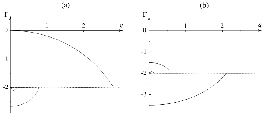
Figure 3: Eigenvalues $-\Gamma$ versus the wavenumber $q=q_{x}$ for $q_{y}=0$ in the regime $\frac{n}{2}<p_{0}n_{r}<n$ where $c>0$: (a) spectrum of the diffusion sector; (b) spectrum of the reaction sector. The parameter values are $av=1$, $n=1$, and $p_{0}n_{r}=0.875$.

In the following, we shall focus on the case $0<p_{0}n_{r}<\frac{n}{2}$ where the catalysts are dilute enough.

IV The entropy balance

In this section, we derive the equation for the balance of entropy from the $H$-theorem in two approximations for the entropy density. In kinetic theory, we have a well-defined expression for the entropy which guarantees that the entropy production is always non-negative. However, at the level of the macroscopic description given by the reaction-diffusion equations (53)-(54), the entropy is given as an approximation of the expression (12) of kinetic theory and we must verify the domain of validity where the corresponding entropy production is non-negative.

The first approximation we consider is based on the standard phenomenological entropy defined in irreversible thermodynamics of reaction processes dGM ; KoPr98 . We show that the corresponding entropy production is non-negative in a broad range of values for the densities $\rho_{A}$ and $\rho_{B}$ including the thermodynamic equilibrium state but there is a small domain where the entropy production corresponding to this approximation fails to remain non-negative.

Therefore, we consider a second approximation which includes extra terms involving the gradient of the densities. We show that the corresponding entropy production always remains non-negative.

IV.1 Entropy without gradients

Supposing that the system is sufficiently dilute, the phenomenological irreversible thermodynamics supposes that the entropy density has the following expression:

$$s=\rho_{A}\ln\frac{\rho^{0}}{\rho_{A}}+\rho_{B}\ln\frac{\rho^{0}}{\rho_{B}}\;.$$ (67)

This entropy density is obtained from the entropy (12) of kinetic theory by using the expansions (38) and (39) of the distribution functions and by keeping the terms in the densities themselves and discarding terms in the gradients. The reference density is thus given by $\rho^{0}=2\pi f^{0}$, which amounts to suppose the equality of the masses of the particles $A$ and $B$.

The variation of the entropy density $s$ in time is given by

$$\partial_{t}s=-\vec{\nabla}\cdot\vec{J}_{s}+\sigma_{s}\;,$$ (68)

as calculated by using the coupled reaction-diffusion equations (58)-(59). The entropy current density is obtained in terms of the currents (60) and (61) of particles $A$ and $B$ as

$$\vec{J}_{s}=\vec{J}_{A}\ln\frac{\rho^{0}}{{\rm e}\rho_{A}}+\vec{J}_{B}\ln\frac{\rho^{0}}{{\rm e}\rho_{B}}\;,$$ (69)

while the entropy production as

$$\sigma_{s}=\kappa(\rho_{A}-\rho_{B})\ln\frac{\rho_{A}}{\rho_{B}}-\vec{J}_{A}\cdot\frac{\vec{\nabla}\rho_{A}}{\rho_{A}}-\vec{J}_{B}\cdot\frac{\vec{\nabla}\rho_{B}}{\rho_{B}}\;.$$ (70)

Inverting Eqs. (60) and (61), we obtain the gradients in terms of the currents as

$$\vec{\nabla}\rho_{A} = -\frac{\vec{J}_{A}}{D}+\frac{2\kappa}{3v^{2}}(\vec{J}_{A}-\vec{J}_{B})\;,$$ (71)

$$\vec{\nabla}\rho_{B} = -\frac{\vec{J}_{B}}{D}-\frac{2\kappa}{3v^{2}}(\vec{J}_{A}-\vec{J}_{B})\;.$$ (72)

Substituting in the entropy production (70), we get

$$\sigma_{s}=\kappa(\rho_{A}-\rho_{B})\ln\frac{\rho_{A}}{\rho_{B}}+\alpha\vec{J}_{A}^{2}+2\beta\vec{J}_{A}\cdot\vec{J}_{B}+\gamma\vec{J}_{B}^{2}\;,$$ (73)

with the coefficients

$$\alpha = \frac{1}{\rho_{A}}\left(\frac{1}{D}-\frac{2\kappa}{3v^{2}}\right)\;,$$ (74)

$$\beta = \frac{\kappa}{3v^{2}}\left(\frac{1}{\rho_{A}}+\frac{1}{\rho_{B}}\right)\;,$$ (75)

$$\gamma = \frac{1}{\rho_{B}}\left(\frac{1}{D}-\frac{2\kappa}{3v^{2}}\right)\;.$$ (76)

The first term in the entropy production (73) is always non-negative because $(x-y)\ln(x/y)\geq 0$ for all positive values of the real numbers $x$ and $y$. On the other hand, the last terms constitute a quadratic form which is non-negative under the conditions that $\beta^{2}-\alpha\gamma<0$ with $\alpha>0$ and $\gamma>0$. For the diffusion coefficient (46), we check that

$$\alpha = \frac{4a}{3v\rho_{A}}(4n-p_{0}n_{r})>0\;,$$ (77)

$$\gamma = \frac{4a}{3v\rho_{B}}(4n-p_{0}n_{r})>0\;,$$ (78)

because of the consistency condition (22). Next, the condition $\beta^{2}-\alpha\gamma<0$ is given by

$$\xi^{2}+2\left[1-2\left(\frac{2}{y}-1\right)^{2}\right]\,\xi+1<0\;,$$ (79)

in terms of the density ratio

$$\xi\equiv\frac{\rho_{B}}{\rho_{A}}\;,$$ (80)

and the parameter

$$y\equiv\frac{p_{0}n_{r}}{2n}=\frac{4\kappa D}{3v^{2}}\;.$$ (81)

The roots $\xi_{\pm}$ of Eq. (79) satisfy $\xi_{+}=\frac{1}{\xi_{-}}$. If $\xi_{+}\geq\xi_{-}$, the entropy production is thus non-negative in the domain

$$\xi_{+}\rho_{A}\geq\rho_{B}\geq\xi_{-}\rho_{A}\;.$$ (82)

It turns out that the sum of the roots

$$\xi_{+}+\xi_{-}=2\left[2\left(\frac{2}{y}-1\right)^{2}-1\right]\;,$$ (83)

is always positive in the interval $0<y<\frac{1}{2}$ where the condition of consistency (22) is verified. (The sum $\xi_{+}+\xi_{-}$ is negative only in the interval $4-2\sqrt{2}=1.1715...<y<4+2\sqrt{2}=6.8284...$ outside the domain of consistency.) Since $\xi_{+}$ and $\xi_{-}$ have the same sign, they both are positive in the consistency domain $0<y<\frac{1}{2}$, which means that there exists a domain of the quadrant ($\rho_{A}\geq 0$, $\rho_{B}\geq 0$) where the entropy production (73) can be negative. This domain is composed of $\xi_{-}\;\rho_{A}>\rho_{B}\geq 0$ and $\xi_{-}\;\rho_{B}>\rho_{A}\geq 0$. Another way of saying it is that the domain (82) where the entropy production is non-negativity is smaller than the quadrant ($\rho_{A}\geq 0$, $\rho_{B}\geq 0$) of all the possible densities $\rho_{A}$ and $\rho_{B}$. The domain of non-negativity extends to

$$1441.9...\,\rho_{A}\geq\rho_{B}\geq 0.00069348...\,\rho_{A}\;,\qquad\mbox{for}\quad y=0.1\;,$$ (84)

to

$$321.99...\,\rho_{A}\geq\rho_{B}\geq 0.0031056...\,\rho_{A}\;,\qquad\mbox{for}\quad y=0.2\;,$$ (85)

and to

$$33.970...\,\rho_{A}\geq\rho_{B}\geq 0.029437...\,\rho_{A}\;,\qquad\mbox{for}\quad y=0.5\;.$$ (86)

It is only in the limit $y=0$ without chemical reaction that the domain of non-negativity coincides with the quadrant ($\rho_{A}\geq 0$, $\rho_{B}\geq 0$). In the presence of the chemical reaction, the situation is unsatisfactory because the scheme is not consistent with the second law of thermodynamics even if the domain of negative entropy production is small and only concerns color densities which are very far from the thermodynamic equilibrium.

IV.2 Entropy with gradients

To cure the problem reported here above, we choose to expand the entropy production (12) of kinetic theory to include the terms with gradients of the densities. For this purpose, we substitute the expansions (38) and (39) of the distribution functions in the entropy (12) and we truncate up to the terms which are quadratic in the currents to get

$$s=\rho_{A}\ln\frac{\rho^{0}}{\rho_{A}}+\rho_{B}\ln\frac{\rho^{0}}{\rho_{B}}-\frac{1}{v^{2}}\left(\frac{\vec{J}_{A}^{2}}{\rho_{A}}+\frac{\vec{J}_{B}^{2}}{\rho_{B}}\right)\;,$$ (87)

where the particle currents are given in terms of the density gradients according to Eqs. (60) and (61). Accordingly, the entropy (87) is quadratic in the density gradients.

Here again, we calculate the time variation of the entropy density $s$ by using the coupled reaction-diffusion equations (58)-(59). The balance equation for entropy is here also given by

$$\partial_{t}s=-\vec{\nabla}\cdot\vec{J}_{s}+\sigma_{s}\;,$$ (88)

with an entropy current similar to Eq. (69)

$$\vec{J}_{s}=\vec{J}_{A}\ln\frac{\rho^{0}}{{\rm e}\rho_{A}}+\vec{J}_{B}\ln\frac{\rho^{0}}{{\rm e}\rho_{B}}+O(3)\;,$$ (89)

up to the terms $O(3)$ of third order in the gradients. However, the entropy production now takes the more complicated form

$$\sigma_{s}=\kappa(\rho_{A}-\rho_{B})\ln\frac{\rho_{A}}{\rho_{B}}-\vec{J}_{A}\cdot\frac{\vec{\nabla}\rho_{A}}{\rho_{A}}-\vec{J}_{B}\cdot\frac{\vec{\nabla}\rho_{B}}{\rho_{B}}+\frac{2\kappa}{v^{2}}(\vec{J}_{A}-\vec{J}_{B})\cdot\left(\frac{\vec{J}_{A}}{\rho_{A}}-\frac{\vec{J}_{B}}{\rho_{B}}\right)-\frac{\kappa}{v^{2}}(\rho_{A}-\rho_{B})\left(\frac{\vec{J}_{A}^{2}}{\rho_{A}^{2}}-\frac{\vec{J}_{B}^{2}}{\rho_{B}^{2}}\right)+O(4)\;,$$ (90)

where $O(4)$ denotes terms of fourth order in the gradients. Replacing the gradients by the currents with Eqs. (71)-(72), we obtain

$$\sigma_{s}=\kappa(\rho_{A}-\rho_{B})\ln\frac{\rho_{A}}{\rho_{B}}+\frac{1}{D}\left(\frac{\vec{J}_{A}^{2}}{\rho_{A}}+\frac{\vec{J}_{B}^{2}}{\rho_{B}}\right)+\frac{4\kappa}{3v^{2}}(\vec{J}_{A}-\vec{J}_{B})\cdot\left(\frac{\vec{J}_{A}}{\rho_{A}}-\frac{\vec{J}_{B}}{\rho_{B}}\right)-\frac{\kappa}{v^{2}}(\rho_{A}-\rho_{B})\left(\frac{\vec{J}_{A}^{2}}{\rho_{A}^{2}}-\frac{\vec{J}_{B}^{2}}{\rho_{B}^{2}}\right)+O(4)\;,$$ (91)

or equivalently

$$\sigma_{s}=\kappa(\rho_{A}-\rho_{B})\ln\frac{\rho_{A}}{\rho_{B}}+\alpha\vec{J}_{A}^{2}+2\beta\vec{J}_{A}\cdot\vec{J}_{B}+\gamma\vec{J}_{B}^{2}+O(4)\;,$$ (92)

with the coefficients

$$\alpha = \frac{1}{\rho_{A}}\left(\frac{1}{D}+\frac{\kappa}{3v^{2}}+\frac{\kappa\rho_{B}}{v^{2}\rho_{A}}\right)\;,$$ (93)

$$\beta = -\frac{2\kappa}{3v^{2}}\left(\frac{1}{\rho_{A}}+\frac{1}{\rho_{B}}\right)\;,$$ (94)

$$\gamma = \frac{1}{\rho_{B}}\left(\frac{1}{D}+\frac{\kappa}{3v^{2}}+\frac{\kappa\rho_{A}}{v^{2}\rho_{B}}\right)\;.$$ (95)

The coefficients $\alpha$ and $\gamma$ are always positive, while the condition $\beta^{2}-\alpha\gamma<0$ of non-negativity of the quadratic form is here given by

$$\xi^{2}+2\frac{(y+2)^{2}+4}{y(12-y)}\,\xi+1>0\;,$$ (96)

with the ratio $\xi$ defined by Eq. (80) and the parameter $0<y<\frac{1}{2}$ by Eq. (81). The opposite inequality is obtained compared to Eq. (79) because the dependence on the ratio $\xi$ is here more complicated but still simple enough to lead to the quadratic equation (96). In the physical domain $0<y<\frac{1}{2}$, the roots $\xi_{+}$ and $\xi_{-}=1/\xi_{+}$ of Eq. (96) are real and negative because

$$\xi_{+}+\xi_{-}=-2\frac{(y+2)^{2}+4}{y(12-y)}<0\;.$$ (97)

As a consequence, the quadratic part of the entropy production (92) is non-negative in the quadrant of all the physically allowed densities where $\rho_{A}\geq 0$ and $\rho_{B}\geq 0$. If the gradients of densities are small enough so that the corrections of fourth order in Eq. (92) are negligible, the whole entropy production (92) is also non-negative.

We have thus proved that the inclusion of the gradient terms in the entropy avoids the aforementioned problem and guarantees that the entropy production remains non-negative for all the values of the color densities if the gradients are sufficiently small.

IV.3 Interpretation of the gradient terms in the entropy

The entropy density given by Eq. (87) can be expressed as follows in terms of the gradients of the particle densities by using Eqs. (60)-(61)

$$s=\rho_{A}\ln\frac{\rho^{0}}{\rho_{A}}+\rho_{B}\ln\frac{\rho^{0}}{\rho_{B}}-\frac{K_{AA}}{2}\left(\vec{\nabla}\rho_{A}\right)^{2}-K_{AB}\vec{\nabla}\rho_{A}\cdot\vec{\nabla}\rho_{B}-\frac{K_{BB}}{2}\left(\vec{\nabla}\rho_{B}\right)^{2}\;,$$ (98)

with the coefficients

$$K_{AA} = \frac{\left(D+D^{\rm(r)}\right)^{2}}{2v^{2}\rho_{A}}+\frac{\left(D-D^{\rm(r)}\right)^{2}}{2v^{2}\rho_{B}}\;,$$ (99)

$$K_{BB} = \frac{\left(D+D^{\rm(r)}\right)^{2}}{2v^{2}\rho_{B}}+\frac{\left(D-D^{\rm(r)}\right)^{2}}{2v^{2}\rho_{A}}\;,$$ (100)

$$K_{AB} = \frac{\left(D+D^{\rm(r)}\right)\left(D-D^{\rm(r)}\right)}{2v^{2}}\left(\frac{1}{\rho_{A}}+\frac{1}{\rho_{B}}\right)\;,$$ (101)

which are independent of the velocity $v$.

The gradient terms are of the same kind as those appearing in the Ginzburg-Landau free energy. Here, they appear in the entropy with the opposite sign in agreement with the required thermodynamic stability of the equilibrium state PeFi90 ; WaSeWh93 . Indeed, the entropy must be maximal in a stable equilibrium state which is the case since the quadratic form in Eq. (87) or (98) is negative. Accordingly, the entropy reaches a maximum at the equilibrium state where the gradients and the currents vanish.

The gradient terms are responsible for statistical correlations between the particles. Indeed, the entropy density (98) can be used to define the entropy functional

$$S[\rho_{A},\rho_{B}]=\int s\;d\vec{r}\;,$$ (102)

and the probability distribution for statistical average given by the functional integrals

$$\langle{\cal O}\rangle_{\rm eq}=\frac{\int{\cal D}\rho_{A}{\cal D}\rho_{B}\;{\cal O}\;\exp\left(\frac{1}{k_{\rm B}}S[\rho_{A},\rho_{B}]\right)}{\int{\cal D}\rho_{A}{\cal D}\rho_{B}\;\exp\left(\frac{1}{k_{\rm B}}S[\rho_{A},\rho_{B}]\right)}\;,$$ (103)

for an observable $\cal O$. This allows us to calculate the correlation functions of the particle densities at the thermodynamic equilibrium. We consider the correlation functions of the densities (32)-(33):

$$C_{++}(\vec{r}) \equiv \langle\rho_{+}(\vec{r})\rho_{+}(0)\rangle_{\rm eq}-\langle\rho_{+}\rangle_{\rm eq}^{2}\;,$$ (104)

$$C_{--}(\vec{r}) \equiv \langle\rho_{-}(\vec{r})\rho_{-}(0)\rangle_{\rm eq}-\langle\rho_{-}\rangle_{\rm eq}^{2}\;,$$ (105)

$$C_{+-}(\vec{r}) \equiv \langle\rho_{+}(\vec{r})\rho_{-}(0)\rangle_{\rm eq}-\langle\rho_{+}\rangle_{\rm eq}\,\langle\rho_{-}\rangle_{\rm eq}\;.$$ (106)

Partial differential equations can be obtained for these correlation functions by the variational principle $\delta S=0$ based on the entropy functional (98) evaluated around the thermodynamic equilibrium

$$s\simeq s_{\rm eq}-\frac{(\rho_{+}-\rho_{\rm eq})^{2}+\rho_{-}^{2}}{2\,\rho_{\rm eq}}-\frac{K_{++,{\rm eq}}}{2}\left(\vec{\nabla}\rho_{+}\right)^{2}-\frac{K_{--,{\rm eq}}}{2}\left(\vec{\nabla}\rho_{-}\right)^{2}\;,$$ (107)

where the equilibrium values of the coefficients are given by $\langle\rho_{+}\rangle_{\rm eq}=\rho_{\rm eq}=\frac{2}{\rm e}\rho^{0}$, $\langle\rho_{-}\rangle_{\rm eq}=0$, $s_{\rm eq}=\rho_{\rm eq}$, and

$$K_{++,{\rm eq}} = \frac{1}{4}\left(K_{AA}+K_{BB}+2K_{AB}\right)_{\rm eq}=\frac{2D^{2}}{v^{2}\rho_{\rm eq}}\;,$$ (108)

$$K_{--,{\rm eq}} = \frac{1}{4}\left(K_{AA}+K_{BB}-2K_{AB}\right)_{\rm eq}=\frac{2D^{\rm(r)\,2}}{v^{2}\rho_{\rm eq}}\;,$$ (109)

$$K_{+-,{\rm eq}} = \frac{1}{4}\left(K_{AA}-K_{BB}\right)_{\rm eq}=0\;,$$ (110)

so that there is no cross term in the gradients of $\rho_{\pm}$ in Eq. (107). The fluctuations described by Eq. (103) are Gaussian around the equilibrium since the entropy density (107) is quadratic. As a consequence, the correlation functions obey the equations

$$\left(\nabla^{2}-\frac{1}{\ell_{+}^{2}}\right)C_{++}(\vec{r})=0\;,$$ (111)

$$\left(\nabla^{2}-\frac{1}{\ell_{-}^{2}}\right)C_{--}(\vec{r})=0\;,$$ (112)

for $\vec{r}\neq 0$ and with the correlation lengths

$$\ell_{+} \equiv \sqrt{\rho_{\rm eq}K_{++,{\rm eq}}}=\frac{3\sqrt{2}}{16an}\;,$$ (113)

$$\ell_{-} \equiv \sqrt{\rho_{\rm eq}K_{--,{\rm eq}}}=\frac{3\sqrt{2}}{16a\left(n-\frac{p_{0}n_{r}}{2}\right)}\;,$$ (114)

and $C_{+-}(\vec{r})=0$. These correlation lengths are of the order of the mean free path of the particles between the scatterers of radius $a$ and density $n$. The correlation functions are given by Bessel functions of zeroth order and they behave at long distance as

$$C_{\pm\pm}(\vec{r})\sim\frac{1}{\sqrt{r}}\;\exp\left(-\frac{r}{\ell_{\pm}}\right)\;,$$ (115)

with $r=\sqrt{\vec{r}^{\,2}}$.

V Conclusions

In this paper, we have studied a reactive random Lorentz gas in which a point particle carrying a color $A$ or $B$ (or a spin one-half) bounces among randomly distributed disk scatterers. Some of these disks are catalytic in the sense that the reaction $A\rightleftharpoons B$ occurs with a given probability $p_{0}$ upon collision on these catalytic disks. In the case of a particle with a spin, the catalytic disks correspond to impurities flipping the spin. Under dilute-gas conditions, the time evolution of the distribution functions of finding the particle with a given color or spin at some position $\vec{r}$ with some velocity $\vec{v}$ are ruled by two coupled Boltzmann-Lorentz kinetic equations which satisfy a $H$-theorem. The $H$-quantity defines the entropy at the kinetic level of description.

The time evolution separates into a diffusion sector for the total distribution function and a reaction sector for the difference of the distribution functions of the colors. The spectrum of eigenmodes of both sectors can be constructed in detail. The diffusive (resp. reactive) modes are the slowest modes among all the modes of the diffusion (resp. reaction) sector, which provides us with the diffusion coefficient of the diffusive mode, as well as the reaction rate constant and the reactive diffusion coefficient of the reactive mode. This analysis and the knowledge of these coefficients allow us to obtain the macroscopic reaction-diffusion equations. These equations present cross-diffusion terms which are induced by the reaction if the reaction probability $p_{0}$ is not vanishing, as in the previous studies of the reactive periodic Lorentz gas and multibaker models GaKl98 ; Ga99 ; ClGa00 ; ClGa02 ; GaCl02 . In the reactive random Lorentz gas, our analysis shows that a transition happens in the reaction sector between a regime at low concentrations of catalytic disks and reaction probabilities and another one at high concentrations and probabilities.

Using the derivation of the macroscopic reaction-diffusion equations, we have studied the problem of the entropy production on the basis of the entropy defined in kinetic theory in terms of the distribution functions and the associated $H$-theorem. The entropy of kinetic theory can be expanded in powers of the gradients of the densities of both colors $A$ and $B$. At the lowest order of this expansion, the entropy density is simply a function of the color densities themselves and coincides with the expression of the phenomenological nonequilibrium thermodynamics dGM ; KoPr98 . The balance equation of this entropy without gradient can be derived from the macroscopic reaction-diffusion equations. Because of the cross-diffusion effects induced by the reaction, the resulting entropy production may become negative for extreme values of the ratio between the color densities. This is certainly a problem of principle for the phenomenological approach. In order to solve this problem, we have considered the entropy density at the next order of the expansion in the gradients of color densities. At this next order, the entropy density contains terms which are quadratic in the gradients beside the contribution of the phenomenological entropy. The balance equation of this entropy with gradients turns out to have an entropy production which is non-negative for all the color densities and for small enough gradients of color densities, in consistency with the second law of thermodynamics.

The entropy density with gradients is interpreted as the entropic version of the Ginzburg-Landau free energy. The addition of gradient terms are shown to be responsible for statistical correlations in the densities of the colors $A$ and $B$ over spatial scales of the order of the mean free path of the particle. The consideration of these spatial correlations appears to be necessary to get a non-negative entropy production in the presence of chemically induced cross diffusion. The inclusion of these gradients in the entropy is justified by the kinetic theory and by the consistency so obtained with the second law of thermodynamics. Such an entropy functional with gradients is also justifed by analogy with the Ginzburg-Landau free energy PeFi90 ; WaSeWh93 . The inclusion of gradients in the entropy requires a departure from the classical Onsager-Prigogine nonequilibrium thermodynamics dGM ; KoPr98 . This classical nonequilibrium thermodynamics neglects the possible interplay between the diffusion and the reaction, such as the cross diffusion induced by the chemical reaction. This effect is expected in systems with a high reaction probability and high concentrations of reactants with respect to the inerts species which do not participate to the reaction. We think that the present workk clearly shows that this chemically induced cross diffusion is compatible with kinetic theory and the second law of thermodynamics and should be an experimentally observable effect.

Acknowledgments. The authors thank Professor G. Nicolis for support and encouragement in this research. L.M. is supported through a European Community Marie Curie Fellowship – contract No. HPMF-CT-2002-01511. This research is financially supported by the “Communauté française de Belgique” (“Actions de Recherche Concertées”, contract No. 04/09-312), the National Fund for Scientific Research (F. N. R. S. Belgium), the F. R. F. C. (contract No. 2.4577.04.), and the U.L.B..

References

- (1) D.J. Evans and G.P. Morriss, Statistical Mechanics of Nonequilibrium Liquids (Academic Press, London, 1990);
- (2) P. Gaspard and G. Nicolis, Phys. Rev. Lett. 65, 1693 (1990).
- (3) P. Gaspard, J. Stat. Phys., 68, 673 (1992).
- (4) N.I. Chernov, G.L. Eyink, J.L. Lebowitz, and Ya.G. Sinai, Phys. Rev. Lett. 70, 2209 (1993); Comm. Math. Phys. 154, 569 (1993).
- (5) D. Ruelle, J. Stat. Phys. 85, 1 (1996); 86, 935 (1997).
- (6) P. Gaspard, Chaos, Scattering and Statistical Mechanics, (Cambridge University Press, Cambridge, 1998).
- (7) J.R. Dorfman, An Introduction to Chaos in Nonequilibrium Statistical Mechanics, (Cambridge University Press, Cambridge 1999).
- (8) T. Tél, J. Vollmer, and W. Breymann, Phys. Rev. E, 58, 1672 (1998).
- (9) T. Tél and J. Vollmer, Entropy balance, Multibaker Maps, and the Dynamics of the Lorentz gas, in: D. Szász, Editor, Hard Ball Systems and the Lorentz Gas (Springer-Verlag, Berlin, 2000) pp. 367-418.
- (10) L. Mátyás, T. Tél, and J. Vollmer, Phys. Rev. E 62, 349 (2000).
- (11) S. Tasaki and P. Gaspard, J. Stat. Phys. 101, 125 (2000).
- (12) T. Tél, J. Vollmer, and L. Mátyás, Europhys. Lett. 53, 458 (2001).
- (13) T. Gilbert and J.R. Dorfman, J. Stat. Phys. 96, 225 (1999).
- (14) T. Gilbert, J.R. Dorfman, and P. Gaspard, Phys. Rev. Lett. 85, 1606 (2000).
- (15) J.R. Dorfman, P. Gaspard, and T. Gilbert, Phys. Rev. E 85, 026110 (2002).
- (16) P. Gaspard, G. Nicolis, and J.R. Dorfman, Physica A 323, 294 (2003).
- (17) S. Viscardy and P. Gaspard, Phys. Rev. E 68, 041204 (2003).
- (18) S. Viscardy and P. Gaspard, Phys. Rev. E 68, 041205 (2003).
- (19) G. Nicolis and I. Prigogine, Self-organization in nonequilibrium systems (Wiley, New York, 1977).
- (20) P. Gaspard and R. Klages, Chaos 8, 409 (1998).
- (21) P. Gaspard, Physica A 263, 315 (1999).
- (22) Originally the random Lorentz gas was introduced in a work of Lorentz Lobook05 as a model of electric conduction.
- (23) H. A. Lorentz, Proc. Roy. Acad. Amst. 7, 438, 585, 684 (1905).
- (24) I. Claus and P. Gaspard, J. Stat. Phys. 101, 161 (2000).
- (25) I. Claus, and P. Gaspard, Physica D 168-169, 266 (2002).
- (26) P. Gaspard and I. Claus, Phil. Trans. Roy. Soc. Lond. A 360, 303 (2002).
- (27) S. de Groot and P. Mazur, Non-equilibrium thermodynamics (North-Holland, Amsterdam, 1962; reprinted by Dover Publ. Co., New York, 1984).
- (28) D. Kondepudi and I. Prigogine, Modern Thermodynamics (Wiley, New York, 1998).
- (29) H. van Beijeren, Rev. Mod. Phys. 54, 195 (1982).
- (30) C. Boldrighini, L. A. Bunimovich, and Ya.G. Sinai, J. Stat. Phys. 32, 477 (1983).
- (31) O. Penrose and P.C. Fife, Physica D 43, 44 (1990).
- (32) S.-L. Wang, R.F. Sekerka, A.A. Wheeler, B.T. Murray, S.R. Coriell, R.J. Braun, and G.B. McFadden, Physica D 69, 189 (1993).