Weak noise approach to the logistic map

Abstract

Using a nonperturbative weak noise approach we investigate the interference of noise and chaos in simple 1D maps. We replace the noise-driven 1D map by an area-preserving 2D map modelling the Poincare sections of a conserved dynamical system with unbounded energy manifolds. We analyze the properties of the 2D map and draw conclusions concerning the interference of noise on the nonlinear time evolution. We apply this technique to the standard period-doubling sequence in the logistic map. From the 2D area-preserving analogue we, in addition to the usual period-doubling sequence, obtain a series of period doubled cycles which are elliptic in nature. These cycles are spinning off the real axis at parameters values corresponding to the standard period doubling events.

I Introduction

The noise-induced escape from an equilibrium state is a fundamental problem in many areas in science. The classical work goes back to Kramers Kramers (1940) who computed the transition rate from a single potential well; see also the review in Ref. Hänggi et al. (1990). More recently, the understanding and description of nonlinear dynamical systems exhibiting e.g. period-doubling, intermittency, and chaos, have led to a renewed interest in the influence of noise on the behavior of such systems Graham and Tél (1984a, b); Graham et al. (1985); Graham and Tél (1986); Graham (1989); Mos (1989).

In this context the generation of chaotic motion in low dimensional time-discrete systems Collet and Eckmann (1980); Grossmann and Thomae (1977); Feigenbaum (1978, 1979) offers a particularly simple case lending itself to the analysis of the influence of noise. Thus a variety of phenomena have been investigated such as the noise-induced shift, broadening, and suppression of bifurcations Haken and Mayer-Kress (1981); Linz and Lücke (1986), the scaling properties of Lyapunov exponents Crutchfield et al. (1981); Shraiman et al. (1981) and the invariant density Reimann and Talkner (1991a); Graham et al. (1991) near the threshold for chaos, the scaling of intermittency Hirsch et al. (1982), and escape from locally stable states Arecchi et al. (1984); Grassberger (1989); Talkner et al. ; Crutchfield et al. (1982); Reimann and Talkner (1991a, b); Reimann et al. (1994); Reimann and Talkner (1995); see also recent work on the application of periodic orbit theory to noisy maps Cvitanovic et al. (1998); Cvitanovic et al. (1999a, b).

For the purpose of studying the interference of stochastic noise with the nonlinear behavior of dynamical systems, the simplest case is the influence of noise on 1-D maps of the generic type

$$x_{n+1}=f(x_{n}).$$ (1)

Here $n$ is the discrete time index and the map $f(x)$ defines the nonlinear discrete time evolution. In the linear case $f(x)\propto x$ the map is readily analyzed; it possesses an attractive or repulsive fixed point at $x=0$ depending on the slope, and does not exhibit chaos. In the nonlinear case, where $f(x)$ possesses one or several differentiable maxima, the map generates the well-known period-doubling sequence to a chaotic state beyond a critical value of the control parameter characterizing the map Feigenbaum (1978, 1979). In the singular case of for example the tent or the shift map, the period-doubling sequence is absent and the time evolution becomes chaotic beyond a critical control parameter value, see e.g. Refs. Ott (1993); Schuster (1989); Strogatz (1994) .

Assuming that the deterministic map in Eq. (1) describes the dynamical evolution of a nonlinear system in an effectively reduced phase space, the presence of stochastic degrees of freedom originating from the environment can typically be modelled by an additive noise term and we are led to the stochastic map

$$x_{n+1}=f(x_{n})+\xi_{n};$$ (2)

a discrete version of the usual Langevin equation for stochastic processes van Kampen (1992).

Here $\xi_{n}$ indicates the applied noise which we for simplicity assume has a Gaussian distribution

$$P(\xi_{n})=\frac{1}{\sqrt{2\pi\Delta}}\exp\left[-\frac{\xi_{n}^{2}}{2\Delta}\right],$$ (3)

and is correlated according to

$$\langle\xi_{n}\xi_{m}\rangle=\Delta\delta_{nm},$$ (4)

where $\Delta$ is the noise strength and $\langle\cdots\rangle$ indicates an average over the noise ensemble.

The map $f$ acts like a nonlinear filter on the known white noise input fluctuations $\xi_{n}$ and the fundamental issue becomes that of determining the stochastic properties of the stochastic variable $x_{n}$. The natural small parameter is the noise strength $\Delta$ which enters in a nonperturbative manner as indicated by the form of $P(\xi)$ in Eq. (3). Physically, the case of vanishing noise $\Delta=0$, yielding the dissipative map in Eq. (1) for $\xi=0$, is quite distinct from the case of weak noise $\Delta\sim 0$, where on a sufficiently long time scale (labelled by the iteration index n) the noise $\xi_{n}$ drives the variable $x_{n}$ into a stochastic state. The issue is to understand how the stochastic noise interferes with the nonlinear behavior.

In recent work we have elaborated on a nonperturbative canonical phase space approach based on the Freidlin-Wentzel formulation Freidlin and Wentzel (1998) or, alternatively, a saddle point approximation to the Martin-Siggia-Rose method in its functional form Martin et al. (1973); Baussch et al. (1976) and have applied this scheme to the stochastic Kardar-Parisi-Zhang equation Medina et al. (1989); Kardar et al. (1986) describing the evolution of a growing interface Fogedby et al. (1995); Fogedby (1998, 1999); Fogedby and Brandenburg (2002); Fogedby (2003).

It is characteristic of the canonical phase space formulation that the stochastic evolution equation is replaced by coupled Hamiltonian equations of motion, the noise being replaced by a canonical momentum variable, and that the transition probability is obtained from the action associated with a solution (an orbit in phase space) of the Hamilton equations. The formulation is a weak noise approximation in the same spirit as the well-known WKB approximation in quantum mechanics and the noise strength enters in the same way as the Planck constant in the WKB scheme Landau and Lifshitz (1959); Reichl (1987).

In the present paper we attempt to adapt the above singular weak noise scheme to a stochastic map. We again find a characteristic variable doubling in the sense that the stochastic map in Eq. (2) is replaced by the 2D map

$$x_{n+1}=f(x_{n})+p_{n},$$ (5)

$$p_{n-1}=f^{\prime}(x_{n})p_{n},$$ (6)

where the noise $\xi_{n}$ in Eq. (2) is replaced by the new noise variable $p_{n}$. Note also that the equation for $p_{n}$ iterates ‘backwards’ in time. The transition probability from $x_{n}$ to $x_{m}$ in time $N$, $P(x_{n}\rightarrow x_{m},N)$ is given by

$$P(x_{n}\rightarrow x_{m},N)=\Omega(N)^{-1}\exp\left[-\frac{S(x_{n}\rightarrow x_{m},N)}{\Delta}\right],$$ (7)

with dynamic partition function

$$\Omega(N)=\sum_{x_{m}}\exp\left[-\frac{S(x_{n}\rightarrow x_{m},N)}{\Delta}\right].$$ (8)

The action $S$ has the form

$$S=\frac{1}{2}\sum_{n=1}^{N}p_{n}^{2}.$$ (9)

The formal scheme is thus straightforward. From the 2D map given by Eqs. (5) and (6) we extract an orbit from $x_{n}$ to $x_{m}$ traversed in $N$ steps. The initial and final condition on $x$ together with the time span $N$ then defines $p_{n}$ and $P$ follows from Eq. (7) by means of the action $S$ evaluated in Eq. (9).

II Weak noise scheme

II.1 Generalities

Generally, the stochastic properties of the noisy map in Eq. (2) can be extracted from the generator

$$Z(\{\mu_{n}\})=\left\langle\int\prod_{n}dx_{n}e^{i\sum_{n}\mu_{n}x_{n}}\right\rangle,$$ (10)

where $x_{n}$ is driven by the map and $\langle\cdots\rangle$ indicates an average over the implicit noise dependence. Implementing the map by means of a delta function constraint which is subsequently exponentiated, and averaging over the noise according to Eq. (3) we obtain

$$Z(\{\mu_{n}\}) \propto\int\prod_{n}d\xi_{n}dx_{n}e^{i\mu_{n}x_{n}}\delta(x_{n+1}-f(x_{n})-\xi_{n})e^{-\xi_{n}^{2}/2\Delta}$$ (11)

$$\propto\int\prod_{n}d\xi_{n}dx_{n}dp_{n}e^{i\mu_{n}x_{n}}e^{ip_{n}(x_{n+1}-f(x_{n})-\xi_{n})}e^{-\xi_{n}^{2}/2\Delta}.$$

Finally, integrating over the noise variable $\xi_{n}$ and making the replacement $i\Delta p_{n}\rightarrow-p_{n}$ we arrive at the form

$$Z(\{\mu_{n}\})\propto\int\prod_{n}dx_{n}dp_{n}e^{i\mu_{n}x_{n}}e^{-S/\Delta},$$ (12)

where the action $S$ is given by

$$S=\sum_{n}p_{n}\left(x_{n+1}-f(x_{n})-\frac{1}{2}p_{n}\right).$$ (13)

In the weak noise limit $\Delta\rightarrow 0$ the dominant part of the functional integral in Eq. (12) is determined by the orbits minimizing the action $S$ and we obtain a principle of least action yielding the condition $\delta S=0$ subject to variations of $x_{n}$ and $p_{n}$. Setting $\delta S/\delta x_{n}=p_{n-1}-p_{n}f^{\prime}(x_{n})=0$ and $\delta S/\delta p_{n}=x_{n+1}-f(x_{n})-p_{n}=0$ we then obtain the equations of motion in the form of the 2D map in Eqs. (5) and (6). For the optimal orbit traversed in time $N$ we also obtain by inserting Eq. (5) in Eq. (13) the action in Eq. (9). From $Z(\{\mu_{n}\})$ we extract the transition probability from $x_{n}$ to $x_{m}$ in time $N$ given by Eq. (7).

In order to evaluate the transition probability from $x_{n}$ to $x_{m}$ in time $N$ we then have to first solve the 2D map given by Eqs. (5) and (6) subject to the conditions $x_{q}=x_{n}$ for $q=1$ and $x_{q}=x_{m}$ for $q=N$, $p_{q}$ being a slaved variable; secondly, evaluate the action $S$ for this specific orbit, and finally evaluate $P$ according to Eq. (7). We note that the delta function constraint implementing the map gives rise to the additional noise variable $p_{n}$. We also remark that the equation for $p_{n}$ iterates backwards in time. Solving for $p_{n}$ we can express the 2D map in a form iterating forward in time

$$x_{n+1}=f(x_{n})+p_{n},$$ (14)

$$p_{n+1}=\frac{1}{f^{\prime}(x_{n+1})}p_{n}.$$ (15)

Eliminating $p_{n}$ from Eqs. (14), (15), and inserting in Eq. (9) we can also express $S$ in the form

$$S=\frac{1}{2}\sum_{n=1}^{N}[x_{n+1}-f(x_{n})]^{2},$$ (16)

in combination with the two-step recursion formula

$$x_{n}-f(x_{n-1})-(x_{n+1}-f(x_{n}))f^{\prime}(x_{n})=0,$$ (17)

thus making contact with the work in Refs. Haken and Mayer-Kress (1981); Linz and Lücke (1986); Reimann and Talkner (1991a).

II.2 Continuum limit - Symplectic structure

It is instructive to perform the continuum limit $x_{n}\rightarrow x(t)$, $p_{n}\rightarrow p(t)$. Setting $x_{n+1}\approx x+dx/dt$ and $p_{n-1}\approx p-dp/dt$ we obtain from Eqs. (5) and (6) the coupled differential equation, the 2D flow

$$\frac{dx}{dt}=-x+f(x)+p,$$ (18)

$$\frac{dp}{dt}=p-pf^{\prime}(x),$$ (19)

originating from the Hamiltonian

$$H=p(-x+f(x))+\frac{1}{2}p^{2};$$ (20)

we note that compared with ordinary mechanics the Hamiltonian has a momentum dependent potential and unbounded energy surfaces in phase space. Correspondingly, the action in Eq. (9) takes the symplectic form

$$S=\int dt\left[p\frac{dx}{dt}-H\right].$$ (21)

We conclude that in the continuum limit the weak noise approach to the stochastic flow or Langevin equation

$$\frac{dx}{dt}=-x+f(x)+\xi,$$ (22)

with noise correlations

$$\langle\xi(t)\xi(t^{\prime})\rangle(t)=\Delta\delta(t-t^{\prime}),$$ (23)

yields a canonical structure described by the conserved 2D flow in Eqs. (18) and (19). The phase space plot is spanned by $x$ and $p$ and the orbits lie on the energy surfaces given by Eq. (20). The zero-energy surfaces are spanned by $p=0$, the transient manifold, and $p=2x-2f(x)$, the stationary manifold. The transition probability from $x_{1}$ to $x_{2}$ in time $T$ is given by $P\propto\exp[-S/\Delta]$ and is evaluated by solving the equations of motion (18) and (19) for an orbit from $x_{1}$ to $x_{2}$ traversed in time $T$ and computing the action $S$ in Eq. (21). At long times the orbit migrates to the zero-energy manifolds and pass by the saddle point at the intersection of the two manifolds yielding an ergodic stationary state. Expressing the Langevin equation in the form

$$\frac{dx}{dt}=-\frac{1}{2}\frac{dF}{dx}+\xi,$$ (24)

where the free energy is given by

$$F=x^{2}-2\int^{x}f(y)dy,$$ (25)

it follows that the system can attain a stationary state with probability distribution

$$P_{\text{st}}\propto\exp\left[-\frac{F}{\Delta}\right].$$ (26)

This result also follows from $S=\int dtpdx/dt$ on the zero-energy manifold setting $p=2x-2f(x)$. We shall not pursue this analysis further here but refer to Refs. Fogedby et al. (1995); Fogedby (1998, 1999); Fogedby and Brandenburg (2002); Fogedby (2003) for more details. The main point is that in the continuum limit the weak noise approach applied to a noisy 1D flow yields a symplectic structure with conserved 2D flow. On the other hand, the 2D flow does not exhibit chaotic behavior which is the main issue under investigation here.

II.3 General discussion of 2D map

The forward iterating 2D map in Eqs. (14) and (15) is not area-preserving. This follows from the Jacobian $J=\partial(x_{n+1},p_{n+1})/\partial(x_{n},p_{n})=f^{\prime}(x_{n})/f^{\prime}(x_{n+1})$ which only in the continuum limit approaches unity, implying area-preservation as discussed in Sec. II.2. Only in the vicinity of the fixed points where the orbits slow down does the continuum limit apply and we obtain the conservation of area. However, introducing the new noise variable $\pi_{n+1}=p_{n}$ shifted by one itration and coinciding with $p_{n}$ in the continuum limit we obtain the 2D map

$$x_{n+1}=f(x_{n})+\frac{1}{f^{\prime}(x_{n})}\pi_{n},$$ (27)

$$\pi_{n+1}=\frac{1}{f^{\prime}(x_{n})}\pi_{n},$$ (28)

which has Jacobian $J=1$ and is thus area-preserving.

II.3.1 Fixed Point Structure

The fixed point structure of the 2D map follows from the equations

$$x^{\ast}=f(x^{\ast})+\frac{\pi^{\ast}}{f^{\prime}(x^{\ast})},$$ (29)

$$\pi^{\ast}=\frac{\pi^{\ast}}{f^{\prime}(x^{\ast})},$$ (30)

with solutions

$$(x^{\ast},\pi^{\ast})=(x_{1}^{\ast},0),$$ (31)

$$(x^{\ast},\pi^{\ast})=(x_{2}^{\ast},\pi^{\ast}_{2})=(x_{2}^{\ast},x_{2}^{\ast}-f(x_{2}^{\ast}),$$ (32)

where $x_{1}^{\ast}$ is a fixed point of the deterministic 1D map and $x_{2}^{\ast}$ is a solution of $f^{\prime}(x_{2}^{\ast})=1$ (for simplicity we are assuming only one solution), i.e.,

$$x_{1}^{\ast}=f(x_{1}^{\ast}),$$ (33)

$$f^{\prime}(x_{2}^{\ast})=1.$$ (34)

The 2D conserved map is thus characterized by at least two fixed points whose stability we proceed to analyze.

Expanding about a fixed point $(x^{\ast},\pi^{\ast})$ by setting $x_{n}=x^{\ast}+\delta x_{n}$ and $\pi_{n}=\pi^{\ast}+\delta\pi_{n}$ we arrive at the tangent map Reichl (1987)

$$\left(\begin{array}[]{c}\delta x_{n+1}\\ \delta\pi_{n+1}\end{array}\right)=M\left(\begin{array}[]{c}\delta x_{n}\\ \delta\pi_{n}\end{array}\right),$$ (39)

with stability matrix

$$M=\left(\begin{array}[]{cc}f^{\prime}(x^{\ast})-\pi^{\ast}\frac{f^{\prime\prime}(x^{\ast})}{f^{\prime}(x^{\ast})^{2}}&\frac{1}{f^{\prime}(x^{\ast})}\\ -\pi^{\ast}\frac{f^{\prime\prime}(x^{\ast})}{f^{\prime}(x^{\ast})^{2}}&\frac{1}{f^{\prime}(x^{\ast})}\end{array}\right).$$ (42)

Owing to area-preservation the determinant $|M|=1$ and the properties of the fixed points are determined by the trace

$$t=f^{\prime}(x^{\ast})+\frac{1}{f^{\prime}(x^{\ast})}-\pi^{\ast}\frac{f^{\prime\prime}(x^{\ast})}{f^{\prime}(x\ast)^{2}},$$ (43)

and the eigenvalues of $M$ are then given by

$$\lambda_{\pm}=\frac{t}{2}\pm\sqrt{\left(\frac{t}{2}\right)^{2}-1}.$$ (44)

The eigenvalues come in reciprocal pairs, $\lambda_{+}=\lambda_{-}^{-1}$. For $|t|<2$ the eigenvalues form complex conjugate pairs on the unit circle and the fixed point is elliptic, for $t>2$ the fixed point is hyperbolic, and for $t<-2$ the fixed point is inversion hyperbolic. In the limiting case $|t|=2$ the eigenvalues are degenerate, corresponding to the parabolic case.

In the case of the deterministic fixed point $(x^{\ast},\pi^{\ast})=(x_{1}^{\ast},0)$, $x_{1}^{\ast}=f(x_{1}^{\ast})$ we have the trace, eigenvalues, and invariant manifolds

$$t=f^{\prime}(x_{1}^{\ast})+\frac{1}{f^{\prime}(x_{1}^{\ast})},$$ (45)

$$\lambda_{\pm}=f^{\prime}(x_{1}^{\ast})^{\pm 1},$$ (46)

$$(\delta x,\delta\pi)\propto(1,0),$$ (47)

$$(\delta x,\delta\pi)\propto(1,1-f^{\prime}(x_{1}^{\ast})^{2}).$$ (48)

Since $|t|\geq 2$ the fixed point is hyperbolic or inversion hyperbolic; the degenerate case $|t|=2$ for $|f^{\prime}(x_{1}^{\ast})|=1$ corresponds to the parabolic case. In Fig. 1 we have depicted the orbits in the vicinity of the fixed points in the two cases $|f^{\prime}|>1$ and $|f^{\prime}|<1$. We note that the orbits along the invariant deterministic manifold $(1,0)$ corresponds to the 1D map. In Fig. 2 we have shown the trace $t$ as a function of the slope $f^{\prime}(x_{1}^{\ast})$ of the 1D map.

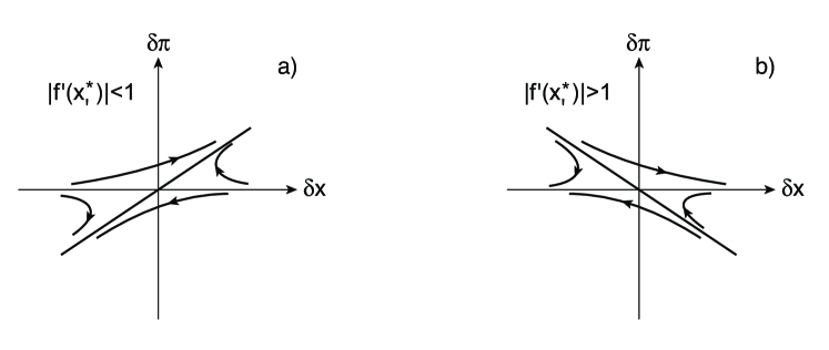
Figure 1: We depict the orbits in the vicinity of the deterministic hyperbolic fixed point ($x_{1}^{\ast}$,0). In a) we show the orbits in the case $|f^{\prime}(x_{1}^{\ast})|<1$, where the fixed point for the 1D map is stable. In b) we show the orbits for $|f^{\prime}(x_{1}^{\ast})|>1$; the fixed point for the 1D map is unstable.

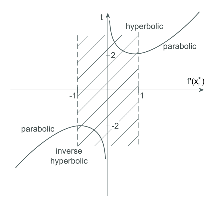
Figure 2: We plot the trace $t$ of the stability matrix $M$ as a function of the slope $f^{\prime}(x_{1}^{\ast})$ for the deterministic fixed point $(x_{1}^{\ast},0)$. The shaded area corresponds to the stability region of the 1D map.

For the noisy fixed point $(x^{\ast},\pi^{\ast})=(x_{2}^{\ast},\pi_{2})$, $\pi_{2}=x_{2}^{\ast}-f(x_{2}^{\ast})$, $f^{\prime}(x_{2}^{\ast})=1$, we obtain, setting $f^{\prime\prime}_{2}=f^{\prime\prime}_{2}(x_{2}^{\ast})$, trace, eigenvalues, and manifolds

$$t = 2-\pi_{2}^{\ast}f_{2}^{\prime\prime},$$ (49)

$$\lambda_{\pm} = \frac{\pi_{2}^{\ast}f_{2}^{\prime\prime}}{2}\pm\sqrt{\left(\frac{\pi_{2}^{\ast}f_{2}^{\prime\prime}}{2}\right)^{2}-\pi_{2}^{\ast}f_{2}^{\prime\prime}},$$ (50)

$$(\delta x,\delta\pi) \propto \left(1,\frac{\pi_{2}^{\ast}f_{2}^{\prime\prime}}{2}+\sqrt{\left(\frac{\pi_{2}^{\ast}f_{2}^{\prime\prime}}{2}\right)^{2}+\pi_{2}^{\ast}f_{2}^{\prime\prime}}\right),~{}~{}~{}~{}~{}~{}~{}~{}$$ (51)

$$(\delta x,\delta\pi) \propto \left(1,\frac{\pi_{2}^{\ast}f_{2}^{\prime\prime}}{2}-\sqrt{\left(\frac{\pi_{2}^{\ast}f_{2}^{\prime\prime}}{2}\right)^{2}+\pi_{2}^{\ast}f_{2}^{\prime\prime}}\right),~{}~{}~{}~{}~{}~{}~{}~{}$$ (52)

and the character of the fixed point depends on the specific map $f(x)$. In Fig. 3 we have depicted the orbits in the vicinity of the noisy fixed point in the two cases of a hyperbolic and elliptic fixed point. In Fig. 4 we have shown the trace $t$ as a function of $\pi_{2}^{\ast}f^{\prime\prime}(x_{2}^{\ast})$.

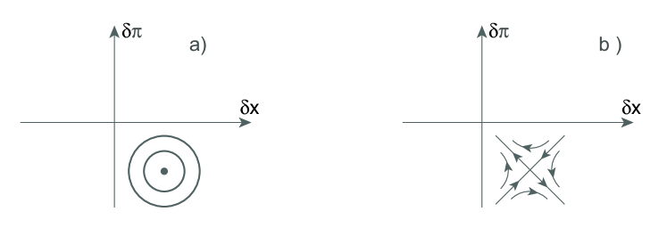
Figure 3: We show the orbits in the vicinity of the noisy fixed point. In a) we depict the elliptic case for $|\pi_{2}^{\ast}f^{\prime\prime}(x_{2}^{\ast})-2|<2$. In b) we show the hyperbolic case for $\pi_{2}^{\ast}f^{\prime\prime}(x_{2}^{\ast})>0$.

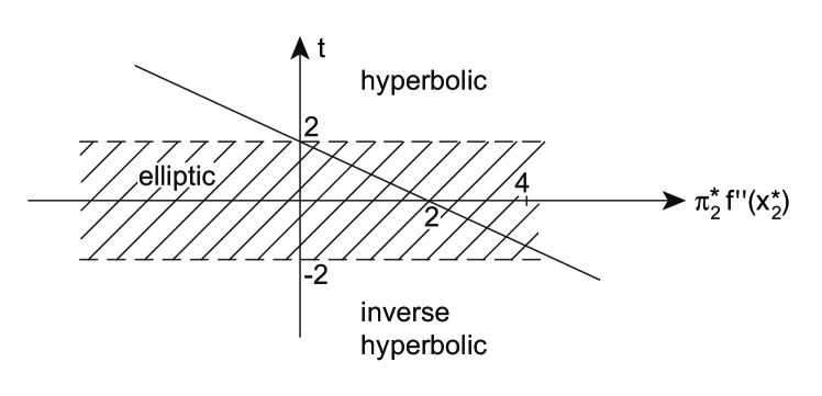
Figure 4: We plot the trace $t$ of the stability matrix $M$ as a function $\pi_{2}^{\ast}f^{\prime\prime}(x_{2}^{\ast})$. For $t>2$ the fixed point is hyperbolic, for $t<-2$ the fixed point in inverse hyperbolic. For $|t|<2$ the fixed point in elliptic.

II.4 Transition probabilities in the vicinity of the fixed points

Leaving aside for a moment the issue of the nonlinear breakdown of the orbit structure near the fixed point the weak noise scheme can be applied in order to determine the transition probabilities.

II.4.1 The deterministic fixed point

In the case of the deterministic fixed point $(x^{\ast},\pi^{\ast})=(x_{1}^{\ast},0)$, setting $a=f^{\prime}(x_{1}^{\ast})$ and inserting the initial and final values $\delta x_{1}$ and $\delta x_{N}$ and the time span $N$, the solution of the tangent map in Eq. (39) is

$$\delta x_{n}=\frac{\delta x_{N}(a^{n-1}-a^{-n+1})+\delta x_{1}(a^{N-n}-a^{-N+n})}{a^{N-1}-a^{-N+1}},$$

(53)

$$\delta\pi_{n}=(a^{2}-1)\frac{\delta x_{N}a^{1-n}-\delta x_{1}a^{N-n}}{a^{N-1}-a^{-N+1}},$$ (54)

describing an orbit from $\delta x_{1}$ to $\delta x_{N}$ in time $N$ with $\delta\pi_{n}$ as a slaved variable.

For $|a|=|f^{\prime}(x_{1})|<1$ the fixed point is stable on the transient invariant manifold $\delta\pi_{n}=0$. In the absence of noise the motion on the manifold corresponds to damping, i.e., the 1D map is line contracting. In the presence of noise for $\delta\pi_{n}\neq 0$ the orbits escape from the fixed point and approaches the stationary invariant manifold $\delta\pi_{n}=(1-a^{2})\delta x_{n}$; this is the scenario depicted in Fig. 1 a). In the continuum limit this behavior corresponds to the flow for the noise-driven overdamped oscillator discussed in Ref. Fogedby (1999).

For $|a|>1$ the fixed point is unstable on the invariant manifold $\delta\pi_{n}=0$. However, we note that in this case $\delta\pi_{n}\rightarrow 0$. The fixed point is attractive along the invariant noisy manifold $\delta\pi_{n}=-(a^{2}-1)\delta x_{n}$; the orbit structure is depicted in Fig. 1 b). In the vicinity of the hyperbolic fixed point the orbit slows down and an orbit from $\delta x_{1}$ to $\delta x_{N}$ in time $N$ must pass asymptotically through the fixed point for $N\rightarrow\infty$.

In order to evaluate the transition probability from $\delta x_{1}$ to $\delta x_{N}$ in time $N$ we insert $\delta\pi_{n}=\delta p_{n-1}$ in the expression for the action in Eq. (9). Performing the sum yields the action

$$S=\frac{1}{2}(a^{2}-1)(1-a^{-2N})\left(\frac{\delta x_{N}-\delta x_{1}a^{N-1}}{a^{N-1}-a^{-N+1}}\right)^{2},$$ (55)

and from Eqs. (7) and (8) the normalized transition probability

$$P(\delta x_{1}\rightarrow\delta x_{N},N)=\Omega(N)^{-1}\times\exp\left[-\frac{(a^{2}-1)(1-a^{-2N})}{2\Delta}\left(\frac{\delta x_{N}-\delta x_{1}a^{N-1}}{a^{N-1}-a^{-N+1}}\right)^{2}\right],$$ (56)

with dynamic partition function

$$\Omega(N)=(a^{N-1}-a^{-N+1})\left(\frac{2\pi\Delta}{(a^{2}-1)(1-a^{-2N})}\right)^{1/2}.$$ (57)

In the long time limit $N\rightarrow\infty$ the behavior of $S$, $P$, and $\Omega$ depends on $a=f^{\prime}(x_{1}^{\ast})$. For $|a|<1$ we obtain

$$S\rightarrow\frac{1}{2}(1-a^{2})\left(\frac{\delta x_{N}}{a}\right)^{2},$$ (58)

and thus the stationary distribution

$$P_{\text{st}}\propto\exp\left[-\frac{1}{2\Delta}(1-a^{2})\left(\frac{\delta x_{N}}{a}\right)^{2}\right].$$ (59)

II.4.2 The noisy fixed point

The noisy fixed point $(x^{\ast},\pi^{\ast})=(x_{2}^{\ast},x_{2}^{\ast}-f(x_{2}^{\ast}))$, $f^{\prime}(x_{2}^{\ast})=1$ is elliptic for $|\pi_{2}^{\ast}f^{\prime\prime}(x_{2}^{\ast})-2|<2$ and hyperbolic for $|\pi_{2}^{\ast}f^{\prime\prime}(x_{2}^{\ast})-2|>2$. In the hyperbolic case the discussion in the deterministic case applies, we leave the details to the reader. In the elliptic case the complex eigenvalues are determined by Eq. (50). The orbits are periodic and given by

$$\delta x_{n}=A\cos(\omega n+\psi_{1}),$$ (60)

$$\delta\pi_{n}=B\cos(\omega n+\psi_{2}),$$ (61)

where the frequency $\omega$ is given by

$$\tan\omega=\frac{2-\pi_{2}^{\ast}f^{\prime\prime}_{2}}{\sqrt{\pi_{2}^{\ast}f^{\prime\prime}_{2}(4-\pi_{2}^{\ast}f^{\prime\prime}_{2})}}.$$ (62)

In the hyperbolic case, the long time orbits near the fixed point permits a derivation of the transition probability as in the case of the deterministic fixed point on the $\pi=0$ manifold. In the elliptic case, the finite time orbits also allow an evaluation of $P$; we shall, however, not pursue this analysis here.

Summarizing, the 2D map describing the noisy 1D map within the nonperturbative weak noise approach is characterized by at least two fixed points. The noiseless deterministic fixed point is hyperbolic. The character of the noisy fixed point(s) depends on the magnitude of $\pi_{2}^{\ast}f^{\prime\prime}(x_{2}^{\ast})$. In the vicinity of the hyperbolic fixed point the orbits slow down and we can derive a stationary probability distribution in the linear regime. Near the elliptic fixed point the finite time orbits only yield the short time character of the probability distributions.

Owing to the nonlinear character of the 2D map we anticipate that the orbit structure near the hyperbolic fixed point breaks down due to heteroclinic intersections and the formations of foliations. In the vicinity of the elliptic fixed point we expect to encounter the dissolution of the KAM tori into cantori and chaotic seas with Arnold diffusion Ott (1993); Reichl (1987). Some of these features will be investigated in more detail in the next section on the noisy logistic map.

III 1D Noisy Maps

In this section we embark on a discussion of specific noise-driven 1D maps which in the absence of noise exhibits nonlinear behavior such as period doubling and transitions to chaotic behavior.

III.1 The linear map

It is instructive to briefly consider the linear map

$$x_{n+1}=rx_{n},$$ (63)

with control parameter $r$. The Jacobian $J=dx_{n+1}/dx_{n}=r$ and for $r<1$ the map is length-shrinking with a stable fixed point at $x^{\ast}=0$; for $r=0$ the map is length-preserving with a line of fixed points. For $r>0$ the map is length-expanding, the fixed point at $x^{\star}$ is unstable and the orbit recedes to infinity. In the presence of noise we obtain the noisy map

$$x_{n+1}=rx_{n}+\xi_{n},$$ (64)

corresponding to the 2D area-preserving map

$$x_{n+1}=rx_{n}+r^{-1}\pi_{n},$$ (65)

$$\pi_{n+1}=r^{-1}\pi_{n}.$$ (66)

This map possesses a hyperbolic fixed point at $(x^{\ast},\pi^{\ast})$ and the discussion in Sec. II applies.

III.2 The logistic map

We now turn to the well-known 1D logistic map

$$x_{n+1}=rx_{n}(1-x_{n}),$$ (67)

which has fixed points at $x^{\ast}=0$ and $x^{\ast}=1-1/r$. For $r>3$ the fixed point bifurcates to period-2 fixed points and in the regime $3<r<r_{c}$, $r_{c}\approx 3.57$ the map passes through a period-doubling scenario exhibiting universal scaling behavior Feigenbaum (1978, 1979).

In the presence of noise we have the stochastic map

$$x_{n+1}=rx_{n}(1-x_{n})+\xi_{n},$$ (68)

and the associated area preserving 2D map

$$x_{n+1}=rx_{n}(1-x_{n})+\frac{\pi_{n}}{r(1-2x_{n})},$$ (69)

$$\pi_{n+1}=\frac{\pi_{n}}{r(1-2x_{n})}.$$ (70)

Since $f(x)=rx(1-x)$, $f^{\prime}(x)=r(1-2x)$, and $f^{\prime\prime}(x)=-2r$ and according to the general discussion in Sec. II the 2D map has two deterministic fixed points on the $x$- axis and a noisy fixed point in the lower half $x-\pi$ plane:

$$(x^{\ast},\pi^{\ast})=(0,0),~{}~{}~{}~{}~{}~{}~{}~{}~{}~{}~{}~{}~{}~{}~{}~{}~{}~{}~{}~{}~{}~{}~{}~{}~{}~{}~{}~{}~{}~{}~{}~{}~{}\text{(FP1)}$$ (71)

$$(x^{\ast},\pi^{\ast})=(1-1/r,0),~{}~{}~{}~{}~{}~{}~{}~{}~{}~{}~{}~{}~{}~{}~{}~{}~{}~{}~{}~{}~{}~{}~{}~{}~{}\text{(FP2)}$$ (72)

$$(x^{\ast},\pi^{\ast})=((r-1)/2r,-(1-r)^{2}/4r).~{}~{}~{}~{}~{}\text{(FP3)}$$ (73)

The trace and eigenvalues characterizing the stability and properties of the fixed points are given by Eqs. (43) and (44); likewise, the invariant manifolds follow from $(\delta x,\delta\pi)\propto(1,-(f^{\prime 2}-\pi f^{\prime\prime}-f^{\prime}\lambda_{\pm}))$. The fixed point form a triad. The traces associated with the fixed points are given by

$$t_{1}=r+\frac{1}{r},$$ (74)

$$t_{2}=2-r+\frac{1}{2-r},$$ (75)

$$t_{3}=2-\frac{(1-r)^{2}}{2}.$$ (76)

We can now read off the character of the fixed points and establish the correspondence with the bifurcations of the noiseless 1D map. First, we infer that for all $r>0$ (we only consider positive $r$) the deterministic fixed points FP1 and FP2 on the $x$-axis are hyperbolic, whereas the noisy fixed point is elliptic for $r<r_{t}$ and hyperbolic for $r>r_{t}$, where $r_{t}=1+\sqrt{8}\approx 3.8284$ corresponds to the period 3 tangent bifurcation for the 1D map.

Let us first concentrate at the first period doubling point at $r=3$. The Jacobian matrix (39) for the 2D map of the logistic equation is of the form

$$M=\left(\begin{array}[]{cc}r-2rx^{\ast}+\frac{2\pi^{\ast}}{r(1-2x^{\ast})^{2}}&\frac{1}{r-2rx^{\ast}}\\ \frac{2\pi^{\ast}}{r(1-2x^{\ast})^{2}}&\frac{1}{r-2rx^{\ast}}\end{array}\right).$$ (79)

For the fixed point FP2 (where $\pi^{\ast}=0$) at $r=3$ it then takes the form

$$M=\left(\begin{array}[]{cc}-1&-1\\ 0&-1\end{array}\right).$$ (82)

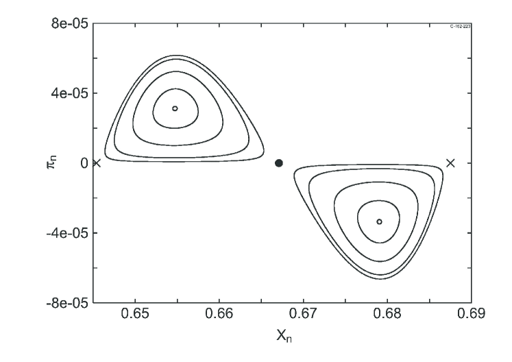
Figure 5: The phase plane $(x_{n},\pi_{n})$ for $r=3.004$ just above the period-doubling into the two-cycle. The black dot is the now (hyperbolic) unstable fixed point; the crosses are the two-cycle on the x-axis and the KAM curves encircle the elliptic two-cycle.

This corresponds to a degenerate node where the two eigendirections coincide along the x-axis. For $r<3$ the eigenvalues are $\lambda_{1}<-1$ and $\lambda_{2}>-1$, respectively. At $r=3$ the eigenvalues collide in -1 signalling that two period-doublings are about to take place. In Fig. 5 we show this behavior just above $r=3$, at $r=3.004$. The black dot represents the (unstable) fixed point FP2, which seen in the 2D plane now is a hyperbolic fixed point. The crosses determines the “usual” stable period two cycle. Simultaneously, a period two cycle of elliptic points has been spinning off. Initially, along the eigendirection in the x-axis but quickly moving nonlinearly into the plane. We have numerically followed the upper elliptic two-cycle point as far as we could for increasing $r$. The KAM surfaces around it gradually dissolves and to the best of our knowledge without the cycle point undergoes further period-doubling’s. Fig. 6 shows this two-cycle point at $r=3.608$, with only a few remaining KAM surfaces around it, seen on a tiny scale.

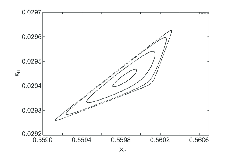
Figure 6: One of the elliptic two-cycle points for $r=3.6084$ in the “chaotic sea” of the energy surface. The KAM surfaces remain only on very small scales close to the cycle point.

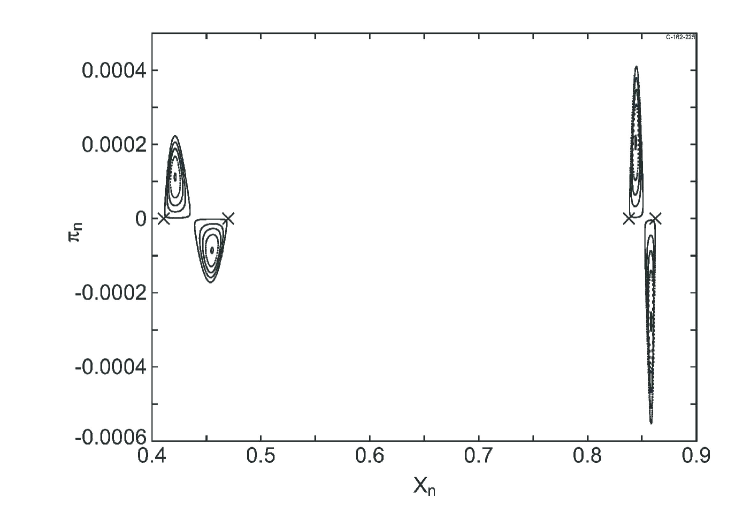
Figure 7: The behavior at $r=3.462$ just above the period-doubling into the four-cycle. Note, the usual stable four-cycle on the axis and the associated elliptic four-cycle.

Furthermore, for increasing values of $r$, what happens is a continuous spinning off of elliptic cycles in close association with the standard period-doubling sequence on the x-axis. We show this in Fig. 7 (for the parameter value $r=3.462$) for the period-doubling to the four-cycle occurring at $r\approx 3.449$. Note again the normal stable four-cycle, represented by crosses, on the x-axis and the associated four-cycle of elliptic points in the plane. To substantiate this picture even further, we finally study the behavior just above the period-doubling into the stable eight-cycle. At $r=3.55$, this is shown in Fig. 8 with the same structure of the stable eight-cycle on the axis with the elliptic eight-cycle in the plane. We thus conclude, that this process will continue in the same fashion, with elliptic $2^{n}$ cycle moving away from the x-axis into the plane at each bifurcation point.

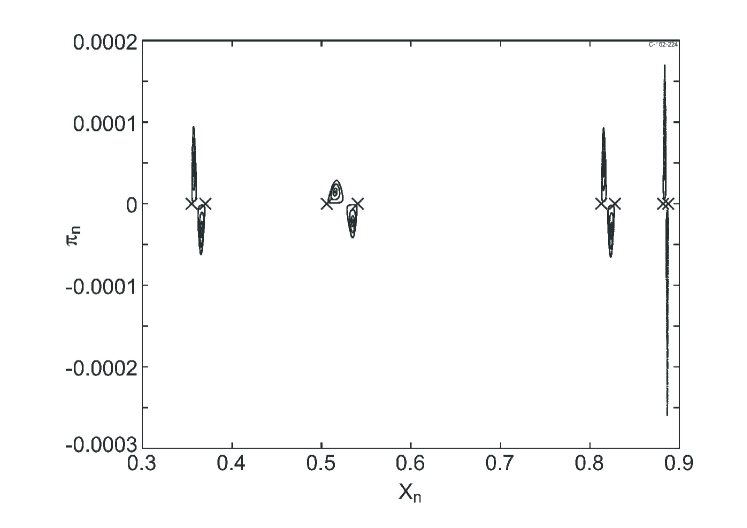
Figure 8: The phase plane at $r=3.55$ above the period-doubling into the eight-cycle, where the crosses indicate the stable eight-cycle.

For $r>r_{c}$ the 1D map approaches a strange attractor with positive Liapunov exponent. In the 2D map this is reflected by orbits approaching the x-axis subject to infinitely many foliations in order to preserve the area.

IV Summary and conclusion

We have attacked the old problem of noise in 1D maps, in particular the logistic equation, in a new way. Starting out with a discrete version of the standard Langevin equation, we apply a nonperturbative weak noise approach to map the stochastic equation onto a deterministic 2D map. This map is area-preserving and the added dimension plays the role of the noise field. We have derived general properties of this 2D map and applied it to two well know systems, the trivial linear map and the logistic map. In both cases we find, that in addition to the standard fixed points in the usual variable, there are additional fixed points and higher order cycles out in the plane of finite noise amplitude. These fixed and cycle points are either hyperbolic or elliptic. In the case of the logistic map we find that each standard period-doubling on the x-axis is always associated with a period-doubling out in the plane. These cycles in the plane of order $2^{n}$ are born as elliptic points moving away from the cycle points on the x-axis at the bifurcation points.