Thermodynamic formalism for the Lorentz gas with open boundaries in $d$ dimensions

Abstract

A Lorentz gas may be defined as a system of fixed dispersing scatterers, with a single light particle moving among these and making specular collisions on encounters with the scatterers. For a dilute Lorentz gas with open boundaries in $d$ dimensions we relate the thermodynamic formalism to a random flight problem. Using this representation we analytically calculate the central quantity within this formalism, the topological pressure, as a function of system size and a temperature-like parameter $\beta$. The topological pressure is given as the sum of the topological pressure for the closed system and a diffusion term with a $\beta$-dependent diffusion coefficient. From the topological pressure we obtain the Kolmogorov-Sinai entropy on the repeller, the topological entropy, and the partial information dimension.

I Introduction

In the seventies of the last century Sinai, Ruelle, and Bowen developed a formalism for calculating dynamical properties of chaotic dynamical systems Sinai (1972); Ruelle (1978); Bowen (1975). This formalism resembles very much Gibbs ensemble theory and therefore was given the name thermodynamic formalism. From a partition function defined as an integral over phase space of a particular weight function, one may derive several dynamical quantities, such as the Kolmogorov-Sinai (KS) entropy, the topological entropy, the escape rate, or the partial information dimension Eckmann and Ruelle (1985); Beck and Schlögl (1993).

Although the power of this formalism has been widely recognized, there are only few examples so far of physically interesting systems for which the topological pressure and related functions could be evaluated explicitly. One such system is the dilute random Lorentz gas. Generally spoken a Lorentz gas is a system consisting of fixed dispersing scatterers, among which a single light particle (or alternatively a cloud of mutually non-interacting light particles) moves about, making specular collisions on each encounter with a scatterer. The scatterers may either be placed on a periodic lattice or at random positions in space. Usually the scatterers are taken to be disks, in $d=2$, spheres, in $d=3$, or hyperspheres, for $d>3$. If these are placed on a periodic lattice the resulting system is also known as the Sinai billiard Sinai (1970). In fact this is also the model Lorentz Lorentz (1905) had in mind originally for describing the transport of conduction electrons in metals (still in the pre-quantum era). However the kinetic equation he proposed to describe this system, presently known as the Lorentz-Boltzmann equation (see for instance Hauge (1999); Dorfman (1999); van Beijeren (1982)), in fact is more appropriate for the model with random scatterer locations, at low density of scatterers. The Lorentz-Boltzmann equation and some of its generalizations to higher densities van Leeuwen and Weijland (1982); Weyland and van Leeuwen (1982); Ernst and Weyland (1982) allow for analytic calculations of transport coefficients and other fundamental nonequilibrium properties.

Recently, several dynamical properties have been calculated analytically for open and closed random Lorentz gases by using an extended Lorentz-Boltzmann equation approach van Beijeren and Dorfman (1995); van Beijeren et al. (1998, 2000); de Wijn and van Beijeren (2004). Van Beijeren and Dorfman van Beijeren and Dorfman (2002) alternatively used the thermodynamic formalism to calculate the topological pressure and related quantities for a dilute d-dimensional random Lorentz gas in equilibrium. For 2 dimensions this was extended by the present authors Mülken and van Beijeren (2004) to the case of a dilute random Lorentz gas under the combined actions of a driving field and an isokinetic gaussian thermostat.

II thermodynamic formalism

In chaos theory a central role is played by the time evolution of infinitesimal volumes in phase space. For chaotic systems such a volume element will grow in some directions and shrink in others. The factor by which the projection of the volume element onto its unstable (expanding) manifold increases over a time $t$ is called the stretching factor. For an infinitesimal volume centered originally around the phase point $(\bm{r},\bm{v})$ we will denote its value as $\Lambda(\bm{r},\bm{v},t)$. Similarly, the contraction factor is the factor by which the projection onto the stable (contracting) manifold decreases over time $t$. In analogy to the Gibbs ensemble formalism of statistical mechanics, we may define a dynamical partition function $Z(\beta,t)$ as a weighted integral over phase space. For closed systems, indicated by a subscript $0$, points in phase space are weighted by powers of their stretching factor, according to

$$Z_{0}(\beta,t)=\int d\mu(\bm{r},\bm{v})\left[\Lambda(\bm{r},\bm{v},t)\right]^{1-\beta},$$ (1)

where the integration is over an appropriate stationary measure. In systems with escape, phase space trajectories are removed from the ensemble if they hit an absorbing boundary. In this case the definition of the dynamical partition function has to be generalized to

$$Z(\beta,t)=\int d\mu(\bm{r},\bm{v})\left[\Lambda(\bm{r},\bm{v},t)\right]^{1-\beta}\chi_{tr}(\bm{r},\bm{v},t),$$ (2)

with $\chi_{tr}(\bm{r},\bm{v},t)=0$ if the trajectory starting from $(\bm{r},\bm{v})$ at time 0 hits the absorbing boundary before time $t$ and $\chi_{tr}(\bm{r},\bm{v},t)=1$ otherwise. In our analogy to statistical mechanics the parameter $\beta$ behaves like an inverse temperature and as the analogon of the Helmholtz free energy we obtain the topological pressure $P(\beta)$ as

$$P(\beta)=\lim_{t\to\infty}\frac{1}{t}\ln Z(\beta,t).$$ (3)

The dynamical entropy function $h(\beta)$ is given by the Legendre transform of $P(\beta)$ as,

$$h(\beta)=P(\beta)-\beta P^{\prime}(\beta),$$ (4)

where $P^{\prime}(\beta)=dP(\beta)/d\beta$. For special values of $\beta$ the dynamical entropy function can be identified with dynamical properties, because for long times we have $\Lambda\simeq\exp(t\sum^{+}_{i}\lambda_{i})$, where $\sum^{+}_{i}\lambda_{i}$ is the sum of all positive Lyapunov exponents $\lambda_{i}$. Specifically, $h(\beta)$ equals the topological entropy $h_{\rm top}$ for $\beta=0$ and the KS entropy $h_{KS}$ for $\beta=1$. If the system is closed, the KS entropy equals the sum of positive Lyapunov exponents because $P_{0}(1)=0$, as follows directly from Eqs. (1) and (3).

However, for open systems $P(1)=-\gamma$, where $\gamma$ is the asymptotic escape rate. The relationship $P^{\prime}(1)=\sum^{+}_{i}\lambda_{i}$ still holds, but now the Lyapunov exponents are defined on the repeller, i.e. the subset of phase space from which no trajectories escape. The point where $P(\beta)$ intersects the $\beta$-axis can be related to the partial Hausdorff dimension, which is a fractal dimension of a line across the stable manifold of the attractor. Another fractal dimension associated with the topological pressure is the partial information dimension which is given by the intersection point with the $\beta$-axis of the tangent to $P(\beta)$ at $P(1)$. For the closed system both dimensions coincide and are equal to $1$.

III Dynamical partition function for the open Lorentz gas in $d$ dimensions

In this section we will calculate $Z(\beta,t)$ for a dilute random open Lorentz gas in $d$ dimensions, with $N$ fixed (hyper)spherical scatterers of radius $a$ distributed randomly inside a finite volume $V$. In addition there is one point particle moving with velocity $v$ along straight lines between specular collisions with the scatterers. If the particle leaves $V$ it escapes. ”Dilute” implies the condition $na^{d}\ll 1$, with the density $n=N/V$.

The condition of diluteness allows us to approximate the dynamics of the light particle as a random flight, in which each trajectory between subsequent collisions is sampled from an exponential distribution of free path lengths and the collision parameters of each collision are sampled from a distribution corresponding to a homogeneous bundle hitting the scatterer. In other words: all effects resulting from recollisions are completely ignored. Under these approximations the dynamical partition function may be rewritten as

$$Z(\beta,t) = e^{P_{0}(\beta)t}\int d\bm{r}\int d\bm{v}\delta(|\bm{v}|-v_{0})\sum_{l=0}^{\infty}\int_{0}^{\infty}dt_{1}\cdots dt_{l}\int d\mu(\hat{\sigma}_{1})\cdots d\mu(\hat{\sigma}_{l})$$ (5)

$$\Theta\left(t-\sum_{i=1}^{l}t_{i}\right)\exp\left[-\left((\nu_{d}+P_{0}(\beta))(t-\sum_{i=1}^{l}t_{i})\right)\right]\chi\left(\bm{r}_{l}+\bm{v}_{l}^{\prime}(t-\sum_{i=1}^{l}t_{i})\right)\prod_{j=1}^{l}W(\hat{\sigma}_{j},t_{j})\chi(\bm{r}_{j}).$$

Here $P_{0}$ is the topological pressure for the closed Lorentz gas at the same density in equilibrium; $\hat{\sigma}_{i}$ denotes the collision normal at the $i$th collision and $d\mu(\hat{\sigma})$ denotes the probability measure for scattering with collision normal $\hat{\sigma}$; $\Theta(x)$ denotes the unit step function, i.e. $\Theta(x)=1$ for $x\geq 0$ and $\Theta(x)=0$ for $x<0$; $\nu_{d}\equiv 1/\bar{\tau}_{d}$ is the average collision rate, given for dimension $d$ as van Beijeren and Dorfman (2002)

$$\nu_{d}=\frac{2nva^{d-1}\pi^{\frac{d-1}{2}}}{(d-1)\Gamma\left(\frac{d-1}{2}\right)},$$ (6)

$\bm{r}_{j}$ is the position of the light particle at the $j$th collision, and $\chi(\bm{r})$ is the characteristic function satisfying $\chi(\bm{r})=1$ for $\bm{r}$ inside $V$ and 0 otherwise. We implicitly assumed that the boundary is not concave, so if both $\chi(\bm{r}_{j})$ and $\chi(\bm{r}_{j+1})$ equal unity the same is true for the characteristic function of all points in between. In addition, $\bm{v}_{l}^{\prime}$ is the velocity of the light particle just after the $l$th collision. Finally, $W(\hat{\sigma},t)$ is an effective free flight transition rate, defined as

$$W(\hat{\sigma},t)=\nu_{d}e^{-(P_{0}(\beta)+\nu_{d})t}\left[\Lambda_{d}(\theta,t)\right]^{1-\beta}.$$ (7)

Here the stretching factor is given by van Beijeren et al. (1998); de Wijn and van Beijeren (2004)

$$\Lambda_{d}(\theta,t)=\left(\frac{2vt}{a}\right)^{d-1}(\cos\theta)^{d-3},$$ (8)

where $\theta$ is the scattering angle, defined through $\cos\theta=-\hat{v}\cdot\hat{\sigma}$, with $\hat{v}$ the unit vector along the velocity of the light particle before the collision, see Fig. 1.

Figure 1: Sketch of a trajectory in two dimensions of the light particle starting form the initial point and following the first two collisions.

Since in Eq. (7) the only dependence of the integrand on $\hat{\sigma_{j}}$ occurs through $\cos\theta_{j}$, the integrations over $d\mu(\hat{\sigma_{j}})$ may be reduced as

$$\int d\mu(\hat{\sigma_{j}})\to(d-1)\int_{0}^{\pi/2}d\theta_{j}\cos\theta_{j}\sin^{d-2}\theta_{j}.$$

Note that in Eq. (7) the actual free flight distribution has been changed to an effective free flight distribution by multiplication by the $(1-\beta)$th power of the stretching factor and by the factor $\exp(-P_{0}(\beta)t)$. Similarly, the distribution of collision normals has been changed to an effective distribution. Indeed, after this rearrangement the integral of $W(\hat{\sigma},t)$ over $d\mu(\hat{\sigma})$ and positive $t$ equals unity van Beijeren and Dorfman (2002). The second moments of both time and displacement for the effective distribution $W(\hat{\sigma},t)$ are well-defined, and the resulting effective random flight process for given initial direction gives rise to a convergent average displacement after $n$ steps in the limit $n\to\infty$. Therefore, on large time and length scales it leads to a normal diffusion process, with a $\beta$-dependent diffusion coefficient $D(\beta)$.

On division of the logarithm of Eq. (5) by $t$ the first factor just simply reduces to $P_{0}(\beta)$. The contribution from the remaining factor may be interpreted, up to a normalization factor, as the average survival probability of an initially homogeneously distributed cloud of light particles of equal energy, under the effective random flight process with absorbing boundaries described above. Since on large time and length scales this becomes an effective diffusion process, this survival probability will behave as $\exp(-k_{0}^{2}D(\beta)t)$ for long times, with $k_{0}$ determined by the geometry of the system and to some extent by the boundary conditions on the random flight process. Therefore the second contribution is of the form $-k_{0}^{2}D(\beta)$. Combination of these two brings us to the main result of this paper: the topological pressure for the dilute open random Lorentz gas may be expressed as

$$P(\beta)=P_{0}(\beta)-k_{0}^{2}D(\beta).$$ (9)

What remains to be done now is finding an explicit expression for $D(\beta)$ as a function of both $\beta$ and $d$. This task is not particularly hard. The Green-Kubo expression for the diffusion coefficient as a time integral of the velocity autocorrelation function gives rise to

$$D(\beta) = \frac{1}{d}\int_{0}^{\infty}dt\ \langle\vec{v}(0)\cdot\vec{v}(t)\rangle$$ (10)

$$= \frac{v^{2}}{d}\left[\langle\tau_{0}\rangle+\sum_{l=1}^{\infty}\langle\cos(\pi-2\theta)\rangle^{l}\langle\tau\rangle\right].$$

The first term is the contribution from free flights from the initial time until the first collision, the next terms result from free flights between the $l$th and $(l+1)$th collisions. Since the collision cross-sections are isotropic and all collisions are uncorrelated, the average direction of the velocity after the $l$th collision is proportional to $\langle\cos(\pi-2\theta)\rangle^{l}$. Then we obtain from Eqs. (5) and (7) the time averages

$$\langle\tau_{0}\rangle = \frac{\langle\tau^{2}\rangle}{2\langle\tau\rangle}=\frac{1}{\nu_{d}+P_{0}(\beta)}\left[1+\frac{(d-1)(1-\beta)}{2}\right],$$ (11)

$$\langle\tau\rangle = \frac{1}{\nu_{d}+P_{0}(\beta)}\left[1+(d-1)(1-\beta)\right],$$ (12)

together with the angular average

$$\langle\cos(\pi-2\theta)\rangle=\frac{-\beta(3-d)}{2(d-1)+\beta(3-d)}.$$ (13)

To understand the first equality in Eq. (11) one should realize that the probability of finding the initial time on a free-time stretch of length $\tau$ is proportional to $\tau$ and that the average time until the first collision under these conditions is just $\tau/2$. Furthermore Eqs. (11) and (12) only make sense for $\beta<d/(d-1)$ since for larger $\beta$-values the effective free-time distribution shows a divergence, see Eqs. (7) and (8). Similarly Eq. (13) has to be restricted to the range $\beta>-1$, for $d=2$, respectively $\beta<(d-1)/(d-3)$ for $d\geq 4$ (for $d=3$ there are no restrictions).

The topological pressure for the closed Lorentz gas in equilibrium is obtained from the first pole of the Laplace transform of the dynamical partition function van Beijeren and Dorfman (2002); Mülken and van Beijeren (2004) and for the closed Lorentz gas in equilibrium it reads

$$P_{0}(\beta) = \nu_{d}\left\{\left[\frac{d-1}{2}\left(\frac{2v}{a\nu_{d}}\right)^{(d-1)(1-\beta)}\Gamma\left(d+\beta-d\beta\right)\right.\right.$$ (14)

$$\times\left.\left.\frac{\Gamma\left(\frac{d-1}{2}\right)\Gamma\left(\frac{d-1+\beta(3-d)}{2}\right)}{\Gamma\left(d-1+\frac{\beta(3-d)}{2}\right)}\right]^{\frac{1}{d+\beta-d\beta}}-1\right\}.\$$

Note that for the closed Lorentz gas in equilibrium the topological pressure vanishes for $\beta=1$. Now $D(\beta)$ is given by

$$D(\beta) = \frac{v^{2}}{d(\nu_{d}+P_{0}(\beta))}\left[1+\frac{(d-1)(1-\beta)}{2}\right.$$ (15)

$$\left.-\frac{[1+(d-1)(1-\beta)]\beta(3-d)}{2[d-1+\beta(3-d)]}\right].$$

From this we can easily get the normal diffusion coefficient by setting $\beta=1$, i.e.,

$$D(1)=\frac{v^{2}(d+1)}{4d\nu_{d}}.$$ (16)

IV Other dynamical properties

As mentioned before, from the dynamical partition function we may obtain several other dynamical characteristics of our system. For $\beta=1$ the topological pressure equals minus the escape rate $\gamma$, thus we have $\gamma=k_{0}^{2}D(1)$. From Eqs. (4) and (9) we obtain the dynamical entropy function $h(\beta)$ as

$$h(\beta)=h_{0}(\beta)-k_{0}^{2}\left[D(\beta)-\beta D^{\prime}(\beta)\right],$$ (17)

with $D^{\prime}(\beta)=dD(\beta)/d\beta$ and $h_{0}(\beta)$ the entropy function for the closed Lorentz gas in equilibrium.

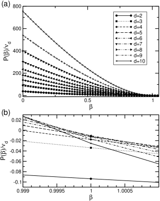
Figure 2: (a) Topological pressure divided by the collision frequency as a function of $\beta$ for different dimensions $d$, with the parameter choice $a=1$, $v=1$, $n=0.001$, and $k_{0}=0.001$. (b) A close-up of this for $\beta$-values around 1.

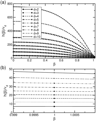
Figure 3: (a) Dynamical entropy divided by the collision frequency, as function of $\beta$ for different dimensions $d$ and with the parameter choice $a=1$, $v=1$, $n=0.001$, and $k_{0}=0.001$. (b) A close-up of this for $\beta$-values around 1.

Figures 2 and 3 show the topological pressure and the dynamical entropy, respectively, divided by the collision frequency, as functions of $\beta$ for different dimensions $d$. As expected, $P(\beta)$ is negative for $\beta=1$ because $P(1)=-\gamma$, see the inset of Fig. 2. Furthermore, $P(\beta)$ is a convex function for all dimensions considered. Since $k_{0}\ll 1$ for large systems, the deviations of $P(\beta)$ and $h(\beta)$ from their equilibrium values are small.

The logarithms of the prefactors of the correction terms in Eqs. (9) and (17) proportional to $k_{0}^{2}$ are plotted in Fig. 4. For $P(\beta)$ this prefactor is $D(\beta)$, which is always positive within the allowed ranges of $\beta$ and $d$. As can be seen from Eq. (15) $D(\beta)$ diverges at a pole located at $\beta=(d-1)/(d-3)$. In Fig. 4(b) the logarithm of the absolute value of the correction term for the dynamical entropy is plotted because the prefactor changes sign at $\beta\approx 0.4$, see inset Fig. 4(b). Thus the correction to the topological entropy at $\beta=0$ will be negative while the one for the KS-entropy at $\beta=1$ will be positive (see also the discussion).

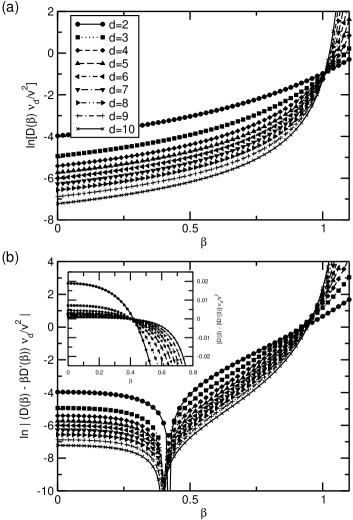
Figure 4: Natural logarithms of the correction terms proportional to $k_{0}^{2}$ of (a) the topological pressure, see Eq. (9), and (b) the absolute value of the dynamical entropy, see Eq. (17), as a function of $\beta$ for different dimensions $d$. The inset in (b) shows a close-up of $\left[D(\beta)-\beta D^{\prime}(\beta)\right]$ around $\beta=0.4$, where this function crosses zero. All results are for $a=1$, $v=1$, and $n=0.001$

The KS entropy for general $d$ for the open Lorentz gas is given by

$$h(1)=h_{KS}=h^{0}_{KS}-k_{0}^{2}D(1)\left[\frac{d+1}{2}-\frac{h^{0}_{KS}}{\nu_{d}}\right],$$ (18)

where $h^{0}_{KS}$ is the equilibrium value of the KS entropy for the closed Lorentz gas in $d$ dimensions. The specific form of this as a function of $d$ reads

$$h^{0}_{KS} = \nu_{d}(1-d)\left[{\cal C}-\ln\left(\frac{2v}{a\nu_{d}}\right)\right]$$ (19)

$$+\frac{\nu_{d}}{2}(3-d)\left[{\cal C}+\Psi\left(\frac{d+1}{2}\right)\right],$$

with ${\cal C}$ Euler’s constant and $\Psi(x)$ the digamma function Gradshteyn and Ryzik (1965).

For $d=2$ and $d=3$ we can compare our results to previous calculations based on an extended Lorentz-Boltzmann equation approach van Beijeren et al. (2000). From Eq. (19) we get the KS entropy for $d=2$ as

$$h_{KS}=h^{0}_{KS}-k_{0}^{2}\frac{3v^{2}}{8\nu_{2}}\left[\frac{3}{2}-\frac{h^{0}_{KS}}{\nu_{2}}\right].$$ (20)

$h^{0}_{KS}$ is given by the one positive Lyapunov exponent in equilibrium

$$h^{0}_{KS}=\lambda_{0}^{+}=\nu_{2}\left[1-{\cal C}-\ln\left(\frac{a\nu_{2}}{v}\right)\right].$$ (21)

The KS entropy for $d=3$ follows as

$$h_{KS}=h^{0}_{KS}-k_{0}^{2}\frac{v^{2}}{3\nu_{3}}\left[2-\frac{h^{0}_{KS}}{\nu_{3}}\right].$$ (22)

Here, $h^{0}_{KS}$ is given by the sum of the positive Lyapunov exponents in equilibrium

$$h^{0}_{KS}=\sum_{i}\lambda^{+}_{0,i}=2\nu_{3}\left[\ln\left(\frac{2v}{a\nu_{3}}\right)-{\cal C}\right].$$ (23)

As one should expect, Eqs. (20-23) are in agreement with the previous calculation.

From the escape rate formalism Gaspard and Nicolis (1990) we know that the KS entropy equals the sum of positive Lyapunov exponents minus the escape rate. Note that here the Lyapunov exponents are defined on the repeller. Furthermore, for $\beta=1$ the topological pressure equals the escape rate $\gamma$ and this can be expressed for the open Lorentz gas as $\gamma=k_{0}^{2}D(1)$. Therefore, we have an equation for the sum of positive Lyapunov exponents of the open Lorentz gas,

$$\sum_{i}\lambda_{i}^{+} = \sum_{i}\lambda_{0,i}^{+}+k_{0}^{2}D^{\prime}(1)$$ (24)

$$= h^{0}_{KS}+k_{0}^{2}D(1)\left[\frac{1-d}{2}+\frac{h^{0}_{KS}}{\nu_{d}}\right].$$ (25)

The correction term proportional to the diffusion coefficient is always positive, because for low densities the term $\ln(2v/a\nu_{d})\gg 1$ in Eq. (23) dominates. Hence, the sum of positive Lyapunov exponents is always larger for the open system than for the corresponding closed system. This again is in quantitative agreement with previous results van Beijeren et al. (2000).

Since we have an expression for general $\beta$ we can also calculate the topological entropy $h_{\rm top}$ which is given by $h(\beta)$ for $\beta=0$. For general $d$ this is given by

$$h(0)=h_{\rm top}=h^{0}_{\rm top}-k_{0}^{2}\frac{2D(1)\nu_{d}}{h^{0}_{\rm top}+\nu_{d}},$$ (26)

with the equilibrium value of the topological entropy

$$h_{\rm top}^{0}=\nu_{d}\left\{\left[\frac{d-1}{\sqrt{2}}\left(\frac{2v}{a\nu_{d}}\right)^{\frac{d-1}{2}}\Gamma\left(\frac{d-1}{2}\right)\right]^{\frac{2}{d}}-1\right\}.$$ (27)

So we may conclude that the topological entropy is always smaller than in equilibrium.

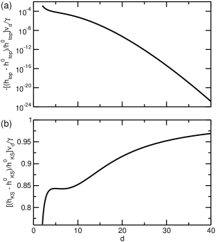
Figure 5: Relative corrections to the topological and to the KS entropy. (a) shows the natural logarithm of $(h_{\rm top}-h^{0}_{\rm top})\nu_{d}/(\gamma h^{0}_{\rm top})$ and (b) shows $(h_{KS}-h^{0}_{KS})\nu_{d}/(\gamma h^{0}_{KS})$, both as functions of $d$, for parameter values $a=1$, $v=1$ and $n=0.001$.

In Fig. 5 the relative corrections to the KS entropy and the topological entropy are plotted as functions of $d$. For $h_{\rm top}$ the ratio to the equilibrium value is very small. It decreases exponentially with $d$, because asymptotically for large $d$ $h^{0}_{top}$ is independent of the radius $a$, whereas the collision frequency $\nu_{d}$ is proportional to $a^{(}d-1)$. For $h_{KS}$ the correction, scaled as in the figure, appoaches unity in the limit of large $d$, as follows readily from eqs. (18) and (6) plus Stirling’s approximation $\ln\Gamma(x)\approx x\ln x-x$.

More dynamical properties can be obtained from $P(\beta)$. The partial Hausdorff dimension is given by the value of $\beta$ where $P(\beta)$ intersects the $\beta$-axis, whereas the partial information dimension is given by the value of $\beta$ where the tangent at $P(1)$ intersects the $\beta$-axis Eckmann and Ruelle (1985); Bohr and Rand (1987). For the latter we easily find that the tangent is given by

$$P(1)-(1-\beta)P^{\prime}(1)$$

$$=(1-\beta)h^{0}_{KS}-k_{0}^{2}\left[D(1)-(1-\beta)D^{\prime}(1)\right].$$ (28)

Thus, the partial information dimension follows as

$$d_{I} = 1-\frac{k_{0}^{2}D(1)}{h^{0}_{KS}+k_{0}^{2}D^{\prime}(1)}$$ (29)

$$= 1-\frac{1}{\frac{1-d}{2}+h^{0}_{KS}(1/\gamma+1/\nu_{d})}$$

and is clearly smaller than unity. For a large system with fixed density an expansion for small escape rates $\gamma$ gives $d_{I}\approx 1-\gamma/h^{0}_{KS}$. The complexity of $P(\beta)$ and the $\beta$-dependence of the diffusion coefficient prevent a calculation of the partial Hausdorff dimension. However, for large systems, where $k_{0}$ is very small, the partial Hausdorff dimension will be very close to $d_{I}$ because the point of intersection of $P(\beta)$ with the $\beta$-axis will be close to $\beta=1$, therefore in Eq. (9) both terms are well approximated by a Taylor expansion around $\beta=1$ up to linear order in $\beta$.

V Discussion

We may conclude first of all that for the Lorentz gas the calculation of corrections to the topological pressure due to open boundary conditions is remarkably simple; it just requires the solution of an effective $\beta$-dependent diffusion equation with the same open boundary conditions. One question that could be asked here is whether the diffusion coefficient to be used in this calculation is the same as in a closed system. Since realizations of the random flight process with a slightly higher than average collision frequency will have a slightly lower diffusion coefficient these will lead to a slightly smaller escape rate from the system. The same can be argued for processes in which the frequency of backscattering events is slightly enhanced and that of forward scattering is slightly suppressed with respect to the averages in an equilibrum system. Therefore the average diffusion coefficient on the repeller should be slightly smaller than the diffusion coefficent of the equilibrium system. However, one easily estimates that the suppression of the diffusion coefficient is of order $k^{2}_{0}$, leading to a correction of order $k_{0}^{4}$ in the escape rate. Our results for the corrections to entropies and dimensions, which are all of order $k_{0}^{2}$, therefore will not be changed. For higher order corrections of course such terms are important.

It is very interesting that for the dilute random Lorentz gas the effects of the open boundary can be separated straightforwardly into effects due to changes in the distributions of free flight times and of scattering angles respectively. This is because the stretching factor first of all factorizes (to leading order in the density) into a product of stretching factors pertaining to a single free flight plus subsequent collision, and in addition each of those factorizes into factors depending on the free flight time respectively the scattering angles alone. Specifically, one has $\Lambda_{d}(\theta,t)=\Lambda_{1}\Lambda_{2}$, with $\Lambda_{1}=(2vt/a)^{d-1}$ and $\Lambda_{2}=\cos^{d-3}\theta$. Rewriting the factor $\Lambda^{1-\beta}$ as $\Lambda_{1}^{1-\beta_{1}}\Lambda_{2}^{1-\beta_{2}}$ one may obtain the topological pressure and the effective diffusion constant as functions of both $\beta_{1}$ and $\beta_{2}$. By taking the derivatives of the topological pressure with respect to $\beta_{1}$ and $\beta_{2}$ one finds that the two terms on the right hand side of Eq. (19) may be assigned to the distributions of free times and of scattering angles respectively. Similarly the correction to the sum of the positive Lyapunov exponents, given by $k^{2}_{0}D^{\prime}(1)$, can be separated into a term due to the change in the free time distribution, which is of the form

$$\Delta_{t}\Sigma\lambda^{+}=k^{2}_{0}D(1)(d-1)\left[\ln\frac{2v}{\nu_{d}a}-{\cal C}-\frac{d-1}{d+1}\right],$$ (30)

and a term due to the change in the distribution of scattering angles, reading

$$\Delta_{\theta}\Sigma\lambda^{+}=k^{2}_{0}\frac{(3-d)}{2}D(1)\left[{\cal C}+\Psi\left(\frac{d+1}{2}\right)-\frac{d-1}{d+1}\right].$$ (31)

One might be tempted to think that the changes in the distribution function are due primarily to particles near the open boundary, which will only survive if their free flights keep them inside the system. This however is completely false. At any given instant the fraction of particles inside a layer of a few mean free paths near the boundary may be estimated as proportional to $1/R^{2}$, with $R$ an estimate for the diameter of the system; the volume fraction covered by the boundary layer is proportional to $1/R$ and the density near the open boundary is also of order $1/R$ compared to the average density. In addition, in order for a particle trajectory to be on the repeller, it has to remain inside the system forever after. For trajectories near the open boundary at the given instant, the probability for this to happen is another order $1/R$ smaller than for trajectories at large van Beijeren et al. (2000). Therefore trajectories getting near the boundary at any time do not contribute at all to the order $k^{2}_{0}$. Rather, the deviations from the equilibrium distributions are caused by the fact that free flights or scattering angles that move a particle away from an open boundary lead to higher survival probability than ones that bring it closer to it. If one wants to know how, locally, the distribution of free times or scattering angles is changed, he would have to take recourse to the methods laid out in Ref. van Beijeren et al. (2000). It is fortunate though, that the reduction of the dynamical partition function to an effective diffusion problem allows one to calculate the KS-entropy and the like, at least up to order $k^{2}_{0}$, without having to go through the details of this formalism.

An interesting question is in how far the present method of calculating corrections to the topological pressure from the solution of a diffusion equation can be generalized to systems of many moving particles. Unfortunately this does not seem to be possible in any straightforward way, even for dilute systems with hard interactions. The reason for this is the semi-dispersing character of the dynamics of these systems, interpreted as billiards in a high dimensional phase space. Due to this property the dynamical partition function does not approximately factorize into a product of terms describing the effects of one free flight and the subsequent collision. Note that even the Lorentz gas loses this property at higher densities, where the mean free path between collisions is not large compared to the scatterer radius.

Finally, we remark that, like in the equilibrium and field driven disordered Lorentz gas, the calculations of the topological pressure for general values of $\beta$ have to be taken with caution Appert et al. (1996); van Beijeren and Dorfman (2002); Mülken and van Beijeren (2004). Points in phase space are weighted by $\Lambda^{1-\beta}$, thus for $\beta$ sufficiently $<1$ the dynamical partition function will be dominated by the largest stretching factors, which are due to trajectories confined to regions of high densities of scatterers. Even though the number of such trajectories decreases exponentially with time, the stretching factors raised to the power $1-\beta$ of the remaining ones will still make these dominant for $\beta$ sufficiently far from 1. For $\beta$ sufficiently $>1$ on the other hand the dynamical partition function will be dominated by trajectories confined to the neighborhood of the least unstable periodic orbit.

In conclusion, we have shown how to relate the thermodynamic formalism for the open Lorentz gas to a diffusive random flight problem. We have calculated the topological pressure in $d$ dimensions as a function of the temperature-like parameter $\beta$. For the open Lorentz gas, the topological pressure is the sum of the topological pressure for the closed system and a $\beta$-dependent effective escape rate which is given by a $\beta$-dependent diffusion coefficient multiplied by the square of the smallest wave number $k_{0}$ fitting the diffusion equation with absorbing boundary equations. From this we have obtained several dynamical quantities such as the Kolmogorov-Sinai entropy, the topological entropy, and the partial information dimension for general dimension $d$.

This work was supported by the Collective and cooperative statistical physics phenomena program of FOM (Fundamenteel Onderzoek der Materie).

References

- Sinai (1972) Y. G. Sinai, Russ. Math. Surv. 27, 21 (1972).
- Ruelle (1978) D. Ruelle, Thermodynamic Formalism (Addison-Wesley Publishing Co., New York, 1978).
- Bowen (1975) R. Bowen, in Lecture Notes in Mathematics (Springer Verlag, Berlin, 1975), vol. 470.
- Eckmann and Ruelle (1985) J.-P. Eckmann and D. Ruelle, Rev. Mod. Phys. 57, 617 (1985).
- Beck and Schlögl (1993) C. Beck and F. Schlögl, Thermodynamics of chaotic systems (Cambridge University Press, New York, 1993).
- Sinai (1970) Y. G. Sinai, Russ. Math. Surv. 25, 137 (1970).
- Hauge (1999) E. H. Hauge, ”What can one learn from Lorentz Models?” in Transport Phenomena edited by G. Kirczenow and J. Marro, Lecture notes in Physics (Springer Verlag, Berlin, 1999), vol. 31, 337.
- Dorfman (1999) J. R. Dorfman, An Introduction to Chaos in Non-Equilibrium Statistical Mechanics (Cambridge University Press, New York, 1999).
- van Beijeren (1982) H. van Beijeren, Rev. Mod. Phys. 54, 195 (1982).
- van Leeuwen and Weijland (1982) J M. J. van Leeuwen, and A. Weyland, Phys. 36, 457 (1967).
- Weyland and van Leeuwen (1982) A. Weyland, and J. M. J. van Leeuwen, Phys. 38, 35 (1968).
- Ernst and Weyland (1982) M. H. Ernst, and A. Weyland, Phys. Lett. A 34, 39 (1971).
- Lorentz (1905) H. A. Lorentz, Proc. Roy. Acad. Amst. 7, 438 (1905).
- van Beijeren and Dorfman (2002) H. van Beijeren and J. R. Dorfman, J. Stat. Phys. 108, 767 (2002).
- van Beijeren et al. (1998) H. van Beijeren, A. Latz, and J. R. Dorfman, Phys. Rev. E 57, 4077 (1998).
- van Beijeren et al. (2000) H. van Beijeren, A. Latz, and J. R. Dorfman, Phys. Rev. E 63, 016312 (2000).
- de Wijn and van Beijeren (2004) A. S. de Wijn and H. van Beijeren, Phys. Rev. E 70, 036209 (2004).
- van Beijeren and Dorfman (1995) H. van Beijeren and J. R. Dorfman, Phys. Rev. Lett. 74, 4412 (1995).
- Mülken and van Beijeren (2004) O. Mülken and H. van Beijeren, Phys. Rev. E 69, 046203 (2004).
- Gradshteyn and Ryzik (1965) I. S. Gradshteyn and I. M. Ryzik, Tables of Integrals, Series, and Products (Academic Press, New York and London, 1965).
- Gaspard and Nicolis (1990) P. Gaspard and G. Nicolis, Phys. Rev. Lett. 65, 1693 (1990).
- Bohr and Rand (1987) T. Bohr and D. Rand, Physica D 25, 387 (1987).
- Appert et al. (1996) C. Appert, H. van Beijeren, M. H. Ernst, and J. R. Dorfman, Phys. Rev. E 54, R1013 (1996).