INTRODUCTION TO CHAOS AND DIFFUSION

I Introduction

This contribution is relative to the opening lectures of the ISSAOS 2001 summer school and it has the aim to provide the reader with some concepts and techniques concerning chaotic dynamics and transport processes in fluids. Our intention is twofold: to give a self-consistent introduction to chaos and diffusion, and to offer a guide for the reading of the rest of this volume.

In the following Section we present some basic elements of the chaotic dynamical systems theory, as the Lyapunov exponents and the Kolmogorov-Sinai entropy. The third Section is devoted to Lagrangian chaos in fluids. The last Section contains an introduction to diffusion and transport processes, with particular emphasis on the treatment of non-ideal cases.

II Some basic elements of dynamical systems

A dynamical system may be defined as a deterministic rule for the time evolution of state observables. Well known examples are the ordinary differential equations (ODE) in which time is continuous:

$${d{\bf x}(t)\over dt}={\bf f}({\bf x}(t)),\;\;\;\;\;{\bf x},{\bf f}\in{\rm I\!R}^{d};$$ (1)

and maps in which time is discrete:

$${\bf x}(t+1)={\bf g}({\bf x}(t)),\;\;\;\;\;{\bf x},{\bf g}\in{\rm I\!R}^{d}.$$ (2)

In the case of maps, the evolution law is straightforward: from ${\bf x}(0)$ one computes ${\bf x}(1)$, and then ${\bf x}(2)$ and so on. For ODE’s, under rather general assumptions on f, from an initial condition ${\bf x}(0)$ one has a unique trajectory ${\bf x}(t)$ for $t>0$ [47]. Examples of regular behaviors (e.g. stable fixed points, limit cycles) are well known, see Figure 1.

FIG. 1.: Examples of regular attractors: fixed point (above) and limit cycle (below).

A rather natural question is the possible existence of less regular behaviors i.e. different from stable fixed points, periodic or quasi-periodic motion.

After the seminal works of Poincaré, Lorenz and Hénon (to cite only the most eminent ones) it is now well established that the so called chaotic behavior is ubiquitous. As a relevant system, originated in the geophysical context, we mention the celebrated Lorenz model [40]:

$${dx\over dt} = -\sigma(x-y)$$ (3)

$${dy\over dt} = -xz+rx-y$$ (4)

$${dz\over dt} = xy-bz$$ (5)

This system is related to the Rayleigh-Benard convection under very crude approximations. The quantity $x$ is proportional the circulatory fluid particle velocity; the quantities $y$ and $z$ are related to the temperature profile; $\sigma$, $b$ and $r$ are dimensionless parameters. Lorenz studied the case with $\sigma=10$ and $b=8/3$ at varying $r$ (which is proportional to the Rayleigh number). It is easy to see by linear analysis that the fixed point $(0,0,0)$ is stable for $r<1$. For $r>1$ it becomes unstable and two new fixed points appear:

$$C_{+,-}=(\pm\sqrt{b(r-1)},\pm\sqrt{b(r-1)},r-1),$$ (6)

these are stable for $r<r_{c}=24.74$. A nontrivial behavior, i.e. non periodic, is present for $r>r_{c}$, as is shown in Figure 2.

In this “strange”, chaotic regime one has the so called sensitive dependence on initial conditions. Consider two trajectories, ${\bf x}(t)$ and ${\bf x}^{\prime}(t)$, initially very close and denote with $\Delta(t)=||{\bf x}^{\prime}(t)-{\bf x}(t)||$ their separation. Chaotic behavior means that if $\Delta(0)\to 0$, then as $t\to\infty$ one has $\Delta(t)\sim\Delta(0)\exp{\lambda_{1}t}$, with $\lambda_{1}>0$, see Figure 3.

Let us notice that, because of its chaotic behavior and its dissipative nature, i.e.

$${\partial\dot{x}\over\partial x}+{\partial\dot{y}\over\partial y}+{\partial\dot{z}\over\partial z}<0,$$ (7)

the attractor of the Lorenz system cannot be a smooth surface. Indeed the attractor has a self-similar structure with a fractal dimension between $2$ and $3$. The Lorenz model (which had an important historical relevance in the development of chaos theory) is now considered a paradigmatic example of a chaotic system.

FIG. 2.: Example of aperiodic signal: the $x$ variable of the Lorenz system (4) as function of time $t$, for $r=28$.

FIG. 3.: The growth of a generic infinitesimal perturbation $\Delta(t)$ in the Lorenz model (4) as function of time $t$, for $r=28$. The dashed line represent the exponential growth $\Delta(0)\exp{\lambda_{1}t}$.

A Lyapunov exponents

The sensitive dependence on the initial conditions can be formalized in order to give it a quantitative characterization. The main growth rate of trajectory separation is measured by the first (or maximum) Lyapunov exponent, defined as

$$\lambda_{1}=\lim_{t\to\infty}\lim_{\Delta(0)\to 0}{1\over t}\ln{\Delta(t)\over\Delta(0)},$$ (8)

As long as $\Delta(t)$ remains sufficiently small (i.e. infinitesimal, strictly speaking), one can regard the separation as a tangent vector ${\bf z}(t)$ whose time evolution is

$${dz_{i}\over dt}=\sum_{j=1}^{d}{\partial f_{i}\over\partial x_{j}}|_{{\bf x}(t)}\cdot z_{j},$$ (9)

and, therefore,

$$\lambda_{1}=\lim_{t\to\infty}{1\over t}\ln{||{\bf z}(t)||\over||{\bf z}(0)||}.$$ (10)

In principle, $\lambda_{1}$ may depend on the initial condition ${\bf x}(0)$, but this dependence disappears for ergodic systems. In general there exist as many Lyapunov exponents, conventionally written in decreasing order $\lambda_{1}\geq\lambda_{2}\geq\lambda_{3}\geq...$, as the independent coordinates of the phase space [8]. Without entering the details, one can define the sum of the first $k$ Lyapunov exponents as the growth rate of an infinitesimal $k-$dimensional volume in the phase space. In particular, $\lambda_{1}$ is the growth rate of material lines, $\lambda_{1}+\lambda_{2}$ is the growth rate of $2D$ surfaces, and so on. A numerical widely used efficient method is due to Benettin et al. [8].

It must be observed that, after a transient, the growth rate of any generic small perturbation (i.e. distance between two initially close trajectories) is measured by the first (maximum) Lyapunov exponent $\lambda_{1}$, and $\lambda_{1}>0$ means chaos. In such a case, the state of the system is unpredictable on long times. Indeed, if we want to predict the state with a certain tolerance $\Delta$ then our forecast cannot be pushed over a certain time interval $T_{P}$, called predictability time, given by:

$$T_{P}\sim{1\over\lambda_{1}}\ln{\Delta\over\Delta(0)}.$$ (11)

The above relation shows that $T_{P}$ is basically determined by $1/\lambda_{1}$, seen its weak dependence on the ratio $\Delta/\Delta(0)$. To be precise one must state that, for a series of reasons, relation (11) is too simple to be of actual relevance [14].

B The Kolmogorov-S entropy

Deterministic chaotic systems, because of their irregular behavior, have many aspects in common with stochastic processes. The idea of using stochastic processes to mimic chaotic behavior, therefore, is rather natural [21, 9]. One of the most relevant and successful approaches is symbolic dynamics [7]. For the sake of simplicity let us consider a discrete time dynamical system. One can introduce a partition ${\cal A}$ of the phase space formed by N disjoint sets $A_{1},...,A_{N}$. From any initial condition one has a trajectory

$${\bf x}(0)\to{\bf x}(1),{\bf x}(2),...,{\bf x}(n),...$$ (12)

dependently on the partition element visited, the trajectory (12), is associated to a symbolic sequence

$${\bf x}(0)\to i_{1},i_{2},...,i_{n},...$$ (13)

where $i_{n}$ ($i_{n}\in(1,2,...,N)$) means that ${\bf x}(n)\in A_{i_{n}}$ at the step $n$, for $n=1,2,...$. The coarse-grained properties of chaotic trajectories are therefore studied through the discrete time process (13).

An important characterization of symbolic dynamics is given by the Kolmogorov-Sinai (K-S) entropy, defined as follows. Let $C_{n}=(i_{1},i_{2},...,i_{n})$ be a generic “word” of size $n$ and $P(C_{n})$ its occurrence probability, the quantity

$$H_{n}=\sup_{A}[-\sum_{C_{n}}P(C_{n})\ln P(C_{n})]$$ (14)

is called block entropy of the $n$-sequences, and it is computed by taking the largest value over all possible partitions. In the limit of infinitely long sequences, the asymptotic entropy increment

$$h_{KS}=\lim_{n\to\infty}H_{n+1}-H_{n}$$ (15)

is called Kolmogorov-Sinai entropy. The difference $H_{n+1}-H_{n}$ has the intuitive meaning of average information gain supplied by the $(n+1)-$th symbol, provided that the previous $n$ symbols are known. K-S entropy has an important connection with the positive Lyapunov exponents of the system [47]:

$$h_{KS}=\sum_{\lambda_{i}>0}\lambda_{i}$$ (16)

In particular, for low-dimensional chaotic systems for which only one Lyapunov exponent is positive, one has $h_{KS}=\lambda_{1}$.

We observe that in (14) there is a technical difficulty, i.e. taking the sup over all the possible partitions. However, sometimes there exits a special partition, called generating partition, for which one finds that $H_{n}$ coincides with its superior bound. Unfortunately the generating partition is often hard to find, even admitting that it exist. Nevertheless, given a certain partition, chosen by physical intuition, the statistical properties of the related symbol sequences can give information on the dynamical system beneath. For example, if the probability of observing a symbol (state) depends only by the knowledge of the immediately preceding symbol, the symbolic process is called a Markov chain and all the statistical properties are determined by the transition matrix elements $W_{ij}$ giving the probability of observing a transition $i\to j$ in one time step. If the memory of the system extends far beyond the time step between two consecutive symbols, and the occurrence probability of a symbol depends on $k$ preceding steps, the process is called Markov process of order $k$ and, in principle, a $k$ rank tensor would be required to describe the dynamical system with good accuracy. It is possible to demonstrate that if $H_{n+1}-H_{n}=h_{KS}$ for $n\geq k+1$, $k$ is the (minimum) order of the required Markov process [32]. It has to be pointed out, however, that to know the order of the suitable Markov process we need is of no practical utility if $k\gg 1$.

For applications of the Markovian approach to geophysical systems see [19] and the contributions by Abel et al. and by Pasmanter et al. in this volume.

III Lagrangian Chaos

A problem of great interest concerns the study of the spatial and temporal structure of the so-called passive fields, indicating by this term passively quantities driven by the flow, such as the temperature under certain conditions [45]. The equation for the evolution of a passive scalar field $\theta({\bf x},t)$, advected by a velocity field ${\bf v}({\bf x},t)$, is

$$\partial_{t}\theta+\nabla\cdot({\bf v}\,\theta)=\chi\,\nabla^{2}\theta$$ (17)

where ${\bf v}({\bf x},t)$ is a given velocity field and $\chi$ is the molecular diffusion coefficient.

The problem (17) can be studied through two different approaches. Either one deals at any time with the field $\theta$ in the space domain covered by the fluid, or one deals with the trajectory of each fluid particle. The two approaches are usually designed as “Eulerian”and “Lagrangian”, although both of them are due to Euler [34]. The two points of view are in principle equivalent.

The motion of a fluid particle is determined by the differential equation

$${d{\bf x}\over dt}={\bf v}({\bf x},t)$$ (18)

which also describes the motion of test particles, for example a powder embedded in the fluid, provided that the particles are neutral and small enough not to perturb the velocity field, although large enough not to perform a Brownian motion. Particles of this type are commonly used for flow visualization in fluid mechanics experiments, see [51] and the contribution of Cenedese et al. in this volume. Let us note that the true equation for the motion of a material particle in a fluid can be rather complicated [43, 22].

It is now well established that even in regular velocity field the motion of fluid particles can be very irregular [29, 2]. In this case initially nearby trajectories diverge exponentially and one speaks of Lagrangian chaos. In general, chaotic behaviors can arise in two-dimensional flow only for time dependent velocity fields in two dimensions, while it can be present even for stationary velocity fields in three dimensions.

If $\chi=0$, it is easy to realize that (17) is equivalent to (18). In fact, we can write

$$\theta({\bf x},t)=\theta_{o}({T}^{-t}{\bf x})$$ (19)

where $\theta_{o}({\bf x})=\theta({\bf x},t=0)$ and ${T}$ is the formal evolution operator of (18) ,

$${\bf x}(t)={T}^{t}{\bf x}(0).$$ (20)

Taking into account the molecular diffusion $\chi$, (17) is the Fokker-Planck equation of the Langevin equation [20]

$${d{\bf x}\over dt}={\bf v}({\bf x},t)+{\eta}(t)$$ (21)

where ${\eta}$ is a Gaussian process with zero mean and variance

$$\left\langle{\eta_{i}(t)\,\eta_{j}(t^{\prime})}\right\rangle=2\chi\delta_{ij}\,\delta(t-t^{\prime}).$$ (22)

In the following we will consider only incompressible flow

$$\nabla\cdot{\bf v}=0$$ (23)

for which the dynamical system (18) is conservative. In two dimensions, the constraint (23) is automatically satisfied assuming

$$v_{1}={\partial\psi\over\partial x_{2}},\qquad v_{2}=-\,{\partial\psi\over\partial x_{1}}$$ (24)

where $\psi({\bf x},t)$ is the stream function. Inserting (24) into (18) the evolution equations become

$${{dx_{1}}\over{dt}}={\partial\psi\over\partial x_{2}},\qquad{{dx_{2}}\over{dt}}=-\,{\partial\psi\over\partial x_{1}}.$$ (25)

Formally (25) is a Hamiltonian system with the Hamiltonian given by the stream function $\psi$.

A Examples of Lagrangian chaos

As a first example we consider a $3d$ stationary velocity field, the so-called ABC flow

$${\bf v}=\left(A\sin z+C\cos y,\,B\sin x+A\cos z,\,C\sin y+B\cos x\right)$$ (26)

where $A,\,B$ and $C$ are non zero real parameters. Because of the incompressibility condition, the evolution ${\bf x}(0)\to{\bf x}(t)$ defines a volume preserving, dynamics.

Arnold [4] argued that (26) is a good candidate for chaotic motion. Let us briefly repeat his elegant argument. For a steady state solution of the $3d$ Euler equation one has:

$$\nabla\cdot{\bf v} = 0$$ (27)

$${\bf v}\times(\nabla\times{\bf v}) = \nabla\alpha$$ (28)

$$\alpha = {P\over\rho}+{{\bf v}^{2}\over 2}$$ (29)

where $P$ is the pressure and $\rho$ the density. As a consequence of the Bernoulli theorem [35], $\alpha({\bf x})$ is constant along a streamline – that is a Lagrangian trajectory ${\bf x}(t)$. One can easily verify that chaotic motion can appear only if $\alpha({\bf x})$ is constant (i.e. $\nabla\alpha({\bf x})=0$) in a part of the space. Otherwise the trajectory would be confined on a $2d$ surface $\alpha({\bf x})=$ constant, where the motion must be regular as a consequence of general arguments [47]. In order to satisfy such a constraint, from (28) one has the Beltrami condition:

$$\nabla\times{\bf v}=\gamma({\bf x})\,{\bf v}.$$ (30)

The reader can easily verify that the field ${\bf v}$ given by (26) satisfy (30) (in this case $\gamma({\bf x})=$ constant). Indeed, numerical experiments by Hénon [29] provided evidence that Lagrangian motion under velocity (26) is chaotic for typical values of the parameters $A$, $B$, and $C$ (see an example in Figure 4).

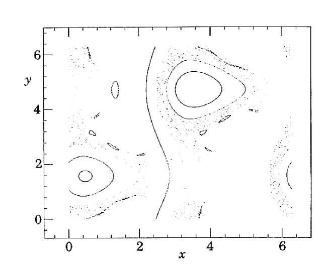
FIG. 4.: Intersections with the Poincaré section, plane $z=0$, of eight trajectories of the ABC flow with parameters $A=2.0$, $B=1.70$, $C=1.50$.

In a two-dimensional incompressible stationary flows the motion of fluid particles is given by a time independent Hamiltonian system with one degree of freedom and, since trajectories follow iso-$\psi$ lines, it is impossible to have chaos. However, for explicit time dependent stream function $\psi$ the system (26) can exhibit chaotic motion [47].

In the particular case of time periodic velocity fields, ${\bf v}({\bf x},t+T)={\bf v}({\bf x},t)$, the trajectory of (18) can be studied in terms of discrete dynamical systems: the position ${\bf x}(t+T)$ is determined in terms of ${\bf x}(t)$. The map ${\bf x}(t)\to{\bf x}(t+T)$ will not depend on $t$ thus (18) can be written in the form

$${\bf x}(n+1)={\bf F}[{\bf x}(n)],$$ (31)

where now the time is measured in units of the period $T$. Because of incompressibility, the map (31) is conservative:

$$\bigl{|}\det{A}[{\bf x}]\bigr{|}=1,\qquad{\rm where}\qquad A_{ij}[{\bf x}]={\partial F_{i}[{\bf x}]\over\partial x_{j}}.$$ (32)

An explicit deduction of the form of ${\bf F}$ for a general $2d$ or $3d$ flow is usually very difficult. However, in some simple model of can be deduced on the basis of physical features [3, 18].

B Eulerian properties and Lagrangian chaos

In principle, the evolution of the velocity field ${\bf v}$ is described by partial differential equations, e.g. Navier-Stokes or Boussinesq equations. However, often in weakly turbulent situations, a good approximation of the flow can be obtained by using a Galerkin approach, and reducing the Eulerian problem to a (small) system of $F$ ordinary differential equations [15, 37]. The motion of a fluid particle is then described by the $(d+F)$-dimensional dynamical system

$${d{\bf Q}\over dt}={\bf f}({\bf Q},t)\qquad\hbox{\rm with}\ {\bf Q},\,{\bf f}\,\in{\rm I\!R}^{F}$$ (33)

$${d{\bf x}\over dt}={\bf v}({\bf x},{\bf Q})\qquad\hbox{\rm with}\ {\bf x},\,{\bf v}\in{\rm I\!R}^{d}$$ (34)

where $d$ is the space dimensionality and ${\bf Q}=(Q_{1},...Q_{F})$ are the $F$ variables, usually normal modes, which are a representation of the velocity field ${\bf v}$. Note that the Eulerian equations (33) do not depend on the Lagrangian part (34) and can be solved independently.

In order to characterize the degree of chaos, three different Lyapunov exponents can be defined [25]:

• a) $\lambda_{\rm E}$ for the Eulerian part (33);

• b) $\lambda_{\rm L}$ for the Lagrangian part (34), where the evolution of the velocity field is assumed to be known;

• c) $\lambda_{\rm T}$ per for the total system of the $d+F$ equations.

These Lyapunov exponents are defined as:

$$\lambda_{\rm E,L,T}=\lim_{t\to\infty}\,{1\over t}\,\ln{|{\bf z}(t)^{({\rm E,L,T})}|\over|{\bf z}(0)^{({\rm E,L,T})}|}$$ (35)

where the evolution of the three tangent vectors ${\bf z}$ are given by the linearized stability equations for the Eulerian part, for the Lagrangian part and for the total system, respectively:

$${dz_{i}^{({\rm E})}\over dt}=\sum_{j=1}^{F}\left.{\partial f_{i}\over\partial Q_{j}}\right|_{{\bf Q}(t)}\,{z_{j}}^{({\rm E})},\qquad{\bf z}^{({\rm E})}\,\in{\rm I\!R}^{F}$$ (36)

$${dz_{i}^{({\rm L})}\over dt}=\sum_{j=1}^{d}\left.{\partial v_{i}\over\partial x_{j}}\right|_{{\bf x}(t)}\,{z_{j}}^{({\rm L})},\qquad{\bf z}^{({\rm L})}\,\in{\rm I\!R}^{d}$$ (37)

$${dz_{i}^{({\rm T})}\over dt}=\sum_{j=1}^{d+F}\left.{\partial G_{i}\over\partial y_{j}}\right|_{{\bf y}(t)}\,{z_{j}}^{({\rm T})},\qquad{\bf z}^{({\rm T})}\,\in{\rm I\!R}^{F+d}$$ (38)

and ${\bf y}=(Q_{1},\ldots,Q_{F},x_{1},\ldots,x_{d})$ and ${\bf G}=(f_{1},\ldots,f_{F},v_{1},\ldots,v_{d})$. The meaning of these Lyapunov exponents is evident:

• a) $\lambda_{\rm E}$ is the mean exponential rate of the increasing of the uncertainty in the knowledge of the velocity field (which is, by definition, independent on the Lagrangian motion);

• b) $\lambda_{\rm L}$ estimates the rate at which the distance $\delta x(t)$ between two fluid particles initially close increases with time, when the velocity field is given, i.e. a particle pair in the same Eulerian realization;

• c) $\lambda_{\rm T}$ is the rate of growth of the distance between initially close particle pairs, when the velocity field is not known with infinite precision.

There is no general relation between $\lambda_{\rm E}$ and $\lambda_{\rm L}$. One could expect that in presence of a chaotic velocity field the particle motion has to be chaotic. However, the inequality $\lambda_{\rm L}\geq\lambda_{\rm E}$ – even if generic – sometimes does not hold, e.g. in some systems like the Lorenz model [25] and in generic $2d$ flows when the Lagrangian motion happens around well defined vortex structures [6] as discussed in the following. On the contrary, one has [23]

$$\lambda_{\rm T}={\rm max}\,(\lambda_{\rm E},\lambda_{\rm L}).$$ (39)

C Lagrangian chaos in two dimensional flows

Let us now consider the two–dimensional Navier-Stokes equations with periodic boundary conditions at low Reynolds numbers, for which we can expand the stream function $\psi$ in Fourier series and takes into account only the first $F$ terms [15, 37],

$$\psi=-i\sum_{j=1}^{F}\ k_{j}^{-1}Q_{{}_{j}}e^{i{\bf k}_{j}{\bf x}}+{\rm c.c.}\,,$$ (40)

where c.c. indicates the complex conjugate term and ${\bf Q}=(Q_{1},\ldots,Q_{F})$ are the Fourier coefficients. Inserting (40) into the Navier-Stokes equations and by an appropriate time rescaling, we obtain the system of $F$ ordinary differential equations

$${dQ_{j}\over dt}=-k_{j}^{2}\,Q_{j}+\sum_{l,m}A_{jlm}Q_{l}Q_{m}+f_{j},$$ (41)

in which $f_{j}$ represents an external forcing.

Franceschini and coworkers have studied this truncated model with $F=5$ and $F=7$ [15, 37]. The forcing were restricted to the $3^{th}$ mode $f_{j}={\rm Re}\,\delta_{j,3}$ [37]. For $F=5$ and ${\rm Re}<{\rm Re}_{1}=22.85\ldots$, there are four stable stationary solutions, say $\widehat{\bf Q}$, and $\lambda_{\rm E}<0$. At ${\rm Re}={\rm Re}_{1}$, these solutions become unstable, via a Hopf bifurcation [42], and four stable periodic orbits appear, still implying $\lambda_{\rm E}=0$. For ${\rm Re}_{1}<{\rm Re}<{\rm Re}_{2}=28.41\ldots$, one thus finds the stable limit cycles:

$${\bf Q}(t)=\widehat{\bf Q}+({\rm Re}-{\rm Re}_{1})^{1/2}\delta{\bf Q}(t)+O({\rm Re}-{\rm Re}_{1})$$ (42)

where $\delta{\bf Q}(t)$ is periodic with period

$$T({\rm Re})=T_{0}+O({\rm Re}-{\rm Re}_{1})\qquad T_{0}=0.7328\ldots$$ (43)

At ${\rm Re}={\rm Re}_{2}$, these limit cycles lose stability and there is a period doubling cascade toward Eulerian chaos.

Let us now discuss the Lagrangian behavior of a fluid particle. For ${\rm Re}<{\rm Re}_{1}$, the stream function is asymptotically stationary, $\psi({\bf x},t)\to\widehat{\psi}({\bf x})$, and the corresponding one-dimensional Hamiltonian is time-independent, therefore Lagrangian trajectories are regular. For ${\rm Re}={\rm Re}_{1}+\epsilon$ the stream function becomes time dependent

$$\psi({\bf x},t)=\widehat{\psi}({\bf x})+\sqrt{\epsilon}\,\delta\psi({\bf x},t)+O(\epsilon),$$ (44)

where $\widehat{\psi}({\bf x})$ is given by $\widehat{{\bf Q}}$ and $\delta\psi$ is periodic in ${\bf x}$ and in $t$ with period $T$. The region of phase space, here the real two-dimensional space, adjacent to a separatrix is very sensitive to perturbations, even of very weak intensity. Figure 5 shows the structure of the separatrices, i.e. the orbits of infinite periods at ${\rm Re}={\rm Re}_{1}-0.05$.

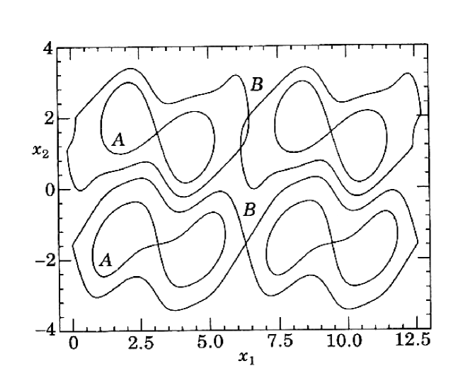
FIG. 5.: Structure of the separatrices in the 5-mode model (40) with ${\rm Re}={\rm Re}_{1}-0.05$.

Indeed, generically in one-dimensional Hamiltonian systems, a periodic perturbation gives origin to stochastic layers around the separatrices where the motion is chaotic, as consequence of unfolding and crossing of the stable and unstable manifolds in domains centered at the hyperbolic fixed points [21, 47]. One has strong numerical evidence for the existence of the chaotic regions, see Figure 6.

Chaotic and regular motion for small $\epsilon={\rm Re}_{1}-{\rm Re}$ can be studied by the Poincaré map

$${\bf x}(nT)\to{\bf x}(nT+T).$$ (45)

The period $T(\epsilon)$ is computed numerically. The size of the stochastic layers rapidly increase with $\epsilon$. At $\epsilon=\epsilon_{\rm c}\approx 0.7$ they overlap and it is practically impossible to distinguish between regular and chaotic zones. At $\epsilon>\epsilon_{\rm c}$ there is always diffusive motion.

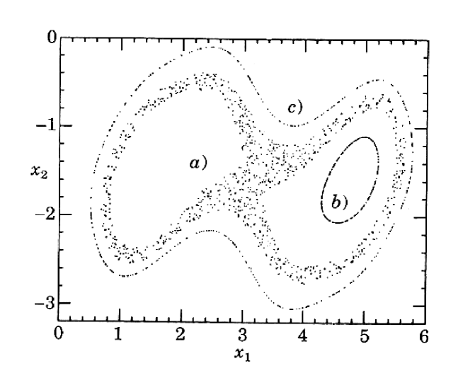
FIG. 6.: Poincaré map for three trajectories of the 5-mode model with ${\rm Re}={\rm Re}_{1}+0.05$. The initial conditions are selected close to a separatrix, case a) ($x_{1}(0)=3.2$, $x_{2}(0)=-1.6$), or far from the separatrices, cases b) ($x_{1}(0)=4.3$, $x_{2}(0)=-2.0$) and c) ($x_{1}(0)=4.267$, $x_{2}(0)=-3.009$).

We stress that this scenario for the onset of Lagrangian chaos in two-dimensional fluids is generic and does not depend on the particular truncated model. In fact, it is only related to the appearance of stochastic layers under the effects of small time-dependent perturbations in one-dimensional integrable Hamiltonian systems. As consequence of a general features of one-dimensional Hamiltonian systems we expect that a stationary stream function becomes time periodic through a Hopf bifurcation as occurs for all known truncated models of Navier-Stokes equations.

We have seen that there is no simple relation between Eulerian and Lagrangian behaviors. In the following, we shall discuss two important points:

• (i) what are the effects on the Lagrangian chaos of the transition to Eulerian chaos, i.e. from $\lambda_{\rm E}=0$ to $\lambda_{\rm E}>0$.

• (ii) whether a chaotic velocity field ($\lambda_{\rm E}>0$) always implies an erratic motion of fluid particles.

The first point can be studied again within the $F=5$ modes model (41). Increasing ${\rm Re}$, the limit cycles bifurcate to new double period orbits followed by a period doubling transition to chaos and a strange attractor appears at ${\rm Re}_{c}\approx 28.73$, where $\lambda_{\rm E}$ becomes positive. These transitions have no signature on Lagrangian behavior, as it is shown in Figure 7, i.e. the onset of Eulerian chaos has no influence on Lagrangian properties.

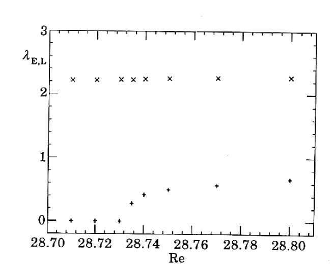
FIG. 7.: Lyapunov exponents $\lambda_{E}$ ($+$) and $\lambda_{L}$ ($\times$) as function of ${\rm Re}$ around ${\rm Re}_{c}$, for the 5-mode model.

This feature should be valid in most situations, since it is natural to expect that in generic cases there is a strong separation of the characteristic times for Eulerian and Lagrangian behaviors.

The second point – the conjecture that a chaotic velocity field always implies chaotic motion of particles – looks very reasonable. Indeed, it appears to hold in many systems [23]. Nevertheless, one can find a class of systems where it is false, e.g. the equations (33), (34) may exhibit Eulerian chaoticity $\lambda_{\rm E}>0$, even if $\lambda_{\rm L}=0$ [6].

Consider for example the motion of $N$ point vortices in the plane with circulations $\Gamma_{i}$ and positions $(x_{i}(t),y_{i}(t))$ ($i=1,..N$) [1]:

$$\Gamma_{i}{{dx_{i}}\over{dt}}={{\partial H}\over{\partial y_{i}}}$$ (46)

$$\Gamma_{i}{{dy_{i}}\over{dt}}=-{{\partial H}\over{\partial x_{i}}}$$ (47)

where

$$H=-{1\over{4\pi}}\sum_{i\neq j}\Gamma_{i}\Gamma_{j}\ln r_{ij}$$ (48)

and $r_{ij}^{2}=(x_{i}-x_{j})^{2}+(y_{i}-y_{j})^{2}$.

The motion of $N$ point vortices is described in an Eulerian phase space with $2N$ dimensions. Because of the presence of global conserved quantities, a system of three vortices is integrable and there is no exponential divergence of nearby trajectories in phase space. For $N\geq 4$, apart from non generic initial conditions and/or values of the parameters $\Gamma_{i}$, the system is chaotic [1].

The motion of a passively advected particle located in $(x(t),y(t))$ in the velocity field defined by (46-47) is given

$${{dx}\over{dt}}=-\sum_{i}{{\Gamma_{i}}\over{2\pi}}{{y-y_{i}}\over{R_{i}^{2}}}$$ (49)

$${{dy}\over{dt}}=\sum_{i}{{\Gamma_{i}}\over{2\pi}}{{x-x_{i}}\over{R_{i}^{2}}}$$ (50)

where $R_{i}^{2}=(x-x_{i})^{2}+(y-y_{i})^{2}$.

Let us first consider the motion of advected particles in a three-vortices (integrable) system in which $\lambda_{E}=0$. In this case, the stream function for the advected particle is periodic in time and the expectation is that the advected particles may display chaotic behavior. The typical trajectories of passive particles which have initially been placed respectively in close proximity of a vortex center or in the background field between the vortices display a very different behavior. The particle seeded close to the vortex center displays a regular motion around the vortex and thus $\lambda_{L}=0$; by contrast, the particle in the background field undergoes an irregular and aperiodic trajectory, and $\lambda_{L}$ is positive.

We now discuss a case where the Eulerian flow is chaotic i.e. $N=4$ point vortices. Let us consider again the trajectory of a passive particle deployed in proximity of a vortex center. As before, the particle rotates around the moving vortex. The vortex motion is chaotic; consequently, the particle position is unpredictable on large times as is the vortex position. Nevertheless, the Lagrangian Lyapunov exponent for this trajectory is zero (i.e. two initially close particles around the vortex remain close), even if the Eulerian Lyapunov exponent is positive, see Figure 8.

,,,

FIG. 8.: Particle trajectories in the four-vortex system. Eulerian dynamics in this case is chaotic. The left panel shows a regular Lagrangian trajectory while the right panel shows a chaotic Lagrangian trajectory. The different behavior of the two particles is due to different initial conditions.

This result indicates once more that there is no strict link between Eulerian and Lagrangian chaoticity.

One may wonder whether a much more complex Eulerian flow, such as $2d$ turbulence, may give the same scenario for particle advection: i.e. regular trajectories close to the vortices and chaotic behavior between the vortices. It has been shown that this is indeed the case [6] and that the chaotic nature of the trajectories of advected particles is not strictly determined by the complex time evolution of the turbulent flow.

We have seen that there is no general relation between Lagrangian and Eulerian chaos. In the typical situation Lagrangian chaos may appear also for regular velocity fields. However, it is also possible to have the opposite situation, with $\lambda_{\rm L}=0$ in presence of Eulerian chaos, as in the example of Lagrangian motion inside vortex structures. As an important consequence of this discussion we remark that it is not possible to separate Lagrangian and Eulerian properties in a measured trajectory, e.g. a buoy in the oceanic currents [46]. Indeed, using the standard methods for data analysis [27], from Lagrangian trajectories one extracts the total Lyapunov exponent $\lambda_{\rm T}$ and not $\lambda_{\rm L}$ or $\lambda_{\rm E}$.

IV Transport and diffusion

The simplest model of diffusion is the Brownian motion, the erratic movement of a grains suspended in liquid observed by the botanist Robert Brown as early as in 1827. After the fundamental work of Einstein [24] and Langevin [36], Brownian motion become the prototypical example of stochastic process.

A The random walk model for Brownian motion

In order to study more in detail the properties of diffusion, let us introduce the simplest model of Brownian motion, i.e. the one-dimensional random walk. The walker moves on a line making discrete jumps $v_{i}=\pm 1$ at discrete times. The position of the walker, started at the origin at $t=0$, will be

$$R(t)=\sum_{i=1}^{t}v_{i}$$ (51)

Assuming equiprobability for left and right jumps (no mean motion), the probability that at time $t$ the walker is in position $x$ will be

$$p_{t}(R=x)=prob\left[\begin{array}[]{c}{t-x\over 2}steps-1\\ {t+x\over 2}steps+1\end{array}\right]={1\over 2^{t}}\left(\begin{array}[]{c}t\\ {t+x\over 2}\end{array}\right)$$ (52)

For large $t$ and $x$ (i.e. after many microscopic steps) we can use Stirling approximation and get

$$p_{t}(x)=\sqrt{{t\over 2\pi(t^{2}-x^{2})}}\exp{\left[-{t+x\over 2}\ln{t+x\over 2}-{t-x\over 2}\ln{t-x\over 2}\right]}$$ (53)

The core of the distribution recovers the well known Gaussian form, i.e. for $x\ll t$ from (53) we get

$$p_{t}(x)=\sqrt{{1\over 2\pi t}}\exp\left(-{x^{2}\over 2t}\right)$$ (54)

From (54) one obtains that the variance of the displacement follows diffusive behavior, i.e.

$$\langle x^{2}(t)\rangle=2t$$ (55)

We stress that diffusion is obtained only asymptotically (i.e. for $t\to\infty$). This is a consequence of central limit theorem which assures Gaussian distributions and diffusive behavior in the limit of many independent jumps. The necessary, and sufficient, condition for observing diffusive regime is the existence of a finite correlation time (here represented by discrete time between jumps) for the microscopic dynamics. Let us stress that this is the important ingredient for diffusion, and not a stochastic microscopic dynamics. We will see below that diffusion can arise even in completely deterministic systems.

Another important remark is that Gaussian distribution (54) is intrinsic of diffusion process, independent on the distribution of microscopic jumps: indeed only the first two moments of $v_{i}$ enter into expression (54). This is, of course, the essence of the central limit theorem. Following the above derivation, it is clear that this is true only in the core of the distribution. The far tails keep memory of the microscopic process and are, in general, not Gaussian. As an example, in Figure 9 we plot the pdf $p_{t}(x)$ at step $t=100$ compared with the Gaussian approximation. Deviations are evident in the tails.

FIG. 9.: Probability distribution function of the one-dimensional random walk after $t=100$ steps. The dashed line is the Gaussian distribution

The Gaussian distribution (54) can be obtained as the solution of the diffusion equation which governs the evolution of the probability in time. This is the Fokker-Planck equation for the particular stochastic process. A direct way to relate the one-dimensional random walk to the diffusion equation is obtained by introducing the master equation, i.e. the time evolution of the probability [26]:

$$p_{t+1}(x)={1\over 2}p_{t}(x-1)+{1\over 2}p_{t}(x+1)\,.$$ (56)

In order to get a continuous limit, we introduce explicitly the steps $\Delta x$ and $\Delta t$ and write

$${p_{t+\Delta t}(x)-p_{t}(x)\over\Delta t}={(\Delta x)^{2}\over 2\Delta t}{p_{t}(x+\Delta x)+p_{t}(x-\Delta x)-2p_{t}(x)\over(\Delta x)^{2}}\,.$$ (57)

Now, taking the limit $\Delta x,\Delta t\to 0$ in such a way that $(\Delta x)^{2}/\Delta t\to 2D$ (the factor $2$ is purely conventional) we obtain the diffusion equation

$${\partial p(x,t)\over\partial t}=D{\partial^{2}p(x,t)\over\partial x^{2}}\,.$$ (58)

The way the limit $\Delta x,\Delta t\to 0$ is taken reflects the scaling invariance property of diffusion equation. The solution to (58) is readily obtained as

$$p(x,t)={1\over\sqrt{4\pi Dt}}\exp\left(-{x^{2}\over 4Dt}\right)\,.$$ (59)

Diffusion equation (58) is here written for the probability $p(x,t)$ of observing a marked particle (a tracer) in position $x$ at time $t$. The same equation can have another interpretation, in which $p(x,t)=\theta(x,t)$ represents the concentration of a scalar quantity (marked fluid, temperature, pollutant) as function of time. The only difference is, of course, in the normalization.

B Less simple transport processes

As already stated time decorrelation is the key ingredient for diffusion. In the random walker model it is a consequence of randomness: the steps $v_{i}$ are random uncorrelated variables and this assures the applicability of central limit theorem. But we can have a finite time correlation and thus diffusion also without randomness. To be more specific, let us consider the following deterministic model (standard map [21]):

$$\left\{\begin{array}[]{ccc}J(t+1)&=&J(t)+K\sin\theta(t)\\ \theta(t+1)&=&\theta(t)+J(t+1)\end{array}\right.$$ (60)

FIG. 10.: Square dispersion $\langle J(t)^{2}\rangle$ for the standard map at $K=10.5$. The dashed line is the RPA prediction.

The map is known to display large-scale chaotic behavior for $K>K_{c}\simeq 0.9716$ and, as a consequence of deterministic chaos, $J(t)$ has diffusive behavior. For large times, $J(t)$ is large and thus the angle $\theta(t)$ rotates rapidly. In this limit, we can assume that at each step $\theta(t)$ decorrelates and thus write

$$J(t)^{2}=K^{2}\left(\sum_{t^{\prime}=1}^{t}\sin\theta(t^{\prime})\right)^{2}\simeq K^{2}\langle\sin^{2}\theta\rangle t=2Dt$$ (61)

The diffusion coefficient $D$, in the random phase approximation, i.e. assuming that $sin\theta(t)$ is not correlated with $sin\theta(t^{\prime})$ for $t\neq t^{\prime}$, is obtained by the above expression as $D_{RPA}=K^{2}/4$. In Figure 10 we plot a numerical simulation obtained with the standard map. Diffusive behavior is clearly visible at long time.

The two examples discussed above are in completely different classes: stochastic for the random walk (51) and deterministic for the standard map (60). Despite this difference in the microscopic dynamics, both lead to a macroscopic diffusion equation and Gaussian distribution. This demonstrates how diffusion equation is of general applicability.

C Advection–diffusion

Let us now consider the more complex situation of dispersion in a non-steady fluid with velocity field ${\bf v}({\bf x},t)$. For simplicity will we consider incompressible flow (i.e. for which ${\bf\nabla}\cdot{\bf v}=0$) which can be laminar or turbulent, solution of Navier-Stokes equation or synthetically generated according to a given algorithm. In presence of ${\bf v}({\bf x},t)$, the diffusion equation (58) becomes the advection-diffusion equation for the concentration $\theta({\bf x},t)$ (17). This equation is linear in $\theta$ but nevertheless it can display very interesting and non trivial properties even in presence of simple velocity fields, as a consequence of Lagrangian chaos. In the following we will consider a very simple example of diffusion in presence of an array of vortices. The example will illustrate in a nice way the basic mechanisms and effects of interaction between deterministic (${\bf v}$) and stochastic ($D$) components.

Let us remark that we will not consider here the problem of transport in turbulent velocity field. This is a very classical problem, with obvious and important applications, which has recently attracted a renewal theoretical interest as a model for understanding the basic properties of turbulence [48].

Before going into the example, let us make some general consideration. We have seen that in physical systems the molecular diffusivity is typically very small. Thus in (17) the advection term dominates over diffusion. This is quantified by the Peclet number, which is the ratio of the typical value of the advection term to the diffusive term

$$Pe={v_{0}l_{0}\over D}$$ (62)

where $v_{0}$ is the typical velocity at the typical scale of the flow $l_{0}$. With $\tau_{0}\simeq l_{0}/v_{0}$ we will denote the typical correlation time of the velocity.

The central point in the following discussion is the concept of eddy diffusivity. The idea is rather simple and dates back to the classical work of Taylor [50]. To illustrate this concept, let us consider a Lagrangian description of dispersion in which the trajectory of a tracer ${\bf x}(t)$ is given by (18). Being interested in the limit $Pe\to\infty$, in the following we will neglect, just for simplicity, the molecular diffusivity $D$, which is generally much lesser that the effective dynamical diffusion coefficient.

Starting from the origin, ${\bf x}(0)=0$, and assuming $\langle{\bf v}\rangle=0$ we have $\langle{\bf x}(t)\rangle=0$ for ever. The square displacement, on the other hand, grows according to

$${d\over dt}\langle{1\over 2}{\bf x}(t)^{2}\rangle=\langle{\bf x}(t)\cdot{\bf v}_{L}(t)\rangle=\int_{0}^{t}\langle{\bf v}_{L}(s)\cdot{\bf v}_{L}(t)\rangle ds$$ (63)

where we have introduced, for simplicity of notation, the Lagrangian velocity ${\bf v}_{L}(t)={\bf v}({\bf x}(t),t)$. Define the Lagrangian correlation time $\tau_{L}$ from

$$\int_{0}^{\infty}\langle{\bf v}_{L}(s)\cdot{\bf v}_{L}(0)\rangle ds=\langle{\bf v}_{L}(0)^{2}\rangle\tau_{L}$$ (64)

and assume that the integral converge so that $\tau_{L}$ is finite. From (63), for $t\gg\tau_{L}$ we get

$$\langle{\bf x}(t)^{2}\rangle=2\tau_{L}\langle{\bf v}_{L}^{2}\rangle t$$ (65)

i.e. diffusive behavior with diffusion coefficient (eddy diffusivity) $D^{E}=\tau_{L}\langle{\bf v}_{L}^{2}\rangle$.

This simple derivation shows, once more, that diffusion has to be expected in general in presence of a finite correlation time $\tau_{L}$. Coming back to the advection-diffusion equation (17), the above argument means that for $t\gg\tau_{L}$ we expect that the evolution of the concentration, for scales larger than $l_{0}$, can be described by an effective diffusion equation, i.e.

$${\partial\langle\theta\rangle\over\partial t}=D^{E}_{ij}{\partial^{2}\langle\theta\rangle\over\partial x_{i}\partial x_{j}}$$ (66)

The computation of the eddy diffusivity for a given Eulerian flow is not an easy task. It can be done explicitly only in the case of simple flows, for example by means of homogenization theory [41, 10]. In the general case it is relatively simple [10] to give some bounds, the simplest one being $D^{E}\geq D$, i.e. the presence of a (incompressible) velocity field enhances large-scale transport. To be more specific, let us now consider the example of transport in a one-dimensional array of vortices (cellular flow) sketched in Figure 11. This simple two-dimensional flow is useful for illustrating the transport across barrier. Moreover, it naturally arises in several fluid dynamics contexts, such as, for example, convective patterns [49].

FIG. 11.: Cellular flow model. $l_{0}$ is the size of vortices, $\delta$ is the thickness of the boundary layer.

Let us denote by $v_{0}$ the typical velocity inside the cell of size $l_{0}$ and let $D$ the molecular diffusivity. Because of the cellular structure, particles inside a vortex can exit only as a consequence of molecular diffusion. In a characteristic vortex time $\tau_{0}\sim l_{0}/v_{0}$, only the particles in the boundary layer of thickness $\delta$ can cross the separatrix where

$$\delta^{2}\sim D\tau_{0}\sim D{l_{0}\over v_{0}}\,.$$ (67)

These particles are ballistically advected by the velocity field across the vortex so they see a “diffusion coefficient” $l_{0}^{2}/\tau_{0}$. Taking into account that this fraction of particles is $\delta/l_{0}$ we obtain an estimation for the effective diffusion coefficient as

$$D^{E}\sim{\delta\over l_{0}}{l_{0}^{2}\over\tau_{0}}\sim\sqrt{Dl_{0}v_{0}}\sim DPe^{1/2}$$ (68)

The above result, which can be made more rigorous, was confirmed by nice experiments made by Solomon and Gollub [49]. Because, as already stressed above, typically $Pe\gg 1$, one has from (68) that $D^{E}\gg D$. On the other hand, this result do not mean that molecular diffusion $D$ plays no role in the dispersion process. Indeed, if $D=0$ there is not mechanism for the particles to exit from vortices.

Diffusion equation (66) is the typical long-time behavior in generic flow. There exist also the possibility of the so-called anomalous diffusion, i.e. when the spreading of particle do not grow linearly in time, but with a power law

$$\langle x^{2}(t)\rangle\sim t^{2\nu}$$ (69)

with $\nu\neq 1/2$. The case $\nu>1/2$ (formally $D^{E}=\infty$) is called super-diffusion; sub-diffusion, i.e. $\nu<1/2$ (formally $D^{E}=0$), is possible only for compressible velocity fields.

Super-diffusion arises when the Taylor argument for deriving (65) fails and formally $D^{E}\to\infty$. This can be due to one of the following mechanisms:

a) the divergence of $\langle{\bf v}^{2}_{L}\rangle$ (which is the case of Lévy flights), or

b) the lack of decorrelation and thus $T_{L}\to\infty$ (Lévy walks). The second case is more physical and it is related to the existence of strong correlations in the dynamics, even at large times and scales.

One of the simplest examples of Lévy walks is the dispersion in a quenched random shear flow [16, 31]. The flow, sketched in Figure 12, is a super-position of strips of size $\delta$ of constant velocity $v_{0}$ with random directions.

FIG. 12.: Random shear of $\pm v_{0}$ velocity in strips of size $\delta$

Let us now consider a particle which moves according to the flow of Figure 12. Because the velocity field is in the $x$ direction only, in a time $t$ the typical displacement in the $y$ direction is due to molecular diffusion only

$$\delta y\sim\sqrt{Dt}$$ (70)

and thus in this time the walker visits $N=\delta y/\delta$ strips. Because of the random distribution of the velocity in the strips, the mean velocity in the $N$ strips is zero, but we may expect about $\sqrt{N}$ unbalanced strips (say in the right direction). The fraction of time $t$ spent in the unbalanced strips is $t\sqrt{N}/N$ and thus we expect a displacement

$$\delta x\sim v_{0}{t\over\sqrt{N}}\,.$$ (71)

From (70) we have $N\sim\sqrt{Dt}/\delta$ and finally

$$\langle\delta x^{2}\rangle\sim{v_{0}^{2}\delta\over\sqrt{D}}t^{3/2}$$ (72)

i.e. a super-diffusive behavior with exponent $\nu=3/4$.

The origin of the anomalous behavior in the above example is in the quenched nature of the shear and in the presence of large stripes with positive (or negative) velocity in the $x$ direction. This leads to an infinite decorrelation time for Lagrangian tracers and thus to a singularity in (65). We conclude this example by observing that for $D\to 0$ (72) gives $\langle\delta x^{2}\rangle\to\infty$. This is not a surprise because in this case the motion is ballistic and the correct exponent becomes $\nu=1$.

As it was in the case of standard diffusion, also in the case of anomalous diffusion the key ingredient is not randomness. Again, the standard map model (60) is known to show anomalous behavior for particular values of $K$ [52]. An example is plotted in Figure 13 for $K=6.9115$ in which one find $\langle J(t)^{2}\rangle\sim t^{1.33}$.

FIG. 13.: Square dispersion $\langle J(t)^{2}\rangle$ for the standard map at $K=6.9155$. The dashed line is $t^{1.33}$.

The qualitative mechanism for anomalous dispersion in the standard map can be easily understood: a trajectory of (60) for which $K\sin\theta^{*}=2\pi m$ with $m$ integer, corresponds to a fixed point for $\theta$ (because the angle is defined modulo $2\pi$) and linear growth for $J(t)$ (ballistic behavior). It can be shown that the stability region of these trajectories in phase space decreases as $1/K$ [52, 30] and, for intermediate value of $K$, they play a important role in transport: particles close to these trajectories feel very long correlation times and perform very long jumps. The contribution of these trajectory, as a whole, gives the observed anomalous behavior.

Now, let us consider the cellular flow of Figure 11 as an example of sub-diffusive transport. We have seen that asymptotically (i.e. for $t\gg l_{0}^{2}/D$) the transport is diffusive with effective diffusion coefficient which scales according to (68). For intermediate times $l_{0}/v_{0}\ll t\ll l_{0}^{2}/D$, when the boundary layer structure has set in, one expects anomalous sub-diffusive behavior as a consequence of fraction of particles which are trapped inside vortices [53]. A simple model for this problem is the comb model [31, 28]: a random walk on a lattice with comb-like geometry. The base of the comb represents the boundary layer of size $\delta$ around vortices and the teeth, of length $l_{0}$, represent the inner area of the convective cells. For the analogy with the flow of Figure 11 the teeth are placed at the distance $\delta\sim\sqrt{Dl_{0}/v_{0}}$ (67).

FIG. 14.: The comb model geometry

A spot of random walker (dye) is placed, at time $t=0$, at the base of the comb. In their walk on the $x$ direction, the walkers can be trapped into the teeth (vortices) of dimension $l_{0}$. For times $l_{0}/v_{0}\ll t\ll l_{0}^{2}/D$, the dye invades a distance of order $(Dt)^{1/2}$ along the teeth. The fraction $F(t)$ of active dye on the base (i.e. on the separatrix) decreases with time as

$$F(t)\sim{\delta\over(Dt)^{1/2}}$$ (73)

and thus the effective dispersion along the base coordinate $b$ is

$$\langle b^{2}(t)\rangle\sim F(t)Dt\sim\delta(Dt)^{1/2}$$ (74)

In the physical space the corresponding displacement will be

$$\langle x^{2}(t)\rangle\sim\langle b^{2}(t)\rangle{l_{0}\over\delta}\sim l_{0}(PeDt)^{1/2}$$ (75)

i.e. we obtain a sub-diffusive behavior with $\nu=1/4$.

The above argument is correct only for the case of free-slip boundary conditions. In the physical case of no-slip boundaries, one obtains a different exponent $\nu=1/3$ [53]. The latter behavior has been indeed observed in experiments [17].

D Beyond the diffusion coefficient

From the above discussion it is now evident that diffusion, being an asymptotic behavior, needs large scale separation in order to be observed. In other words, diffusion arises only if the Lagrangian correlation time $\tau_{L}$ (64) is finite and the observation time is $t\gg\tau_{L}$ or, according to (66), if the dispersion is evaluated on scales much larger than $l_{0}$.

On the other hand, there are many physical and engineering applications in which such a scale separation is not achievable. A typical example is the presence of boundaries which limit the scale of motion on scales $L\sim l_{0}$. In these cases, it is necessary to introduce non-asymptotic quantities in order to correctly describe dispersion.

FIG. 15.: Position of the $10000$ tracers at a late stage of the point vortex advection dynamics. The position of the 4 vortices are in the center of the “hole” in which the tracers cannot enter.

Before discussing the non-asymptotic statistics let us show, with an example, how it can be dangerous to apply the standard analysis in non-asymptotic situation. We consider the motion of tracers advected by the two-dimensional flow generated by $4$ point vortices in a disk. The evolution equation is given by (46) and (48) but now in (48), instead of $\ln r_{ij}$, one has to consider the Green function $G(r_{ij})$ on the disk [39].

A set of $10000$ tracers are initially placed in a very small cloud in the center of the disk. Because of the chaotic advection induced by the vortices, at large time we observe the tracers dispersed in all the disk (Figure 15).

In the following we will consider relative dispersion, i.e. the mean size of a cluster of particles

$$R^{2}(t)=\langle|{\bf x}(t)-\langle{\bf x}(t)\rangle|^{2}\rangle$$ (76)

Of course, for separation larger than the typical scale of the flow, $l_{0}$, the particles move independently and thus we expect again the asymptotic behavior

$$R^{2}(t)\simeq 2Dt\hskip 28.45274pt\mbox{if}\hskip 14.22636ptR^{2}(t)^{1/2}\gg l_{0}$$ (77)

For very small separation we expect, assuming that the Lagrangian motion is chaotic,

$$R^{2}(t)\simeq R^{2}(0)e^{2\lambda t}\hskip 28.45274pt\mbox{if}\hskip 14.22636ptR^{2}(t)^{1/2}\ll l_{0}$$ (78)

where $\lambda$ is the Lagrangian Lyapunov exponent [23].

The computation of the standard dispersion for the tracers in the point vortex model is plotted in Figure 16. At very long time $R^{2}(t)$ reaches the saturation value due to the boundary.

For intermediate times a power-law behavior with an anomalous exponent $\nu=1.8$ is clearly observable. Of course the anomalous behavior is spurious: after the discussion of the previous section, we do not see any reason for observing super-diffusion in the point vortex system. The apparent anomaly is simply due to the lack of scale separation and thus to the crossover from the exponential regime (78) to the saturation value.

FIG. 16.: $R^{2}(t)$ computed for the four point vortex system. The dashed line is the power law $\langle R^{2}(t)\rangle\sim t^{1.8}$.

To partially avoid this kind of problem, it has been recently introduced a new indicator based on fixed scale analysis [5]. The idea is very simple and it is based on exit time statistics. Given a set of thresholds $\delta_{n}=\delta_{0}r^{n}$, one measures the exit time $T_{i}(\delta_{n})$ it takes for the separation $R_{i}(t)$ to grow from $\delta_{n}$ to $\delta_{n+1}$. The factor $r$ may be any value $>1$, but it should be not too large in order to have a good separation between the scales of motion.

Performing the exit time experiment over $N$ particle pairs, from the average doubling time $\langle T(\delta)\rangle=1/N\sum_{i}T_{i}(\delta)$, one defines the Finite Size Lyapunov Exponent (FSLE) as

$$\lambda(\delta)={\ln r\over\langle T(\delta)\rangle}$$ (79)

which recovers the standard Lagrangian Lyapunov exponent in the limit of very small separations $\lambda=\lim_{\delta\to 0}\lambda(\delta)$.

The finite size diffusion coefficient $D(\delta)$ is defined, within this framework, as

$$D(\delta)=\delta^{2}\lambda(\delta)$$ (80)

For standard diffusion $D(\delta)$ approaches the diffusion coefficient $D$ (see (77)) in the limit of very large separations ($\delta\gg l_{0}$). This result stems from the scaling of the doubling times $\langle T(\delta)\rangle\sim\delta^{2}$ for normal diffusion.

Thus, according to (77)-(78), the asymptotic behaviors of the FSLE are

$$\lambda(\delta)\sim\left\{\begin{array}[]{ll}\lambda&\hskip 28.45274pt\mbox{if}\hskip 14.22636pt\delta\ll l_{0}\\ D/\delta^{2}&\hskip 28.45274pt\mbox{if}\hskip 14.22636pt\delta\gg l_{0}\end{array}\right.$$ (81)

In presence of boundary at scales $L\sim l_{0}$, the second regime is not observable. For separation very close to to the saturation value $\delta_{max}\simeq L$ one expects the following behavior to hold for a broad class of systems [5]:

$$\lambda(\delta)\propto{\delta_{max}-\delta\over\delta}$$ (82)

Let us now come back to the point vortex example of Figure 15. The FSLE for this problem is plotted in Figure 17.

FIG. 17.: FSLE $\lambda(\delta)$ for the tracers advected by the point vortex system. The horizontal line represent the Lagrangian Lyapunov exponent ($\lambda\simeq 0.14$). The dashed curve is the saturation regime with $\delta_{max}=0.76$.

With the finite scale analysis one clearly see that only two regime survive: exponential at small scales (chaotic advection) and saturation at large scale. The apparent anomalous regime of Figure 16 is a spurious effect induced by taking the average at fixed time.

The finite scale method can be easily applied to the analysis of experimental data [11]. An example is the study of Lagrangian dispersion in a experimental convective cell. The cell is a rectangular tank filled with water and heated by a linear heat source placed on the bottom. The heater generates a vertical plume which induces a general two-dimensional circulation of two counter-rotating vortices. For high values of the Rayleigh number (i.e. heater temperature) the flow is not stationary and the plume oscillates periodically. In these conditions, Lagrangian tracers can jump from one side to the other of the plume as a consequence of chaotic advection.

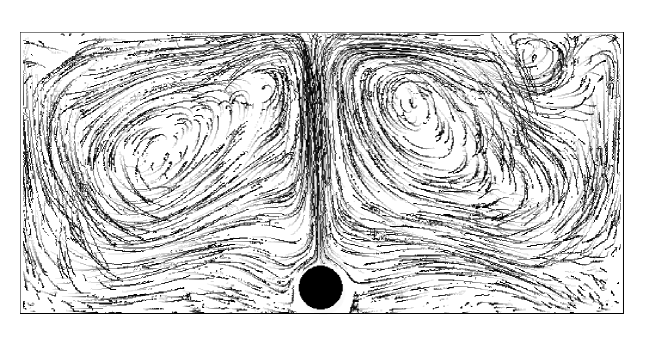
FIG. 18.: An example of trajectories obtained by PTV technique in the convective cell at $Ra=2.39\times 10^{8}$. The vertical thermal plume is clearly observable. The dark circle on the bottom represents the heat source.

The study of Lagrangian dispersion has been done by means of the FSLE [11]. In Figure 19 we plot the result for $Ra=2.39\times 10^{8}$. Again, because there is no scale separation between the Eulerian characteristic scale $l_{0}$ (vortex size) and the basin scale $L$ we cannot expect diffusion behavior. Indeed, the FSLE analysis reveals the chaotic regime $\lambda(\delta)=\lambda$ at small scales and the saturation regime (82) at larger scale.

FIG. 19.: FSLE $\lambda(\delta)$ computed for the convective cell at different initial separations (different symbols). The straight line is the Lyapunov exponent and the dashed curve represents the saturation regime.

The finite scale tool has been successfully applied to many other numerical and experimental situations, from the dispersion in fully developed turbulence, to the analysis of tracer motion in ocean and atmosphere [33, 13, 38], to engineering laboratory experiments. It will be probably became a standard tool in the analysis of Lagrangian dispersion.

REFERENCES

- [1] H. Aref, Ann. Rev. Fluid Mech. 15 345 (1983).
- [2] H. Aref, J. Fluid Mech. 143 1, (1984).
- [3] H. Aref and S. Balachandar, Phys. Fluids, 29, 3515 (1986).
- [4] A.I. Arnold, C. R. Acad. Sci. Paris A, 261, 17 (1965).
- [5] V. Artale, G. Boffetta, A. Celani, M. Cencini and A. Vulpiani, Phys. Fluids A 9 3162 (1997).
- [6] A. Babiano, G. Boffetta, A. Provenzale and A. Vulpiani, Phys. Fluids A 6, 2465 (1994).
- [7] C. Beck and F. Schlögl, Thermodynamics of chaotic systems, Cambridge University Press, Cambridge (1993).
- [8] G. Benettin, A. Giorgilli, L. Galgani and J.M. Strelcyn, Meccanica, 15, 9 and 21 (1980).
- [9] G. Benettin, Physica D 13, 211 (1984).
- [10] L. Biferale, A. Crisanti, M. Vergassola and A. Vulpiani, Phys. Fluids 7, 2725 (1995).
- [11] G. Boffetta, M. Cencini, S. Espa and G. Querzoli, Phys. Fluids 12 3160 (2000).
- [12] G. Boffetta, A. Celani, M. Cencini, G. Lacorata and A. Vulpiani, Chaos 10, 1, 50-60 (2000).
- [13] G. Boffetta, G. Lacorata, G. Redaelli and A. Vulpiani, Physica D, 159, 58-70 (2001).
- [14] G. Boffetta, M. Cencini, M. Falcioni and A. Vulpiani, Physics Reports, 356, Issue: 6, 367-474 (2002).
- [15] C. Boldrighini and V. Franceschini, Commun. Math. Phys., 64, 159 (1979).
- [16] J.P. Bouchaud and A. Georges, Phys. Rep. 195 127 (1990).
- [17] O. Cardoso and P. Tabeling, Europhys. Lett. 7 225 (1988).
- [18] J. Chaiken, C.K. Chu, M. Tabor and Q.M. Tan, Phys. Fluids, 30, 687 (1987).
- [19] M. Cencini, G. Lacorata, A. Vulpiani and E. Zambianchi, J. Phys. Oceanogr. 29, 2578 (1999).
- [20] S. Chandrasekhar, Rev. Mod. Phys. 15, 1 (1943).
- [21] B.V. Chirikov, Phys. Rep. 52, 264 (1979).
- [22] A. Crisanti, M. Falcioni, A. Provenzale and A. Vulpiani, Phys. Lett. A 150, 79 (1990).
- [23] A. Crisanti, M. Falcioni, G. Paladin and A. Vulpiani, Riv. Nuovo Cim. 14 1 (1991).
- [24] A. Einstein, Ann. Phys. (Leipzig) 17, 549 (1905).
- [25] M. Falcioni, G. Paladin and A. Vulpiani, J. Phys. A: Math. Gen., 21, 3451 (1988).
- [26] C.W. Gardiner, Handbook of stochastic methods, 2nd ed. (Springer, Berlin, 1985).
- [27] P. Grassberger and I. Procaccia, Phys. Rev. A, 28, 2591 (1983).
- [28] S. Havlin and D. Ben-Avraham, Adv. Phys. 36 695 (1987).
- [29] M. Hénon, C. R. Acad. Sci. Paris A, 262, 312 (1966).
- [30] Y.H. Ichikawa, T. Kamimura and T. Hatori, Physica D 29 247 (1987).
- [31] M.B. Isichenko, Rev. Mod. Phys. 64 961 (1992).
- [32] A.I. Khinchin, Mathematical foundations of Information theory, Dover (1957).
- [33] G. Lacorata, E. Aurell and A. Vulpiani, Ann. Geophys., 19, 1-9 (2001).
- [34] H. Lamb, Hydrodynamics, New York Dover Publ., New York (1945).
- [35] L.D. Landau and L. Lifshitz, Fluid Mechanics, New York Pergamon Press, New York (1987).
- [36] P. Langevin, Comptes. Rendue 146, 530 (1908).
- [37] J. Lee, Physica D, 24, 54 (1987).
- [38] B. Joseph and B. Legras, To appear in J. Atmos. Sci. (2002).
- [39] C.C. Lin, Proc. Natl. Acad. Sci. U.S. 27, 570 (1941).
- [40] E.N. Lorenz, J. Atmos. Sci. 20, 130 (1963).
- [41] A.J. Majda and P.R. Kramer, Phys. Rep. 314, 237 (1999).
- [42] J.E. Marsden and M. McCracken, The Hopf bifurcation and its applications, MIT Press, Cambridge, Mass. (1975).
- [43] M.R. Maxey and J.J. Riley, Phys. Fluids 26, 883 (1983).
- [44] V.K. Melnikov, Trans. Moscow Math. Soc., 12, 1 (1963).
- [45] H.K. Moffat, Rep. Prog. Phys. 46, 621 (1983).
- [46] A.R. Osborne, A.D. Kirwan, A. Provenzale and L. Bergamasco, Physica D, 23, 75 (1986).
- [47] E. Ott, Chaos in dynamical systems, Cambridge University Press, Cambridge (1993).
- [48] B.I. Shraiman and E.D. Siggia, Nature 405 639 (2000).
- [49] T.H. Solomon and J.P. Gollub, Phys. Fluids 31, 1372 (1988).
- [50] G.I. Taylor, Proc. London Math. Soc. 20, 196 (1921).
- [51] D.J. Tritton, Physical fluid dynamics, Oxford Science Publ., Oxford (1988).
- [52] M. Vergassola, in Analysis and Modelling of Discrete Dynamical Systems, eds. D. Benest & C. Froeschlé, 229 (Gordon & Breach, 1998).
- [53] W. Young, A. Pumir and Y. Pomeau, Phys. Fluids 1 462 (1989).