Soliton Dynamics in Computational Anatomy

Abstract

Computational Anatomy (CA) has introduced the idea of anatomical structures being transformed by geodesic deformations on groups of diffeomorphisms. Among these geometric structures, landmarks and image outlines in CA are shown to be singular solutions of a partial differential equation that is called the geodesic EPDiff equation. A recently discovered momentum map for singular solutions of EPDiff yields their canonical Hamiltonian formulation, which in turn provides a complete parameterization of the landmarks by their canonical positions and momenta. The momentum map provides an isomorphism between landmarks (and outlines) for images and singular soliton solutions of the EPDiff equation. This isomorphism suggests a new dynamical paradigm for CA, as well as new data representation.

I Introduction

Computational Anatomy (CA) must measure and analyze a range of variations in shape, or appearance, of highly deformable structures. Following the pioneering work by Bookstein, Grenander and Bajscy [8, 22, 4], the past several years have seen an explosion in the use of template matching methods in computer vision and medical imaging [53, 51, 54, 3, 14, 25, 36, 55, 56, 24, 33, 40, 39, 38, 30, 37]. These methods have enabled the systematic measurement and comparison of anatomical shapes and structures in biomedical imagery leading to better understanding of neurodevelopmental, neuropsychiatric and neurological disorders in recent years [13, 46, 50, 59, 48, 52, 45, 47, 44, 42, 43, 20, 17, 11, 5, 6]. The mathematical theory of Grenander’s deformable template models, when applied to these problems, involves smooth invertible maps (diffeomorphisms), as presented in this context in [55, 56], [14], [41], [36] and [33]. In particular, the template matching approach involves Riemannian metrics on the diffeomorphism group and employs their projections onto specific landmark shapes, or image spaces.

On the other hand, the diffeomorphism group has also been the focus of special attention in fluid mechanics. For example, Arnold [1] proved that ideal incompressible fluid flows correspond to geodesics on the diffeomorphism group, with respect to the metric provided by the fluid’s kinetic energy. In this paper, we shall draw parallels between these two endeavors, by showing how the Euler-Poincaré theory of ideal fluids can be used to develop new perspectives in CA. In particular, we discover that CA may be informed by the concept of canonical momentum for geodesic flows describing the interaction dynamics for singular solitons in shallow water called peakons [9].

Outline of the paper. Section II describes the template matching variational problems of computational anatomy, and introduces the fundamental EPDiff evolution equation, which describes the evolution of the momentum of an anatomy, (a collection of landmarks, for example). The singular solutions for the EPDiff equation (3) with diffeomorphism group $G$ are explained in section III. They are, in particular, related to the landmark matching problem in computer vision. The consequences of EPDiff for computational anatomy are described in section IV. Conclusions are summarized in section V.

II Variational Formulation of Template Matching Problem

II-A Geometrical large deformation setting.

Grenander [23] pioneered the introduction of group actions in image analysis, through the notion of deformable templates. Roughly speaking, a deformable template is an “object, or exemplar” $I_{0}$ on which a group ${\mathcal{G}}$ acts and thereby generates, through the orbit ${\mathcal{I}}={\mathcal{G}}I_{0}$, a family of new objects. This “template matching” approach has proven to be versatile and useful in different settings (image matching, landmark matching, surface matching and more recently in several extensions of metamorphoses [57]) The approach focuses its modeling effort on properties of the families of shapes generated by the action of the group ${\mathcal{G}}$ on the deformable templates. Right or left invariant geodesic distances on the group ${\mathcal{G}}$ are the natural extension to large deformation of the quadratic cost, or effort function, defined for small linearized perturbations of the identity element.

II-B Case of non-rigid template matching.

The optimal solution to a non-rigid template matching problem is the shortest, or least expensive, path of continuous deformation of one geometric object (template ) into another one (target). For this purpose, we have introduced a time-indexed deformation process, starting at time $t=0$ with the template (denoted $I_{0}$), and reaching the target at time $t=1$. At a given time $t$ during this process, the current object $I_{t}$ is assumed to be the image of the template, $I_{0}$, through the (left) action of a diffeomorphism $\phi_{t}$: $I_{t}=\varphi_{t}\cdot I_{0}$. The attribution of a cost to this process is then based on functionals defined on the group of diffeomorphisms, following Grenander’s principles.

A simple and natural way to assign a cost to a diffeomorphic process indexed by time is based on the following: to measure the variation $\varphi_{t+dt}-\varphi_{t}$, express this difference as a small vector of displacement, $dt\,{\mathbf{u}}_{t}$, composed with $\varphi_{t}$,

$$\varphi_{t+dt}-\varphi_{t}=dt\,{\mathbf{u}}_{t}\circ\varphi_{t}$$

The cost of this small variation is then expressed as a function of ${\mathbf{u}}_{t}$ only, yielding the final expression,

$$\text{Cost}(t\mapsto\varphi_{t})=\int_{0}^{1}\ell({\mathbf{u}}_{t})\,dt$$

with

$$\frac{d\phi_{t}}{dt}={\mathbf{u}}_{t}\circ\varphi_{t}$$ (1)

In the following, the function ${\mathbf{u}}_{t}\mapsto\ell({\mathbf{u}}_{t})$ is defined as a squared functional norm on the infinite dimensional space of velocity vectors. This process is a standard construction in the Riemannian geometry of Lie groups, in which the considered group is equipped with a right invariant Riemannian metric. Here, the vector space of right invariant instantaneous velocities, ${\mathbf{u}}_{t}=(d\phi_{t}/dt)\circ\varphi_{t}^{-1}$, forms the tangent space at the identity of the considered group, and may be regarded as its Lie algebra. This vector space will be denoted $\mathfrak{g}$ in the following (as a formal analogy Lie algebra notation). In this context, the cost of a time-dependent deformation process, thus defined by

$$\text{Cost}(t\mapsto\varphi_{t})=\int_{0}^{1}|{\mathbf{u}}_{t}|_{\mathfrak{g}}^{2}\,dt\,,$$ (2)

is the geodesic action of the process for this Riemannian metric, and most problems in CA can be formulated as finding the deformation path with minimal action, under the constraint that it carries the template to the target. We will illustrate this below with an important example of a such problem, in which the geometric objects are collections of points in space (landmarks). Before doing this, we summarize in more rigorous terms the process described above, providing at the same time the notation to be used in the rest of the paper. However, most of the remaining of the paper can be understood by referring to the summary paragraph at the end of section II-C.

II-C Rigourous construction.

Fix an open, bounded subset $\Omega\subset{\mathbb{R}}^{d}$. Following [55], the construction is based on the design of the “Lie algebra” $\mathfrak{g}$, which is in turn used to generate the group elements. (This is the converse of the usual consideration of finite dimensional Lie groups.) The following construction of $\mathfrak{g}$ will be assumed. Denote by $H$ the set of square integrable vector fields on $\Omega$ with the usual $L^{2}$ metric $(\,\cdot,\cdot\,):\,H\times H\to\mathbb{R}$. Consider a symmetric and coercive operator $L:{\mathbf{u}}\mapsto L{\mathbf{u}}\in H^{*}=H$ whose domain $D(L)$ contains all smooth ($C^{\infty}$) vector fields with compact support in $\Omega$. This operator induces an inner product on $D(L)$ by $\langle{\mathbf{u}},{\mathbf{w}}\rangle_{\mathfrak{g}}=(L{\mathbf{u}},{\mathbf{w}})$. This pre-Hilbert space can be completed to form a Hilbert space ([60]), thereby defining ${\mathfrak{g}}$ which is continuously embedded in $H$ (Freidrich’s extension). Suppose, in addition, that ${\mathfrak{g}}$ can be embedded into $C^{p}(\Omega)$, the set of $p$ times continuously differentiable vector fields on $\Omega$, with $p\geq 1$. (We call this the $p$-admissibility condition.) Then the following can be shown ([55, 14]): If ${\mathbf{u}}_{t}$ is a time-dependent family of elements of ${\mathfrak{g}}$ such that $\int_{0}^{1}\|{\mathbf{u}}_{t}\|^{2}_{\mathfrak{g}}dt<\infty$, that is, ${\mathbf{u}}_{t}\in L^{2}([0,1],{\mathfrak{g}})$, then the flow $\frac{\partial\varphi}{\partial t}={\mathbf{u}}_{t}\circ\varphi_{t}$ with initial conditions $\varphi_{0}(x)=x,\ x\in\Omega$, can be integrated over $[0,1]$, and $\varphi_{1}$ is a diffeomorphism of $\Omega$, which is denoted $\varphi^{\mathbf{u}}_{1}$. The image of $L^{2}([0,1],{\mathfrak{g}})$ by ${\mathbf{u}}\mapsto\varphi^{\mathbf{u}}_{1}$ forms our group of diffeomorphisms, ${\mathcal{G}}$, which is therefore specified by the operator $L$. In this setting, equation (1) has solutions over any finite interval, and the infinum should be taken with respect to $\varphi=\varphi^{\bf u}\circ\varphi_{0}$ for ${\bf u}\in L^{2}([0,1],{\mathfrak{g}})$ such that $\varphi_{1}=\varphi^{\bf u}_{1}\circ\varphi_{0}$. (Because of right-invariance, it can furthermore be assumed that $\phi_{0}=\text{id}$.) Moreover, as proved in [55, 14], the existence of a minimizer (a geodesic path) is guaranteed.

For the inner product $\langle{\mathbf{u}},{\mathbf{w}}\rangle_{\mathfrak{g}}=(L{\mathbf{u}},{\mathbf{w}})$, the operator $L$ is a duality map. In a deformation process $t\mapsto\varphi_{t}$ such that

$$\frac{d\phi_{t}}{dt}={\mathbf{u}}_{t}\circ\varphi_{t}$$

${\mathbf{u}}_{t}$ is called the (Eulerian) velocity, belonging to $\mathfrak{g}$, and $L{\mathbf{u}}_{t}$ is called the momentum, also denoted ${\mathbf{m}}_{t}$. Note that, because $L$ will typically be a differential operator, the momentum $L{\mathbf{u}}$ can (and will) be singular, e.g. a measure, or a generalized function. A simple example of such a phenomenon occurs in the landmark matching problem described in the next subsection.

This framework for CA is reminiscent of the least action principle for continuum motion of fluids with Lagrangian $\ell({\bf u})=\frac{1}{2}\|{\bf u}\|_{\mathfrak{g}}^{2}$. Note that in the template matching framework, $\ell$ has the specific interpretation of an effort functional for small deformations that should be designed according to a given application and not follow any existing physical model. However, this similarity with ideal fluid dynamics sets the stage for “technology transfer” between computational image science and fluid dynamics – e.g., Hamiltonian description, momentum evolution, classification of equilibria, nonlinear stability, PDE analysis, etc. In particular, the least action interpretation of (2), is central in the Arnold theory of hydrodynamics [1] and the derivation of the geodesic evolution equations falls into the Euler-Poincaré (EP) theory, which produces the EP motion equation [27, 41],

$$\Big{(}\frac{\partial}{\partial t}+{\mathbf{u}}\cdot\nabla\Big{)}{\mathbf{m}}+\,\nabla{{\vphantom{\mathbf{u}}}^{t}\mathbf{u}}\cdot{\mathbf{m}}+{\mathbf{m}}({\rm div\,}{\mathbf{u}})=0\,,$$ (3)

and ${\mathbf{u}}=G*{\mathbf{m}}$, where $G*$ denotes convolution with the Green’s kernel $G$ for the operator $L$. This is the EPDiff equation, for “Euler-Poincaré equation on the diffeomorphisms”.

Summary

The important consequences of the previous construction is that, by measuring the amount of fluid deformation which is required to morph an object to another, this measure being given by (2) where $u_{t}$ is the velocity of the fluid deformation at time $t$ and $|{\mathbf{u}}_{t}|_{\mathfrak{g}}^{2}=(Lu_{t},u_{t})$, $L$ being a linear operator, the associated momentum, $m_{t}=Lu_{t}$ satisfies the Euler Poincaré equation (3). This equation is important, because it allows to reconstruct the complete evolution of the momentum (and hence of the fluid motion) from the initial conditions. This property is exploited for the analysis of landmark data in [58].

II-D Landmark matching and measure-based momentum

The landmark matching problem is an interesting illustration of the singularity of the momentum which naturally emerges in the computation of geodesics. Given two collections of points $X_{1},\ldots,X_{K}$ and $Y_{1},\ldots,Y_{K}$ in $\Omega$, the problem consists in finding a time-dependent diffeomorphic process $(t\mapsto\varphi_{t})$ of minimal action (or cost, as given by (2)) such that $\varphi_{0}=\text{id}$ and $\varphi_{1}(X_{i})=Y_{i}$ for $i=1,\ldots,K$. This problem was first addressed in [31], then studied in different forms in [10, 19, 7, 18]. Its computational solution relies on the key observation that the problem can be expressed uniquely in terms of optimizing the landmark trajectories, $\mathbf{Q}_{i}(t)=\varphi_{t}(X_{i})$, for an action, or cost, given by

$$S=\int_{0}^{1}\ell(\mathbf{Q},\mathbf{Q}^{\prime})\,dt=\frac{1}{2}\int_{0}^{1}{{\vphantom{\mathbf{Q}^{\prime}}}^{t}\mathbf{Q}^{\prime}}(t)A(\mathbf{Q}(t))^{-1}\mathbf{Q}^{\prime}(t)\,dt\,,$$ (4)

with notation $\mathbf{Q}^{\prime}(t)=d\mathbf{Q}/dt$. This action, or cost, $S=\int\ell({\bf u})\,dt$ is the time integrated Lagrangian in the least action principle, $\delta S=0$. Its end point conditions are $\mathbf{Q}_{i}(0)=X_{i}$ and $\mathbf{Q}_{i}(1)=Y_{i}$, where $A(\mathbf{Q})$ is an $Kd\times Kd$ matrix ($d$ is the dimension of the underlying space) which may be constructed as follows. Let $G$ be the Green’s kernel associated to the operator $L$, formally defined by

$$\mathbf{v}(x)=\int_{\Omega}G(x,y)(L\mathbf{v})(y)dy\,.$$

Let $I_{d}$ be the $d$-dimensional identity matrix. Then $A(\mathbf{Q})$ is a block matrix $(A_{ij}(\mathbf{Q}),i,j=1,\ldots,K)$ with $A_{ij}(\mathbf{Q})=G(\mathbf{Q}_{i},\mathbf{Q}_{j})I_{d}$.

Denote $\mathbf{P}(t)=A(\mathbf{Q}(t))^{-1}\mathbf{Q}^{\prime}(t)=\partial\ell/\partial\mathbf{Q}^{\prime}$. Then, the optimal diffeomorphism $t\mapsto\varphi_{t}$ is given by equation (1) with

$$\mathbf{u}_{t}(x)=\sum_{i=1}^{K}G(x,\mathbf{Q}_{i}(t))\mathbf{P}_{i}(t)\,.$$

The corresponding momentum $m_{t}$ is given by the point measure

$$\mathbf{m}_{t}(y)=\sum_{i=1}^{K}\mathbf{P}_{i}(t)\delta(y-\mathbf{Q}_{i}(t))\,.$$

A straightforward extension of this model occurs when the landmarks are organized along continuous curves in which the indices $i,j$ are replaced by curve parameters (say defined over $[0,1]$), and

$$\mathbf{m}_{t}(y)=\int_{0}^{1}\mathbf{P}(t,s)\delta(y-\mathbf{Q}(t,s))ds\,.$$

One could also distribute the landmarks along several continuous curves (the outlines of an image, say). This representation of momentum would involve both integrations and sums.

As we will see, this measure-based momentum is also found in other contexts very different from medical imaging. We also mention an important variant of this matching problem. This variant is a particular case of a general framework, in which the diffeomorphic group action is extended to incorporate possible variation in the template itself. The application of this theory of “metamorphoses” [57] to the particular case of landmark matching simply comes with the addition of a new parameter $\sigma^{2}>0$ and the replacement in the above formulas of $A(\mathbf{Q})$ by $A^{\sigma}(\mathbf{Q})=A(\mathbf{Q})+\sigma^{2}I_{Nd}$ ($I_{Nd}$ is the $Nd$ dimensional identity matrix). This corresponds to geodesic interpolating splines introduced in [10]. Note that in this case, EPDiff is not satisfied anymore, but may be modified to include a non-vanishing right-hand term.

III EPDiff and its singular solutions

III-A The EPDiff equation.

The EPDiff equation is important in fluid dynamics, because it encodes the fundamental dynamical properties of energy, circulation and potential vorticity. A first example comes with choosing the differential operator $L$ as $L{\mathbf{u}}=\mathbf{u}$, so that $\mathbf{m}=\mathbf{u}$, and taking incompressible vector fields, so that $\text{div\,}{\mathbf{u}}=0$. In this setting, equation (3) provides the Euler equations for the incompressible flow of an ideal fluid [1, 2].

Another physically relevant form of the EPDiff equation is the evolutionary integral-partial differential equation (3) with [27, 28, 26]

$${\mathbf{m}}\equiv L{\bf u}={\mathbf{u}}-\alpha^{2}\Delta{\mathbf{u}}\,,$$ (5)

so that

$$|\mathbf{u}|_{\mathfrak{g}}^{2}=\|{\mathbf{u}}\|_{H^{1}_{\alpha}}^{2}=\int_{\Omega}(|\mathbf{u}|^{2}+\alpha^{2}|\nabla\mathbf{u}|^{2})dx\,.$$

In this particular case of EPDiff, denoted as EPDiff(H1), one obtains the velocity ${\mathbf{u}}$ from the momentum ${\mathbf{m}}$ by an inversion of the elliptic Helmholtz operator $\big{(}1-\alpha^{2}\Delta)$, with length scale $\alpha$ and Laplacian operator $\Delta$. The EPDiff(H1) equation with momentum definition (5) therefore describes geodesic motion on the diffeomorphism group with respect to $\|{\mathbf{u}}\|_{H_{\alpha}^{1}}^{2}$, the $H_{\alpha}^{1}$ norm of the fluid velocity. This velocity norm is recognized as being (twice) the “kinetic energy,” when equation (3) with momentum definition (5) is interpreted as a model fluid equation, as in shallow water wave theory [27, 28, 29]. Although this operator does not appear in the class of operators used in CA (because it does not satisfy the $p$ admissibility condition), this model exhibits a number of features which are highly relevant also in this case. In particular, singular momentum solutions emerge in the initial value problem for this model which behave as isolated waves, called solitons. In many ways, landmark matching in CA can be seen as generating a soliton dynamics between two sets of landmarks.

III-B Singular momentum solutions of EPDiff.

In the 2D plane, EPDiff, (3), has weak singular momentum solutions that are expressed as [28, 26]

$${\mathbf{m}}({\mathbf{x}},t)=\sum_{a=1}^{N}\int_{s}{\mathbf{P}}_{a}(t,s)\delta\big{(}{\mathbf{x}}-{\mathbf{Q}}_{a}(t,s)\big{)}\,ds\,,$$ (6)

where $s$ is a Lagrangian coordinate defined along a set of $N$ curves in the plane moving with the flow by the equations ${\mathbf{x}}={\mathbf{Q}}_{a}(t,s)$ and supported on the delta functions in the EPDiff solution (6). Thus, the singular momentum solutions of EPDiff are vector valued curves supported on the delta functions in (6) representing evolving “wavefronts” defined by the Lagrange-to-Euler map (6) for their momentum. These solutions have the exact same form as the landmark solutions obtained in the previous section (with the straightforward extension of matching $2N$ curves instead of 2).

Substituting the defining relation ${\mathbf{u}}\equiv G*{\mathbf{m}}$ into the singular momentum solution (6) yields the velocity representation for the wavefronts, as another superposition of integrals,

$${\mathbf{u}}({\mathbf{x}},t)=\sum_{a=1}^{N}\int_{s}{\mathbf{P}}_{a}(t,s)G\big{(}{\mathbf{x}},{\mathbf{Q}}_{a}(t,s)\big{)}\,ds\,.$$ (7)

In the example of EPDiff(H1), the Green’s function $G$ for the second order Helmholtz operator in (5) relates the velocity to the momentum. In this case, the velocity in the singular solution (7) has a discontinuity in its first derivative (its slope) across each curve parameterized by $s$ moving with the flow. Being discontinuities in the gradient of velocity that move along with the flow, these singular solutions for the velocity are classified as contact discontinuities in fluid mechanics. These contact discontinuities do not occur if the Green’s kernel is sufficiently smooth (eg. a Gaussian kernel), as is typically used in CA.

III-C Lagrangian representation of the singular solutions of EPDiff.

Substituting the singular momentum solution formula (6) for $s\in{\mathbb{R}}^{1}$ and its corresponding velocity (7) into EPDiff (3), then integrating against a smooth test function implies the following Lagrangian wavefront equations

$$\frac{\partial}{\partial t}{\mathbf{Q}}_{a}(s,t) = \!\!\sum_{b=1}^{N}\int{\mathbf{P}}_{b}(s^{\prime},t)\,G({\mathbf{Q}}_{a}(s,t),{\mathbf{Q}}_{b}(s^{\prime},t)\,\big{)}ds^{\prime}\,,$$

$$\frac{\partial}{\partial t}{\mathbf{P}}_{a}(s,t) = -\,\!\!\sum_{b=1}^{N}\int{{\vphantom{\mathbf{P}}}^{t}\mathbf{P}}_{a}(s,t)\,{\mathbf{P}}_{b}(s^{\prime},t)$$

$$\hskip 28.45274pt\,\frac{\partial}{\partial{\mathbf{Q}}_{a}(s,t)}G\big{(}{\mathbf{Q}}_{a}(s,t),{\mathbf{Q}}_{b}(s^{\prime},t)\big{)}\,ds^{\prime}\,.$$

Thus, the momentum solution formula (6) yields a closed set of integral partial differential equations given by (III-C) for the vector parameters ${\mathbf{Q}}_{a}(s,t)$ and ${\mathbf{P}}_{a}(s,t)$ with $a=1,2\dots N$. The dynamics (III-C) for these parameters is canonically Hamiltonian and geodesic in phase space.

III-D Relation between contact solutions of EPDiff(H1) and solitons.

As we have discussed, the weak solutions of EPDiff(H1) represent the third of the three known types of fluid singularities: shocks, vortices and contacts. The key feature of these contacts is that they carry momentum; so the wavefront interactions they represent are collisions, in which momentum is exchanged. This is very reminiscent of the soliton paradigm in 1D. And, indeed, in 1D the singular solutions (7) of EPDiff are true solitons that undergo elastic collisions and are solvable by the inverse scattering transform for an isospectral eigenvalue problem [9]. Besides describing wavefronts, this interaction of contacts applies in a variety of fluid situations ranging from solitons [9], to turbulence [12, 15]. The nonlocal elliptic solve ${\mathbf{u}}=G*{\mathbf{m}}$ relating the momentum density ${\mathbf{m}}$ to the velocity ${\mathbf{u}}$ in the EPDiff(H1) equation also appears in the theory of fully nonlinear shallow water waves [9, 21, 28, 29, 49].

The physical concept of momentum exchange is well understood for nonlinear collisions of shallow water waves, especially in 1D. Momentum exchange for EPDiff in 1D is exhaustively studied in [16]. The corresponding momentum exchange processes (wavefront collisions) for EPDiff(H1) in 2D and 3D are studied in [28, 29]. These wavefront collisions show an interesting phenomenon. Namely, wavefront solutions of EPDiff(H1) in 2D and 3D for which a faster wavefront obliquely overtakes a slower one result in the faster wavefront accelerating the slower one and reconnecting with it. Such wavefront reconnections are observed in nature. For example, observations from the Space Shuttle show internal wavefront reconnections occurring in the South China Sea [32]. This wave front reconnection phenomenon is illustrated in Figure 1. The key mathematical feature responsible for wave front reconnection is the nonlocal nonlinearity appearing in EPDiff.

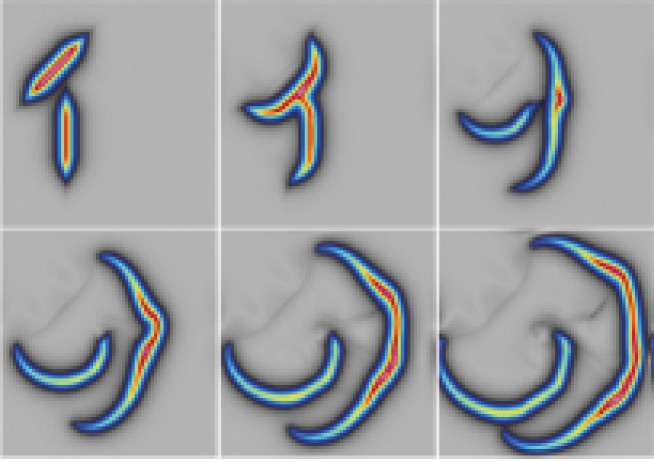
Figure 1: A single collision is shown to produce reconnection as the faster wave front segment initially moving Southwest along the diagonal expands, curves and obliquely overtakes the slower one, which was initially moving rightward (East). This reconnection illustrates one of the collision rules for singular solutions of the two-dimensional EPDiff flow. See [29] for a complete treatment.

III-E $H^{1}_{\alpha}$ norm versus smooth kernels

As noted before, the Green’s kernels for the operators $L$ used in CA are typically smoother than the inverse of the elliptic Helmholtz operator $(1-\alpha^{2}\Delta)$ which corresponds to the $H^{1}_{\alpha}$-model. A consequence of this is that the (variational) matching problems are always well-posed in CA, and their solutions are computationally feasible.

To illustrate the differences introduced by using smooth Green’s kernels, consider the case of a symmetric head-on collision of two particles (or landmarks) in 1D. Under the $H^{1}_{\alpha}$ model, they will meet in finite time, then bounce back after exchanging their momenta. This is impossible with a smooth kernel, since the landmarks are carried by a diffeomorphic motion, and therefore cannot meet if they started from different positions.

III-F Metamorphoses

Interestingly enough, the crossover behavior can be recovered by using metamorphoses, replacing $A$ by $A^{\sigma}$ in (4), because, for this model, particles are slightly disconnected from the diffeomorphic motion, and in this precise situation slightly ahead of it, allowing them to cross without creating a singularity. After crossing, the landmarks carry the diffeomorphism the other way, letting the motion appear like a compression, then a bouncing back after the crossover. To illustrate this, a symmetric frontal shock between two “landmarks” has been simulated in the cases $\sigma=0$ vs. $\sigma>0$ the result is in figure 2.

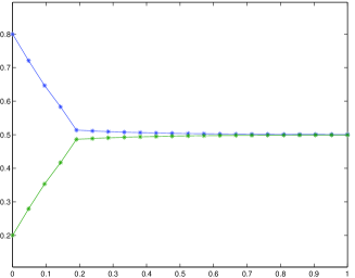
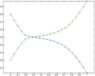
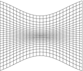
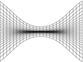
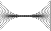
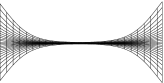
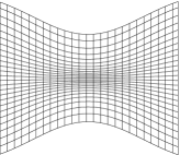
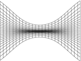
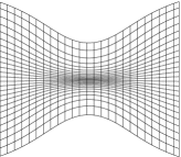
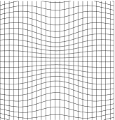
Figure 2: Deformation resulting from a head-on collision of two Gaussian landmarks. First row: $y$ coordinates of the evolving landmarks plotted against time for $\sigma=0$ (left) and $\sigma>0$ (right): contact requires an infinite time when $\sigma=0$, and a crossover is observed in the second case. In the second row, the grid deformation is plotted for the associated 2D deformation, in the exact matching case ($\sigma=0$); The grid gets squeezed while the distance between the landmarks reduces. In this case the deformation is exactly carried by the landmarks. The third row is with $\sigma>0$ (metamorphosis): in this case, the landmarks travel slightly ahead of the deformation, and can cross without creating a singularity. Before the crossover, the grid contracts, then the landmarks diverge and the grid expands.

In 2D, the same behavior can be observed. With a smooth kernel, two expanding circles which have no intersection at time $t=0$ will have no intersection at all times. This is shown in figure 3. When the parameter $\sigma^{2}$ is introduced, the circles intersect in finite time, the value of $\sigma^{2}$ influencing their shapes before and after the collision (figure 4 and 5).

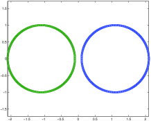
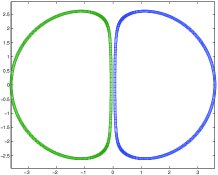
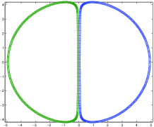
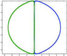
Figure 3: Motion of two expanding circles through EPDiff with a smooth kernel. This corresponds to the case $\sigma=0$ (exact matching). The circles become infinitely close, without crossing.

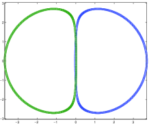
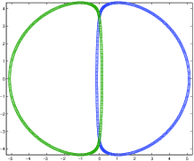
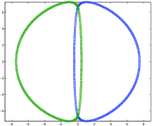
Figure 4: Motion of two expanding circles through metamorphoses with small $\sigma^{2}>0$. The circles intersect in final time, like the landmarks in the head-on collision of figure 2

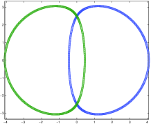
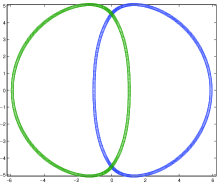
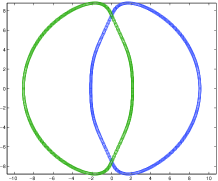
Figure 5: Same as in figure 4, with a larger $\sigma^{2}>0$.

IV Applications of EPDiff in CA.

So far, CA has been related to the issue of comparing two geometric objects, and thus more concerned with the variational “boundary value” problem (2). However, as studied in [34], the initial value problem, associated to the integration of EPDiff, turns out to have very important consequences for applications.

The main consequence of the Euler-Poincaré analysis is that, when matching two geometric structures, the momentum at time $t=0$ contains all the required information for reconstructing the target from the template. This momentum therefore provides a template-centered coordinate system, which essentially encodes all possible deformations which can be applied to it.

There is another important feature which has been observed in the landmark matching problem. Although the momentum is a priori of functional nature, as a result of the application of the operator $L$ to the velocity field ${\mathbf{u}}_{t}$, in the landmark case, we found that it was characterized by a collection of $K$ vectors in space, for a matching problem with $K$ landmarks. Thus, the momentum has exactly the same dimension as the matched structures, and there is no redundancy of the representation. This is generic in the sense that the final dimension of the momentum exactly adapts to the nature of the matching problem. For example, as stated in [34, 35], when matching two smooth scalar images, the momentum has to be normal to the level sets of the image, and therefore is uniquely characterized by its intensity. The momentum can therefore be seen as an algebraic image, which has the same dimension as the original image. This is because template matching brings an additional reduction to the original analysis of finding optimal paths between diffeomorphisms (which leads to the EPDiff equation). This reduction is because the solution must be modded out by the diffeomorphisms that leave the template invariant, which constrains the optimal solution. As a result, the momentum is a (locally) one-to-one representation of the targets, in this template-based coordinate system. It is therefore a non-redundant tool for representing deformations of the template.

Besides being one-to-one, the other advantage of the momentum representation is that it is linear in nature, being dual to the velocity vectors. Thus, linear combinations of either velocity fields, or momenta are meaningful mathematically and physically, provided they are applied to the same template. Thus the average of a collection of momenta, of their principal components, or time derivatives of momenta at a fixed template are all well-defined quantities.

Finally, because they provide an efficient tool for representing deformable data, momenta are perfectly suitable for modeling deformations. Any statistical model on momenta provides, after the integration of EPDiff, a statistical model on deformations, the advantage being that it is much easier to build, sample and estimate statistical models on a linear space. An illustration of this is provided in figure 6, in which the momentum was generated as positive uncorrelated noise on the boundary of a disc, and EPDiff was integrated with this initial conditions. The Green’s function we used for this is a Gaussian kernel, $G(x,y)=\exp(-|x-y|^{2})$. Figure 7 shows the initial momentum of the geodesic path between two 3D sets of landmarks placed on two hippocampi. We also refer to the statistical experiments on PCA in momentum space presented in [58].

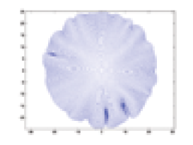
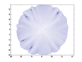
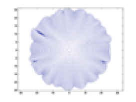
Figure 6: Three deformations of a disc by EPDiff under random initial conditions. These figures visualize the evolution of a disc under the evolution of EPDiff, for initial uncorrelated noise momentum on its boundary. This shows how random deformations in momenta superpose linearly to produce a diffeomorphic change in shape.

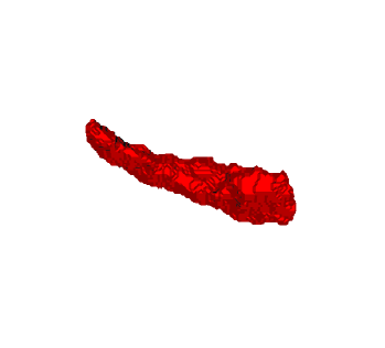
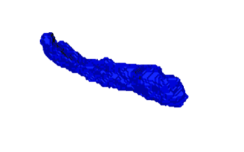
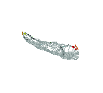
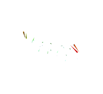
Figure 7: Landmark matching for hippocampi. Two sets of landmarks have been manually defined on the hippocampi in the first row, the first one being considered as the template. The second row shows the initial momentum superimposed with the template (left) and alone (right). Most of the momenta is concentrated at the head and tail of the hippocampus. Data taken from the Biomedical Informatics Research Network (%****␣solitonsInCA.tex␣Line␣925␣****www.nbirn.net)

V Conclusions

We have identified momentum as a key concept in the representation of image data for CA, and discovered important analogies with soliton dynamics. Future work will explore further applications of EPDiff. In particular, it will be interesting to see whether the exchange of momentum in the interactions of multiple outlines will become as useful a concept in computational image analysis as it is in soliton interaction dynamics.

Acknowledgments. DDH is grateful for partial support by US DOE, under contract W-7405-ENG-36 for Los Alamos National Laboratory, and Office of Science ASCAR/AMS/MICS. JTR is grateful for support from NIH (MH60883,MH 62130,P41-RR15241-01A1, MH62626, MH621130-01A1, MH064838, P01-AG03991-16), NSF NPACI and NOHR.

References

- [1] V. I. Arnold. Sur la géométrie différentielle des groupes de lie de dimension infinie et ses applications à l’hydrodynamique des fluides parfaits. Ann. Inst. Fourier (Grenoble), 16(1):319–361, 1966.
- [2] V. I. Arnold and B. A. Khesin. Topological methods in hydrodynamics. Ann. Rev. Fluid Mech., 24:145–166, 1992.
- [3] J. Ashburner, J. G. Csernansky, C. Davatzikos, N. C. Fox, G. B. Frisoni, and P. M. Thompson. Computer-assisted imaging to assess brain structure in healthy and diseased brains. Lancet Neurology, 2:79–88, 2003.
- [4] R. Bajcsy, R. Lieberson, and M. Reivich. A computerized system for the elastic matching of deformed radiographic images to idealized atlas images. J. Comput. Assisted Tomogr., 7:618–625, 1983.
- [5] M. Ballmaier, E. R. Sowell, P. M. Thompson, A. Kumar, K. L. Narr, H. Lavretsky, S. E. Welcome, H. DeLuca, and A. W. Toga. Mapping brain size and cortical gray matter changes in elderly depression. Biol Psychiatry, 55(4):382–9, 2004.
- [6] M. Ballmaier, A. W. Toga, R. E. Blanton, E. R. Sowell, H. Lavretsky, J. Peterson, D. Pham, and A. Kumar. Anterior cingulate, gyrus rectus, and orbitofrontal abnormalities in elderly depressed patients: an mri-based parcellation of the prefrontal cortex. Am J Psychiatry, 161(1):99–108, 2004.
- [7] M. F. Beg. Variational and Computational Methods for Flows of Diffeomorphisms in Image Matching and Growth in Computational Anatomy. PhD thesis, Johns Hopkins University, 2003.
- [8] F. L. Bookstein. Morphometric tools for landmark data; geometry and biology. Cambridge University press, 1991.
- [9] R. Camassa and D. D. Holm. An integrable shallow water equation with peaked solitons. Phys. Rev. Lett., 71:1661–1664, 1993.
- [10] V. Camion and L. Younes. Geodesic interpolating splines. In M. Figueiredo, J. Zerubia, and K. Jain, A, editors, EMMCVPR 2001, volume 2134 of Lecture notes in computer sciences, pages 513–527. Springer, 2001.
- [11] T. D. Cannon, T. G. van Erp, C. E. Bearden, R. Loewy, P. Thompson, A. W. Toga, M. O. Huttunen, M. S. Keshavan, L. J. Seidman, and M. T. Tsuang. Early and late neurodevelopmental influences in the prodrome to schizophrenia: contributions of genes, environment, and their interactions. Schizophr Bull, 29(4):653–69, 2003.
- [12] S. Y. Chen, C. Foias, E. J. Olson, E. S. Titi, and S. Wynne. The Camassa-Holm equations as a closure model for turbulent channel and pipe flows. Phys. Rev. Lett., 81:5338–5341, 1998.
- [13] J. G. Csernansky, M. K. Schindler, N. R. Splinter, L. Wang, M. Gado, L. D. Selemon, D. Rastogi-Cruz, J. A. Posener, P. A. Thompson, and M. I. Miller. Abnormalities of thalamic volume and shape in schizophrenia. Am J Psychiatry, 161(5):896–902., 2004.
- [14] P. Dupuis, U. Grenander, and M. I. Miller. Variational problems on flows of diffeomorphisms for image matching. Quarterly of Applied Math., 56:587–600, 1998.
- [15] C. Foias, D. D. Holm, and E. S. Titi. The Navier-Stokes-alpha model of fluid turbulence. Physica D, 152:505–519, 2001.
- [16] O. Fringer and D. D. Holm. Integrable vs nonintegrable geodesic soliton behavior. Physica D, 150:237–263, 2001. Also available as http://xxx.lanl.gov/abs/solv-int/9903007.
- [17] J. Gee, L. Ding, Z. Xie, M. Lin, C. DeVita, and M. Grossman. Alzheimer’s disease and frontotemporal dementia exhibit distinct atrophy-behavior correlates: a computer-assisted imaging study. Acad Radiol, 10(12):1392–401, 2003.
- [18] J. Glaunès, A. Trouvé, and L. Younes. Diffeomorphic matching of distributions: A new approach for unlabelled point-sets and sub-manifolds matching. In Proceedings of CVPR’04, 2004.
- [19] J. Glaunès, M. Vaillant, and M. I. Miller. Landmark matching via large deformation diffeomorphisms on the sphere. Journal of Mathematical Imaging and Vision, 20:179–200, 2004.
- [20] N. Gogtay, J. N. Giedd, L. Lusk, K. M. Hayashi, D. Greenstein, A. C. Vaituzis, r. Nugent, T. F., D. H. Herman, L. S. Clasen, A. W. Toga, J. L. Rapoport, and P. M. Thompson. Dynamic mapping of human cortical development during childhood through early adulthood. Proc Natl Acad Sci U S A, 101:8174–8179, 2004.
- [21] A. E. Green and P. M. Naghdi. A derivation of equations for wave propagation in water of variable depth. J. Fluid Mech, 78:237–246, 1976.
- [22] U. Grenander. General Pattern Theory. Oxford Science Publications, 1993.
- [23] U. Grenander and M. I. Miller. Representation of knowledge in complex systems (with discussion section). J. Royal Stat. Soc., 56(4):569–603, 1994.
- [24] U. Grenander and M. I. Miller. Computational anatomy: An emerging discipline. Quarterly of Applied Mathematics, LVI(4):617–694, 1998.
- [25] P. Hallinan. A low dimensional model for face recognition under arbitrary lighting conditions. In Proceedings CVPR’94, pages 995–999, 1994.
- [26] D. D. Holm and J. E. Marsden. Momentum maps and measure valued solutions (peakons, filaments, and sheets) of the Euler-Poincaré equations for the diffeomorphism group. In J. E. Marsden and T. S. Ratiu, editors, The Breadth of Symplectic and Poisson Geometry. Birkhäuser, Boston, 2004. to appear.
- [27] D. D. Holm, J. E. Marsden, and T. S. Ratiu. The Euler–Poincaré equations and semidirect products with applications to continuum theories. Adv. in Math., 137:1–81, 1998.
- [28] D. D. Holm and M. F. Staley. Wave structures and nonlinear balances in a family of evolutionary PDEs. SIAM J. Appl. Dyn. Syst., 2(3):323–380, 2003.
- [29] D. D. Holm and M. F. Staley. Interaction dynamics of singular wavefronts in nonlinear evolutionary fluid equations. Technical report, , 2004. In preparation.
- [30] A. K. Jain, Y. Zhong, and M. P. Dubuisson-Jolly. Deformable template models: a review. Signal Processing, 71:109–129, 1998.
- [31] S. C. Joshi and M. I. Miller. Landmark matching via large deformation diffeomorphisms. IEEE transactions in image processing, 9(8):1357–1370, 2000.
- [32] A. K. Liu, Y. S. Chang, M.-K. Hsu, and N. K. Liang. Evolution of nonlinear internal waves in the east and south china seas. J. Geophys. Res., 103:7995–8008, 1998.
- [33] M. I. Miller, A. Trouvé, and L. Younes. On metrics and Euler-Lagrange equations of computational anatomy. Ann. Rev. Biomed. Engng, 4:375–405, 2002.
- [34] M. I. Miller, A. Trouvé, and L. Younes. Geodesic shooting in computational anatomy. Technical report, Center for Imaging Science, Johns Hopkins University, 2003.
- [35] M. I. Miller, A. Trouvé, and L. Younes. The metric spaces, euler equations, and normal geodesic image motions of computational anatomy. In IEEE International Conference on Image Processing, volume 2, pages 635–638, 2003.
- [36] M. I. Miller and L. Younes. Group action, diffeomorphism and matching: a general framework. Int. J. Comp. Vis., 41:61–84, 2001.
- [37] J. Montagnat, H. Delingette, and N. Ayache. A review of deformable surfaces: topology, geometry and deformation. Image and Vision Computing, 19:1023–1040, 2001.
- [38] D. Mumford. Mathematical theories of shape: Do they model perception ? In Proc. SPIE Workshop on Geometric Methods in Computer Vision, volume 1570, pages 2–10. SPIE, Bellingham, WA, 1991.
- [39] D. Mumford. Elastica and computer vision. In Algebraic Geometry and its Applications, pages 507–518. Springer-Verlag, New York, NY, 1994.
- [40] D. Mumford. Pattern theory: a unifying perspective. In Perception as Bayesian Inference, pages 25–62. Cambridge University Press, Cambridge, UK, 1996.
- [41] D. Mumford. Pattern theory and vision. In Questions Mathématiques En Traitement Du Signal et de L’Image, chapter 3, pages 7–13. Institut Henri Poincaré, Paris, 1998.
- [42] K. L. Narr, R. M. Bilder, S. Kim, P. M. Thompson, P. Szeszko, D. Robinson, E. Luders, and A. W. Toga. Abnormal gyral complexity in first-episode schizophrenia. Biol Psychiatry, 55(8):859–67, 2004.
- [43] K. L. Narr, M. F. Green, L. Capetillo-Cunliffe, A. W. Toga, and E. Zaidel. Lateralized lexical decision in schizophrenia: hemispheric specialization and interhemispheric lexicality priming. J Abnorm Psychol, 112(4):623–32, 2003.
- [44] K. L. Narr, T. Sharma, R. P. Woods, P. M. Thompson, E. R. Sowell, D. Rex, S. Kim, D. Asuncion, S. Jang, J. Mazziotta, and A. W. Toga. Increases in regional subarachnoid csf without apparent cortical gray matter deficits in schizophrenia: modulating effects of sex and age. Am J Psychiatry, 160(12):2169–80, 2003.
- [45] K. L. Narr, P. M. Thompson, P. Szeszko, D. Robinson, S. Jang, R. P. Woods, S. Kim, K. M. Hayashi, D. Asunction, A. W. Toga, and R. M. Bilder. Regional specificity of hippocampal volume reductions in first-episode schizophrenia. Neuroimage, 21(4):1563–75, 2004.
- [46] J. A. Posener, L. Wang, J. L. Price, M. H. Gado, M. A. Province, M. I. Miller, C. M. Babb, and J. G. Csernansky. High-dimensional mapping of the hippocampus in depression. Am J Psychiatry, 160(1):83–9., 2003.
- [47] E. R. Sowell, B. S. Peterson, P. M. Thompson, S. E. Welcome, A. L. Henkenius, and A. W. Toga. Mapping cortical change across the human life span. Nat Neurosci, 6(3):309–15, 2003.
- [48] E. R. Sowell, P. M. Thompson, S. E. Welcome, A. L. Henkenius, A. W. Toga, and B. S. Peterson. Cortical abnormalities in children and adolescents with attention-deficit hyperactivity disorder. Lancet, 362(9397):1699–707, 2003.
- [49] C. H. Su and C. S. Gardner. Korteweg-de Vries equation and generalizations. iii. derivation of the Korteweg-de Vries equation and Burgers equation. J. Math. Phys., 10:536–539, 1969.
- [50] R. Tepest, L. Wang, M. I. Miller, P. Falkai, and J. G. Csernansky. Hippocampal deformities in the unaffected siblings of schizophrenia subjects. Biol Psychiatry, 54(11):1234–40., 2003.
- [51] P. M. Thompson, J. N. Giedd, R. P. Woods, D. MacDonald, A. C. Evans, and A. W. Toga. Growth patterns in the developing brain detected by using continuum mechanical tensor maps. Nature, 404(6774):190–3., 2000.
- [52] P. M. Thompson, K. M. Hayashi, G. de Zubicaray, A. L. Janke, S. E. Rose, J. Semple, D. Herman, M. S. Hong, S. S. Dittmer, D. M. Doddrell, and A. W. Toga. Dynamics of gray matter loss in alzheimer’s disease. J Neurosci, 23(3):994–1005, 2003.
- [53] A. W. Toga, editor. Brain warping. Academic Press, 1999.
- [54] A. W. Toga and P. M. Thompson. Temporal dynamics of brain anatomy. Ann. Rev. Biomedical Engng., 5:119–145, 2003.
- [55] A. Trouvé. An infinite dimensional group approach for physics based model. Technical report (electronically available at http://www.cis.jhu.edu), 1995.
- [56] A. Trouvé. Diffeomorphism groups and pattern matching in image analysis. Int. J. of Comp. Vis., 28(3):213–221, 1998.
- [57] A. Trouvé and L. Younes. Metamorphoses through lie group action. Technical report, Center for Imaging Science, Johns Hopkins University, 2004.
- [58] M. Vaillant, M. I. Miller, L. Younes, and A. Trouvé. Statistical analysis of diffeomorphisms via geodesic shooting. NeuroImage, 2004. in press.
- [59] L. Wang, J. S. Swank, I. E. Glick, M. H. Gado, M. I. Miller, J. C. Morris, and J. G. Csernansky. Changes in hippocampal volume and shape across time distinguish dementia of the alzheimer type from healthy aging. Neuroimage, 20(2):667–82., 2003.
- [60] E. Zeidler. Applied Functional Analysis. Applications to mathematical physics. Springer, 1995.