Emergent Effective Collusion in an Economy of Perfectly Rational Competitors

Abstract

We consider a simple model of rational agents competing in a single product market described by simple linear demand curve. Contrary to accepted economic theory, the agents’ production levels synchronise in the absence of conscious collusion, leading to a downward spiraling of market total production until the monopoly price level is realised. This is in stark contrast to the standard predictions of an ideal rational competitive market. Some form of randomness in the form of agent irrationality, or non-synchronous updates is needed to break this emergent “collusion” and return the standard predictions of lower prices in a competitive market.

1. Equilibrium Theory

The standard economic theory of competitive markets argues that the behavior of rational profit-maximizing firms leads to an equilibrium price that equals the marginal cost of production.[Mankiw, 2004] The argument is put in the following way. Firstly, profit for the ith firm in an n-firm industry is defined as:

$$\Pi(q_{i})=P(Q)q_{i}-TC(q_{i}),$$ (1)

where $\Pi(q_{i})$ is the profit of firm $i$ producing quantity $q_{i}$, $P(Q)$ is the market price, which depends only on total production ($Q=\sum_{i}q_{i}$), also known as the demand curve, and $TC(q_{i})$ is the production cost incurred by firm $i$.

Assuming that $P^{\prime}(Q)<0$ (increasing supply reduces prices) and that $TC^{\prime}(q)>0$, it is alleged that profit will be maximised when the derivative of (1) is zero:

$$0=\Pi^{\prime}(q_{\pi_{\max}})=P(Q)+q_{\pi_{\max}}\left.\frac{\partial P}{\partial q_{i}}\right|_{q_{i}=q_{\pi_{\max}}}-TC^{\prime}(q_{\pi_{\max}})$$ (2)

Economists describe $MR(q,Q)\equiv P(Q)+qP^{\prime}(Q)$ as “marginal revenue” and $MC(q)\equiv TC^{\prime}(q)$ as “marginal cost”. In the standard Marshallian theory of markets, all firms are said to maximize profits by equating marginal cost and marginal revenue, independent of the number of firms in the industry—i.e., regardless of whether the industry is a monopoly $(n=1)$, or “competitive”, by which it is meant that $n$ is so large than the $i\mbox{${}^{\mathrm{th}}$}$ firm produces an infinitesimal proportion of total industry output. Firms are also assumed to be managed independently and not react strategically to each other’s behavior, so that $\partial q_{j}/\partial q_{i}=0,\forall i\neq j$ (this assumption is known as atomism). A difference is then alleged to exist between monopolies and competitive industries. Marginal revenue for the monopoly is:

$$P(Q)+QP^{\prime}(Q)<P(Q)$$ (3)

since $P^{\prime}(Q)<0$. Profit-maximizing behavior by a monopoly thus leads to a market price that exceeds the marginal cost of production. On the other hand, each firm in a competitive industry is said to act as a “price-taker” that cannot influence the price in a market, so that $\partial P/\partial q_{i}=P^{\prime}(Q)=0$. Marginal revenue for the $i$^th firm is thus:

$$P(Q)+q_{i}P^{\prime}(Q)=P(Q).$$ (4)

Eq (2) for the competitive firm therefore reduces to

$$P(Q)=TC^{\prime}(q_{\pi_{\mathrm{max}}}),$$ (5)

or in other words the equilibrium price equals marginal cost for the $i$^th firm. Clearly, this can only be an equilibrium if all firms face the same marginal costs, which implies that the aggregate marginal cost of producing industry output $Q$ is equal to the marginal cost faced by each firm producing $q_{i}$. Profit-maximizing by individual firms leads to an aggregate output level at which price equals marginal cost. We denote $Q_{C}$ as the total production level in this case:

$$P(Q_{C})=TC^{\prime}(Q_{C})$$ (6)

In contrast to this standard analysis, Stigler (1957) pointed out that $\partial P/\partial q_{i}$ is not zero, but in fact equal to $P^{\prime}(Q)$, ie $\frac{\partial P}{\partial q_{i}}=\frac{dP}{dQ}\frac{\partial Q}{\partial q_{i}}=\frac{dP}{dQ}$. Therefore equation (5) is incorrect and needs to be revised to:

$$P(Q)-TC^{\prime}(q_{\pi_{\max}})=-q_{\pi_{\max}}P^{\prime}(Q)>0.$$ (7)

Despite its obvious mathematical correctness, most economics textbooks (and economics researchers) do not use this result, but instead continue to argue that $\partial P/\partial q_{i}=0$.. This could be because, as well as pointing out the incompatibility of the assumption of “price-taking” behavior ($\partial P/\partial q_{i}=0$) in the context of atomism ($\partial q_{j}/\partial q_{i}=0,\forall i\neq j$), Stigler also proposed a reformulation of marginal revenue in the symmetric case $q_{i}=q,\,\forall i$, that appeared to describe eq (5) as the limit of profit-maximizing behavior as $n\rightarrow\infty$:

$$P(Q)+q_{i}P^{\prime}(Q)=P\left(1+\frac{1}{nE}\right)$$ (8)

($E=\frac{P}{Q}\frac{dQ}{dP}$ is called the market elasticity of demand). Marginal revenue for the individual competitive firm therefore converges to market price as $n\rightarrow\infty$. On the presumption that profit maximizing behavior involves equating marginal revenue and marginal cost, the $n$-firm economy approaches the Cournot equilibrium (5) as $n\rightarrow\infty$ (however, this also implies that $q_{i}\rightarrow 0$ in this same limit).

However, using Stigler’s relation, Keen (2003) shows that equating marginal cost and marginal revenue does not maximize profits in a multi-firm industry. Keen’s method was proof by contradiction: assuming that all firms did equate marginal cost and marginal revenue, Keen showed that this resulted in an aggregate output that exceeded the profit-maximizing level. Therefore part of industry output had to be produced at a loss, which in turn meant that some individual firms had to be producing beyond their profit-maximizing output. Summarizing this analysis, if all firms equate marginal revenue and marginal cost, then

$$\sum_{i}\left(P(Q)+q_{i}P^{\prime}(Q)-MC(q_{i})\right)=0$$ (9)

$$\Rightarrow nP(Q)+QP^{\prime}(Q)-nMC(Q)=0$$

$$\Rightarrow MR(Q,Q)-MC(Q)=-(n-1)\left(P(Q)-MC(Q)\right),$$

which is negative by virtue of Stigler’s relation (7). This aggregate output level exceeds the profit maximizing level, since aggregate marginal cost exceeds aggregate marginal revenue. This relation quantifies the aggregation fallacy in the proposition that firms maximize their profit by setting the partial derivative of their profit with respect to their own output to zero when in a multi-firm industry the equilibrium profit level is found by setting the total derivative of each firm’s profit to zero:

$$\frac{d\Pi(q_{i})}{dQ}=\sum_{j}\frac{\partial\Pi(q_{i})}{\partial q_{j}}\frac{\partial q_{j}}{\partial Q}=P(Q)+nq_{i}P^{\prime}(Q)-MC(q_{i})=0$$ (10)

We can express this equation as

$$q_{i}P^{\prime}(Q)=-\frac{1}{n}\left(P(Q)-MC(q_{i})\right).$$ (11)

and

$$P(Q)+q_{i}P^{\prime}(Q)-MC(q_{i})=-(n-1)q_{i}P^{\prime}(Q)$$ (12)

Substituting (11) into (12), we arrive at the following condition for the profit-maximizing equilibrium (which we call the Keen equilibrium rather than the “monopoly” equilibrium as economists normally describe it) [Keen, 2004b, Keen, 2004a]. Denoting the total market production in this case by $Q_{K}$, each firm’s output satisfies:

$$P(Q_{K})+q_{i}P^{\prime}(Q_{K})-MC(q_{i})=\frac{n-1}{n}\left(P(Q_{K})-MC(q_{i})\right)$$ (13)

This formula corresponds to the accepted formula for a monopoly, but in the $n$-firm case, firms produce at levels where their own-output marginal revenue exceeds their marginal cost. It is easily shown that this formula maximizes profit for any total revenue and total cost functions that obey the standard conditions $P^{\prime}(Q)<0$ and $TC^{\prime}(q)>0$.

In what follows, we use multi-agent modelling to (a) dispute the “given other firms’ outputs fixed” definition of rationality, (b) show that the Cournot equilibrium is locally unstable while the Keen equilibrium is locally stable, (c) establish that operationally rational profit-maximizing behavior leads to the Keen equilibrium, and (d) quantify the degree of operationally irrational behavior needed for the output to converge to the Cournot equilibrium. The behavior of the agents and the overall system illustrates an interesting phenomenon in multi-agent dynamics: the emergence of apparently coordinated behavior even though agents are not colluding or even communicating with each other.

2. Dynamics

With the assumption that $\partial P/\partial q_{i}=0$, eq (2) asserts that each firm works in isolation. Each firm considers what is the optimal level of production on the assumption that the production levels of all other firms remain fixed. Yet this is a contradictory situation, as every firm is attempting to adjust its production levels to maximise its profit at the same time. Rational firms, who are themselves adjusting their own outputs in a search for the level that maximises profits, are in effect assumed to irrationally believe that other firms are not doing the same thing. Therefore in each time period, the total market production $Q$ cannot be predicted.

While it is possible that aggregate historical data exists (production levels and prices) that might allow a demand curve to be deduced, this is of little help in the competitive setting. Rational agents performing optimisation according to eq (2) cannot exist since each behaves as if it has no impact on market price, and therefore no market price can therefore be determined: the price would be what it always was — “Que sera sera” — without any tendency to move. The actual equilibrium production values (if an equilibrium exists) must arise in a dynamical setting where agents make decisions based on limited knowledge and where, however small, their actions have an impact on their own situation and therefore the aggregate market outcome. Obviously there is a need to examine how real firms make decisions, however it is theoretically instructive to consider the ideal case of simple firms making rational decisions based on information available.

In this paper, we assume the only information a firm has is its own cost function, the decision it made on the previous time step (increase or decrease production), and what impact this decision had on its profit levels. The obvious operationally rational use of this information is to continue changing levels of production in the same direction if profits are rising, and to reverse the direction of change if profits fall. To make the opposite decision, to “buck the trend” in other words, is to discard any trend information that might be contained within the profit time series.

It is difficult to follow analytically the outcome of more than two interacting firms. The equilibrium theory described in §1. is assumed to be valid in the limit of an infinite number of firms. Therefore, we resort to numerical simulations to explore what happens as the number of firms is increased. In the following numerical simulations, we use affine demand and cost rules:

$$P(Q) =a-bQ=100-10^{-2}Q$$ (14)

$$TC(q) =cq=50q$$ (15)

For this model, the Cournot and Keen Equilibria can be computed from eq (6) and (13):

$$Q_{C}=(a-c)/b=5000 ;P(Q_{C})=50$$ (16)

$$Q_{K}=(a-c)/2b=2500 ;P(Q_{K})=75$$ (17)

In this model, $Q_{K}$ corresponds to the monopoly production levels. The code used for this simulation is available from the author’s website.

Figure 1 shows the convergence to monopoly prices for a number of different economy sizes. The simulations were started at the Cournot level in each case, and rapidly converged to the monopoly levels.

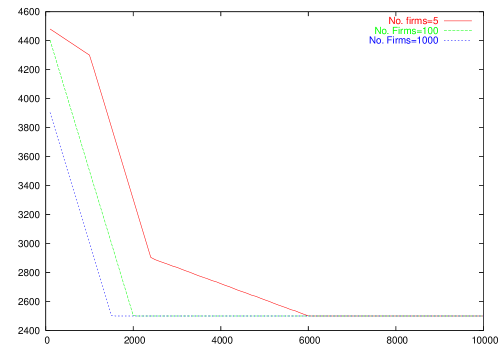
Time

Market Production

Figure 1: Total market production starting at $Q=4500$ for different sizes of economy. The different slopes on the $n=5$ curve correspond initially to only 3 firms synchronised, then 5 firms, then finally several firms overshoot their share of the final production and begin to increase production, slowing the final approach to equilibrium. The precise shape of the curve depends on the initial distribution of increments, which is assigned randomly.

It is instructive to consider the two firm case to understand what is going on [Simon et al., 1973]. Consider first the case where both firms have been initialised to a production of $q>Q_{K}/2=(a-c)/4b$ with a negative increment $\delta$. They will then both decrease production, leading to increased profits for both firms.

$$\Pi(q-\delta) =(a-c)(q-\delta)-2b(q-\delta)^{2}$$

$$=\Pi(q)-(a-c-4bq)\delta-2b\delta^{2}$$ (18)

$$>\Pi(q)$$ (19)

Since they are acting rationally, they will continue this action until global profit maximisation is reached — the monopoly situation.

If, however, both firms are initialised with a positive increment, both firms will immediately increase production, leading to falling profit levels. Since they are both acting perfectly rationally, they will then both switch to negative increments, leading to increased profits which will converge on the monopoly outcome as before.

Finally, consider the case of the firms being initialised with opposing increments, with $q<Q_{C}/2=(a-c)/2b$:

$$\Pi(q-\delta) =(a-c)(q-\delta)-2bq(q-\delta)$$

$$=\Pi(q)-(a-c-2bq)\delta$$ (20)

$$<\Pi(q)$$

$$\Pi(q+\delta) =(a-c)(q+\delta)-2bq(q+\delta)$$

$$=\Pi(q)+(a-c-2bq)\delta$$ (21)

$$>\Pi(q).$$ (22)

Then the firm with the negative increment will switch to a positive increment and we are back in the previous situation of both firms having the same increment. Exactly the same situation pertains with $q>Q_{C}/2$, except that the firm with positive increment switches to a negative increment. The end result is monopoly levels.

Only in the case $q=Q_{C}/2=(a-c)/2b$ do production levels remain constant at the Cournot level. It turns out that this “metastable” state is sensitive to numerical rounding in the model. The probability of this happening in an initialisation decreases as $2^{-n/2}$ as the number of firms $n$ increases, and cannot happen for odd $n$.

The interesting thing to note is that it is the agent’s rationality which causes the two agents to lock into a spiral of lower production levels and increased prices. If at any stage during this process, one agent were to ramp up production, they could increase their own production at the expense of the other party. The other party would quickly follow suit, and the two agents would then reenter the downward spiral again. As a result, the interactive topography of the profit landscape makes the Keen equilibrium locally stable for the two agents, while the Cournot equilibrium is locally unstable. This can be seen by considering the impact of changes in output on profit levels for the two firms in the vicinity of these equilibria. Tables 1 and 2 show the impact of changing output by one and two units by each firm in the vicinity of the Keen and Cournot equilibria respectively. The only changes which are viable are ones in which both profit change entries are positive, since where a negative change occurs the firm experiencing this change will reverse its direction of output change. As can be seen from Table 1, there is no change in output combination which is viable: a change in any direction by either firm results in at least one change in profit figure that is negative. Therefore the firm experiencing this change will alter its direction of output change, thus returning the collective output level to the Keen equilibrium figure.

		Firm B
		$-2$	$-1$	0	1	2
	$-2$
Firm A	$-1$
	$0$
	$1$
	$2$

Table 1: Table showing the change in profits for two companies around the Keen equilibrium, for $\Delta q_{i}=\pm 1,\pm 2$.

On the other hand, there is a viable direction of output change from the Cournot equilibrium shown in Table 2: if both firms reduce their output, then both will experience an increase in profits. Hence a reduction in output by both firms is a viable strategy for each firm acting independently, and the firms will therefore move away from the Cournot equilibrium. The Cournot equilibrium is therefore locally unstable, while the Keen equilibrium is locally stable.

		Firm B
		$-2$	$-1$	0	1	2
	$-2$
Firm A	$-1$
	$0$
	$1$
	$2$

Table 2: Table showing the change in profits for two companies around the Cournot equilibrium, for $\Delta q_{i}=\pm 1,\pm 2$.

The $n$-firm case is similar. It only takes more than 50% of the agents to be simultaneously decreasing production to reduce the total market production, which will lead to increased profits for all. Even though none of the agents are communicating with each other, the effect is as if they were colluding with each other to keep market prices high.

3. Variant Dynamics

3.1 Irrational Dynamics

Figure 2 plots the effect of irrationality versus number of firms. Irrationality governs the probability that an agent makes the opposite decision to the rational one. It can be seen that quite high levels of irrationality are required to break the trend towards monopoly valued economies. There is a fairly sharp transition between the system being pulled to the Keen equilibrium in the rational case, and the Cournot equilibrium when irrationality lies between 0.3 and 0.5 for many firms. If the firms are more than 50% irrational then neither equilibrium is an attractor, as firms are no longer profit seeking.

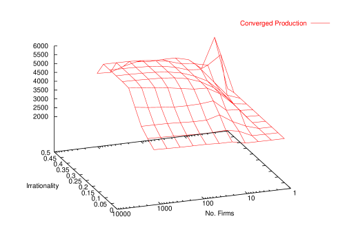
Figure 2: Plot of the converged production levels as a function of irrationality and number of firms. Converged production level is computed as the average production value $Q$ between $t=40000$ and $t=50000$.

3.2 Update rules

Until now we’ve been considering the effect of all firms updating production levels every timestep. The opposite extreme of only one firm updating its production level leads to the ideal situation considered for the Cournot equilibrium. Interpolating between the two cases, we can consider dynamics where only a fraction of firms update there production rules in any timestep, selected at random from the list of all firms. Figure 3 shows the converged production values as a function of the proportion of firms updating each timestep, and number of firms.

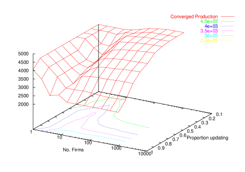
Figure 3: Plot of the converged production levels as a function of the number of firms, and the proportion of those firms updating their production levels each timestep. Converged production level is computed as the average production value $Q$ between $t=40000$ and $t=50000$.

This outcome occurs because when each firm alters its output while other firms hold theirs constant, the change in revenue to which the firm reacts is its own-output marginal revenue, as defined above. This will indicate to the firm that it can increase its profit by increasing its output from the Keen level, in a process which terminates at the Cournot equilibrium.

However, this behavior is both unrealistic (other firms do not hold their output while one firm varies its in the real world), and involves a peculiar form of irrationality—since though the change in output is done with the intention of increasing profit, over each iteration it results in the firm’s profit level falling, once all other firms have done likewise. Thus what appears rational within each iteration becomes irrational from one iteration to the next. A less myopic behavioral rule—which included consideration of the profit outcome from one iteration to the next—would probably reverse this behavior. In this work, only the result from the last and last but one market outcome is used in determining the agents’ behaviour. It is, of course, clearly possible to make use of more market historical data, say the results of the last $\ell>2$ market periods. It is not clear, in this case, what the response of a rational agent should be. One possibility is a lookup decision table indexed by the relative movements of the market over the last $\ell$ periods, analogous to the minority game [Challet and Zhang, 1997].

The stability of this myopic sequential update rule is also dependent on the percentage of firms that change output at each timestep. For large economies ($>32$ firms), the system converges to the Cournot equilibrium (5000) when only 10% of the firms are updating their production levels per timestep, and to the Keen equilibrium when all firms are updating their production levels. The final production levels shows a smooth decline as the percentage of firms updating increases.

The somewhat strange behaviour at small economy sizes can be explained by the fact that individual firms have proportionately larger effects on total production values, so only a few firms need to synchronise to pull production levels down to monopoly values. In the single firm case, no firms are updating at all, so final values are simply the initial values of 4500.

4. Conclusion

The simulation results demonstrate that markets can be locked in a spiral of restricted production converging on monopoly pricing levels as though the firms were colluding, even though no interaction between firms takes place. Perfect profit-seeking rationality and the dynamics of the economy tends to lock firms into synchronous behaviour, leading to a global monopoly behaviour. Only by inserting some randomness in the system by way of irrationality, or by decoupling the firm’s production periods, does the economy “melt” into the behaviour predicted by competition theory. Clearly such factors may operate in real markets, and this work does not suggest that real competitive markets will produce monopolistic outcomes, but it does suggest that the ideal perfectly rational competitive market does not produce the expected competitive outcomes.

5. Acknowledgments

The authors would like to thank the Australian Centre for Advanced Computing and Communications for access to a large Linux cluster that enabled the simulations to be completed in a timely manner.

References

- [Challet and Zhang, 1997] Challet, D. and Zhang, Y.-C. (1997). Emergence of cooperation and organization in an evolutionary game. Physica A, 246:407.
- [Keen, 2003] Keen, S. (2003). Standing on the toes of pigmies: Why econophysics must be careful of the economic foundations on which it builds. Physica A, 324:108–116.
- [Keen, 2004a] Keen, S. (2004a). Deregulator: Judgment day for microeconomics. Utilities Policy, 12:109.
- [Keen, 2004b] Keen, S. (2004b). Why economics must abandon its theory of the firm. In Salzano, M. and Kirman, A., editors, Economics: Complex Windows. Springer, New York.
- [Mankiw, 2004] Mankiw, G. N. (2004). Principles of Microeconomics. Thomson/South-Western, Mason, Ohio.
- [Mas-Collell et al., 1995] Mas-Collell, A., Whinston, M., and Green, J. (1995). Microeconomic Theory. Oxford UP, New York.
- [Simon et al., 1973] Simon, J. L., Puig, C. M., and Aschoff, J. (1973). A duopoly simulation and richer theory: an end to Cournot. Review of Economic Studies, 40:353–366.
- [Stigler, 1957] Stigler, G. J. (1957). Perfect competition, historically contemplated. The Journal of Political Economy, 65:1–17.
- [Varian, 1999] Varian, H. (1999). Intermediate Microeconomics: A Modern Approach. WW Norton, New York.