Optical-parametric-oscillator solitons driven by the third harmonic

Abstract

We introduce a model of a lossy second-harmonic-generating ($\chi^{(2)}$) cavity externally pumped at the third harmonic, which gives rise to driving terms of a new type, corresponding to a cross-parametric gain. The equation for the fundamental-frequency (FF) wave may also contain a quadratic self-driving term, which is generated by the cubic nonlinearity of the medium. Unlike previously studied phase-matched models of $\chi^{(2)}$ cavities driven at the second harmonic (SH) or at FF, the present one admits an exact analytical solution for the soliton, at a special value of the gain parameter. Two families of solitons are found in a numerical form, and their stability area is identified through numerical computation of the perturbation eigenvalues (stability of the zero solution, which is a necessary condition for the soliton’s stability, is investigated in an analytical form). One family is a continuation of the special analytical solution. At given values of parameters, one soliton is stable and the other one is not; they swap their stability at a critical value of the mismatch parameter. The stability of the solitons is also verified in direct simulations, which demonstrate that the unstable pulse rearranges itself into the stable one, or into a delocalized state, or decays to zero. A soliton which was given an initial boost $C$ starts to move but quickly comes to a halt, if the boost is smaller than a critical value $C_{\mathrm{cr}}$. If $C>C_{\mathrm{cr}}$, the boost destroys the soliton (sometimes, through splitting into two secondary pulses). Interactions between initially separated solitons are investigated too. It is concluded that stable solitons always merge into a single one. In the system with weak loss, it appears in a vibrating form, slowly relaxing to the static shape. With stronger loss, the final soliton emerges in the stationary form.

PACS numbers: 42.65.Yj; 42.65.Tg; 05.45.Yv

1 Introduction

In the vast family of optical solitons, an important niche is occupied by solitary waves in cavities, supported by the quadratic ($\chi^{(2)}$) nonlinearity of the degenerate optical-parametric-oscillator (OPO) type [1, 2]. The intrinsic loss in the cavity should be compensated by an external pump field $E$, which in most cases is supplied at the second harmonic (SH) [3]. Such an arrangement is frequently referred to as downconversion, and is described by the model in which either the evolution equation for the SH field $v$ explicitly contains a constant driving term $\sim E$, [4, 5], or, equivalently, the equation for the fundamental-frequency (FF) wave $u$ includes a parametric-gain term $\sim Eu^{\ast}$, where the asterisk stands for the complex conjugation [6, 7, 8]. Alternatively, the cavity may be externally pumped at the FF, which is referred to as upconversion, the respective model including a constant driving term in the FF equation [9]. For both cases, families of one-dimensional solitons and their stability have been investigated in detail, see Refs. [4]-[10] and references therein. The stability of cavity solitons was tested in a direct experiment using the photorefractive nonlinearity [11].

It should be mentioned that, as the cavity models are dissipative ones, the solitary pulses found in these models are not solitons in the rigorous sense. Nevertheless, this term is broadly applied to them, therefore we use it in this paper too.

The analysis of solitons in OPO models was extended in various directions, including the study of moving solitons [12], interactions between them [13], nondegenerate second-harmonic-generation (SHG) which involves two FF waves with orthogonal polarizations [14], general three-wave interactions [15], the use of the quasi-phase-matching technique [16], two-dimensional solitons (see, e.g., Ref. [17]), etc. Besides their significance as the subject of fundamental research, OPO cavity solitons also have a potential for the design of rewritable multi-pixel optical-memory patterns [18].

In this work, we aim to propose and analyze another possibility to drive dissipative cavities with the SHG nonlinearity, namely, through a phase-matched third-harmonic (TH) pump wave, $w$. Obviously, the corresponding driving terms in the equations for the FF and SH fields $u$ and $v$, which are generated by the parametric interaction of these fields with the TH pump, are proportional, respectively, to $wv^{\ast}$ and $wu^{\ast}$. Thus, this model includes a new feature, the cross-parametric gain, in the system of coupled FF and SH waves, and a problem of straightforward interest is to study solitons that can be supported by this type of the gain in the lossy SHG setting, especially as concerns stability of the solitons. Besides that, we will also take into regard a possibility of an additional quadratically nonlinear parametric self-driving term in the equation for the FF field $u$, in the form of $w\left(u^{\ast}\right)^{2}$, which may be induced by the same TH pump through the $\chi^{(3)}$ (cubic) nonlinearity. In this work, we consider only bright solitons; dark solitons, and patterns in the form of domain walls (see, e.g., Ref. [19]) may also be possible in the model including the TH drive.

As concerns the mutual phase matching between the FF, SH, and TH fields, which is implied in the model, it was demonstrated, in another context, that matching of this type may take place in the so-called multi-step $\chi^{(2)}$ systems [20]. However, the subject of Ref. [20] was the corresponding three-wave solitons, rather than pumping of the FF and SH fields through the TH wave.

The paper is organized as follows. In Section II, we give the formulation of the model, and find particular exact solutions for the solitons in an analytical form. In the same section, we also investigate stability conditions for the zero solution, which is a necessary prerequisite for the stability of solitons. In Section III, we find two families of general soliton solutions in a numerical form. One family is a direct continuation of the exact solution, while the other one is different. As well as the analytically found soliton, they always have a single-humped shape, but, unlike the constant-phase exact solutions, they feature intrinsic chirp. Stability regions for the solitons are identified, in the system’s parameter space, through computation of the corresponding eigenvalues for small perturbations. One of the solitons is stable, and the other one is not; they swap the stability via a bifurcation at a critical value of the mismatch parameter. The shape of the stability regions is quite nontrivial; in the model with weak losses, the stable solitons may have complex eigenvalues, corresponding to weakly damped intrinsic oscillatory modes. The stability is also verified in direct simulations, with a conclusion that the unstable soliton rearranges into the stable one, or into a delocalized spatially periodic state, or, sometimes, it decay to zero. Also in Section III, we show that attempts to produce moving solitons fail: if the soliton is initially boosted by lending it a speed $C$, it quickly stops, provided that $C$ is smaller than a critical value $C_{\mathrm{cr}}$; the boost with $C>$ $C_{\mathrm{cr}}$ destroys the soliton. Section IV deals with interactions between two stable solitons, initially placed at some distance. They merge into a single soliton, which emerges with slowly fading intrinsic vibrations in the weakly dissipative model, or immediately in the stationary form if the loss parameter is larger. Section V discusses possible extensions of the work and concludes the paper.

2 The model and exact results

Equations which describe the degenerate $\chi^{(2)}$ interaction between the FF and SH fields $u(x,t)$ and $v(x,t)$ in a one-dimensional lossy cavity in the presence of an additional pump TH wave $w_{0}$, whose depletion is negligible, are straightforward to derive:

$$i\omega_{0}u_{t}+\frac{1}{2}u_{xx}+\chi^{(2)}u^{\ast}v = \left(q_{1}-i\alpha_{1}\right)u+iw_{0}v^{\ast}+i\chi^{(3)}w_{0}\left(u^{\ast}\right)^{2},$$ (1)

$$2i\omega_{0}v_{t}+\frac{1}{2}v_{xx}+\frac{1}{2}\chi^{(2)}u^{2} = 2\left(q_{2}-i\alpha_{2}\right)v+iw_{0}u^{\ast}.$$ (2)

Here, $\omega_{0}$ is the fundamental carrier frequency, the coefficient amenable for the three-wave coupling between the FF, SH and TH fields is absorbed into $w_{0}$, $q_{1}$ and $q_{2}$ are real detuning coefficients at the FF and SH, and $\alpha_{1}$ and $\alpha_{2}$ are the loss coefficients for the same fields. In this paper, we focus on the most natural case, $\alpha_{1}=\alpha_{2}$, but the analysis has demonstrated that the results do nor differ in any noticeable aspect for $\alpha_{1}\neq\alpha_{2}$. The last term in Eq. (1) takes into regard the above-mentioned possibility of the nonlinear parametric self-driving of the FF field, which can directly couple to the TH pump wave in the presence of the cubic nonlinearity. The factors of $i$ in front of the cross-parametric-driving terms in Eqs. 1) and (2), while $w_{0}$ is assumed real, can always be fixed, defining phase shifts between the corresponding waves.

After obvious normalizations (in particular, the SH field is rescaled with $u\rightarrow\sqrt{2}u$, so as to keep the coefficients in front of the cross-driving terms equal in the two equations), Eqs. (1) and (2) can be cast in the following form:

$$iu_{t}+\frac{1}{2}u_{xx}+u^{\ast}v = \left(1-i\alpha_{1}\right)u+i\alpha_{0}v^{\ast}+i\beta\left(u^{\ast}\right)^{2},$$ (3)

$$iv_{t}+\frac{1}{4}v_{xx}+\frac{1}{2}u^{2} = \left(2q-i\alpha_{1}\right)v+i\alpha_{0}u^{\ast},$$ (4)

where $\alpha_{0}$ and $\beta$ are the effective pumping coefficients, both proportional to $w_{0}$, the mismatch coefficient in Eq. (3) is normalized to be $1$ (a different variant of the model is obtained by fixing the latter coefficient to be $-1$, but the existence of bright solitons is not expected in that case). The notation for the fields $u$ and $v$ and the coefficient $\alpha_{1}$ was not altered, although they were rescaled (recall we assume $\alpha_{2}=\alpha_{1}$). By means of a phase shift of $u$ and $v$, $\alpha_{0}$ may always be made real, which we assume below, while $\beta$ is, generally speaking, a complex coefficient.

Obviously, Eqs. (3) and (4) cannot give rise to stable localized solutions unless the zero solution, $u=v=0$, is stable. Linearizing the equations, an elementary calculation yields the following stability condition for the zero solution:

$$\alpha_{0}^{2} \leq \alpha_{1}^{2}+\left(1+2q\right)^{2}/4,~{}\mathrm{if}~{}~{}1+2q>0;$$

$$\alpha_{0}^{2} \leq \alpha_{1}^{2},~{}\mathrm{if}~{}~{}1+2q<0.$$ (5)

The consideration of the linearized version of Eqs. (3) and (4) makes it also possible to predict the asymptotic form of the exponentially decaying tails of the soliton solution at $|x|~{}\rightarrow\infty$,

$$\left(u,v^{\ast}\right)\sim\exp\left(-\lambda|x|\right),$$ (6)

where a (generally) complex constant $\lambda$ (it is defined so that its real part is positive) is to be found from the equation

$$\left(\frac{1}{2}\lambda^{2}-1+i\alpha_{1}\right)\left(\frac{1}{4}\lambda^{2}-2q-i\alpha_{1}\right)=\alpha_{0}^{2}~{}.$$ (7)

The complex structure of $\lambda$ implies that the soliton must have a nontrivial intrinsic phase structure, which will be studied in detail below.

Particular exact soliton solutions to Eqs. (3) and (4) can be sought for as

$$u_{0}(x)=A\,e^{i\phi}\mathrm{sech}^{2}\left(\kappa x\right),\,\,v_{0}(x)=B~{}e^{2i\phi}\mathrm{sech}^{2}\left(\kappa x\right),$$ (8)

where $\kappa$, $\phi$ and $A$, $B$ are real constants. This ansatz may produce solutions in the case of $\beta=0$ [no self-driving quadratic term in Eq. (3)]. Then, the soliton’s parameters are obtained by direct substitution of the expressions (8) into Eqs. (3) and (4):

$$\kappa^{2}=1-2q,$$ (9)

$$A=B=3\kappa^{2},$$ (10)

$$\cos\left(3\phi\right)=\alpha_{1}/\alpha_{0}\,,~{}\sin\left(3\phi\right)=\left(1-4q\right)/\alpha_{0}\,~{}.$$ (11)

Due to the identity $\sin^{2}\left(3\phi\right)+\cos^{2}\left(3\phi\right)\equiv 1$, Eqs. (11) give rise to an additional constraint on the parameters of the model which is necessary for the existence of the exact solution in the above form,

$$\alpha_{0}=\left(\alpha_{0}\right)_{\mathrm{exact}}\equiv\sqrt{\alpha_{1}^{2}+\left(1-4q\right)^{2}}.$$ (12)

Equation (12) determines the value of the cross-parametric-gain which is necessary to support the exact soliton solution. Thus, the two conditions, $\beta=0$ and (12), must be imposed on the parameters of Eqs. (3) and (4) to provide for the existence of the analytical solution for the soliton in the simple form (8) (in fact, the condition $\alpha_{1}=\alpha_{2}$, which was adopted above, is also necessary for the existence of the exact soliton in the present form).

It is relevant to notice that, comparing Eq. (8) with the asymptotic waveform (6), one can identify, for the present solution, $\lambda=2\kappa$. Then, taking into regard Eq. (12), it is easy to verify that this $\lambda$ indeed satisfies Eq. (7).

A necessary stability criterion for the exact soliton solution can be obtained, inserting the relation (12) into the stability condition (5) for the zero solution. After a simple algebra, it takes the form

$$1/10\leq q\leq 1/2~{}.$$ (13)

A typical example of the exact soliton given by the above expressions is shown in Fig. 1. Below, numerical results will be produced for $\alpha_{0}\neq\left(\alpha_{0}\right)_{\mathrm{exact}}$ and $\beta\neq 0$, and they will be compared to the shape shown in Fig. 1.

$\begin{array}[]{c@{\hspace{0.5in}}c}\includegraphics[width=180.67499pt]{Fig_1_abs_a.eps}\hfil\hskip 36.135pt&\includegraphics[width=180.67499pt]{Fig_1_abs_b.eps}\\[11.38092pt] \mbox{\bf(a)}\hfil\hskip 36.135pt&\mbox{\bf(b)}\end{array}$

Figure 1: A typical shape of the soliton’s FF (a) and SH components (b), as given by the exact analytical expressions (8), (10), (9), and (11) for $\beta=0$, $\alpha_{1}=0.1$, and $q=0.2$; accordingly, Eq. (12) yields, in this case, $\left(\alpha_{0}\right)_{\mathrm{exact}}=0.1\sqrt{5}\approx 0.224$.

It is relevant to mention that the previously considered phase-matched OPO models with the parametric gain of the downconversion type (provided by the SH pump) did not produced exact solutions similar to the present one. Exact solutions were only obtained in the case of large detuning [6, 21]. In that limit, the SH field can be eliminated, and the remaining FF equation amounts to a parametrically driven damped cubic nonlinear Schrödinger equation, which has a pair of well-known exact solitary-pulse solutions (see, e.g., Ref. [22]). On the other hand, nongeneric exact analytical solutions for solitons (which explicitly contain the chirp) were found in a model of a two-core $\chi^{(2)}$ system of the Ginzburg-Landau type, in which intrinsic gain was set in the nonlinear core, and a linearly coupled additional lossy core played a stabilizing role [23]. However, the gain in that system was not of the parametric type.

3 The soliton family: numerical results

The analytical solutions were found above in the special case only, and even in that case, full stability analysis requires the use of numerical methods. In this section, we aim to construct a general family of soliton solutions in a numerical form, and then study their stability. A possibility of the existence of moving solitons will be considered too.

3.1 Stationary solitons

A family of soliton solutions to the stationary version of Eqs. (3) and (4), with $u_{t}=v_{t}=0$, was constructed by means of a continuation procedure (based on the Newton’s numerical method), starting with the exact solutions in the form given by Eqs. (8) - (11), which are valid in the case of $\beta=0$ and $\alpha_{0}=\left(\alpha_{0}\right)_{\mathrm{exact}}$, and then gradually varying both $\alpha_{0}$ and $\beta$. As a result, it was concluded that the shape of the soliton in both the FF and SH components, $|u(x)|$ and $|v(x)|$, does not not vary much in comparison with that of the exact solution, while a new feature is an intrinsic phase structure of the soliton’s wave field, characterized by nonzero chirps, $\phi^{\prime\prime}$ and $\psi^{\prime\prime}$, where $\phi(x)$ and $\psi(x)$ are phases of the fields $u(x)$ and $v(x)$. These features are illustrated by Figs. 2 and 3, which display two generic subfamilies of the numerically found stationary soliton solutions, obtained by varying the self-driving coefficient $\beta$ at fixed values of the cross-parametric-drive coefficient $\alpha_{0}$ (in these figures, only real values of $\beta$ are included; complex $\beta$, which do not produce effects drastically different from those found for real $\beta$, will be briefly considered below). Figure 2 corresponds to $\alpha_{0}=\left(\alpha_{0}\right)_{\mathrm{exact}}$, which is the value that gives rise to the exact solution (for $\beta=0$), see Eq. (12), and Fig. 3 presents the situation at a different value of $\alpha_{0}$, namely, $\alpha_{0}=0.9\left(\alpha_{0}\right)_{\mathrm{exact}}$. In these figures, the amplitude profiles are shown through their differences from those corresponding to the exact soliton solution (8) - (11), taken at $\beta=0$ and $\alpha_{0}=\left(\alpha_{0}\right)_{\mathrm{exact}}$, because full profiles are too close to each other.

$\begin{array}[]{c@{\hspace{0.5in}}c}\includegraphics[width=180.67499pt]{Fig_2_abs_a.eps}\hfil\hskip 36.135pt&\includegraphics[width=180.67499pt]{Fig_2_phase_a.eps}\\[11.38092pt] \mbox{\bf(a)}\hfil\hskip 36.135pt&\mbox{\bf(b)}\\ \includegraphics[width=180.67499pt]{Fig_2_abs_b.eps}\hfil\hskip 36.135pt&\includegraphics[width=180.67499pt]{Fig_2_phase_b.eps}\\[11.38092pt] \mbox{\bf(c)}\hfil\hskip 36.135pt&\mbox{\bf(d)}\end{array}$

Figure 2: The differences, $|u(x)|-|u_{0}(x)|$ and $|v(x)|-|v_{0}(x)|$, between the amplitude distributions in the FF (a) and SH (b) components of the numerically found generic solitons and the exact analytical solution. The panels (b) and (d) display the phase chirp, $\phi^{\prime\prime}$ and $\psi^{\prime\prime}$, in the FF and SH components of the generic soliton solutions (the chirp distributions are shown on the half-axis, in view of the soliton’s symmetry, and only in the region of $x$ where the soliton is actually located). The fixed parameters are $q=0.2$, $\alpha_{1}=0.1$, and, for this figure, the corresponding value $\left(\alpha_{0}\right)_{\mathrm{exact}}=0.224$, as per Eq. (12), is chosen. Note that the full shapes, $|u(x)|$ and $|v(x)|$, of all the solitons in both components are strictly single-humped ones.

$\begin{array}[]{c@{\hspace{0.5in}}c}\includegraphics[width=180.67499pt]{Fig_3_abs_a.eps}\hfil\hskip 36.135pt&\includegraphics[width=180.67499pt]{Fig_3_phase_a.eps}\\[11.38092pt] \mbox{\bf(a)}\hfil\hskip 36.135pt&\mbox{\bf(b)}\\ \includegraphics[width=180.67499pt]{Fig_3_abs_b.eps}\hfil\hskip 36.135pt&\includegraphics[width=180.67499pt]{Fig_3_phase_b.eps}\\[11.38092pt] \mbox{\bf(c)}\hfil\hskip 36.135pt&\mbox{\bf(d)}\end{array}$

Figure 3: The same as in Fig. 2, but for $\alpha_{0}=0.9\left(\alpha_{0}\right)_{\mathrm{exact}}=0.201$.

At other values of $\alpha_{0}$, the soliton solutions are quite similar to those displayed in Figs. 2 and 3. We stress that, while the amplitude-profile differences displayed in these figures may have a relatively complex form, the full profiles of $|u(x)|$ and $|v(x)|$ always keep the simple single-humped shape.

3.2 Stability of the stationary solitons

The most fundamental approach to the investigation of the stability of stationary solitons is based on computation of stability eigenvalues within the framework of the system of linearized equations for infinitesimal perturbations. We have performed this computation through the corresponding Jacobian matrix of the linearized system. The results can be conveniently summarized in the form of maps showing stable and unstable regions in the system’s parameter planes. First, in Fig. 4 we display the stability map for the exact soliton solutions (8) – (11) in the plane $\left(\alpha_{1},q\right)$, with $\beta=0$ and $\alpha_{0}=\left(\alpha_{0}\right)_{\mathrm{exact}}$, see Eq. (12), and also for the solitons found numerically at the same values of the parameters, except for the self-driving FF coefficient, $\beta=0.1$. Note that the stability region for the exact solitons is located inside the stripe corresponding to the necessary stability condition (13), being actually much narrower than it (which means that there are strong nontrivial stability conditions for the soliton proper, which do not amount to the simple criterion that guarantees the stability of the zero background).

In Fig. 4 (and similarly in Fig. 5, see below) we distinguish between stability sub-regions in which all the eigenvalues are real, and those where complex ones are found. Accordingly, a perturbation applied to the stable soliton in the latter sub-region excites a damped intrinsic oscillatory mode (this will be observed below, in the case of interactions between the solitons). Quite naturally, the complex eigenvalues are found in the case when the loss parameter $\alpha_{1}$ is small enough.

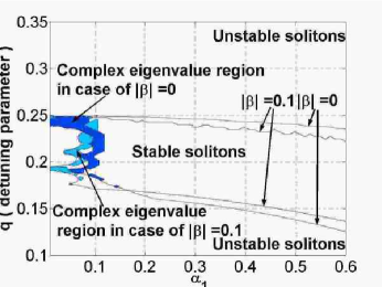
Figure 4: The stability maps for the family of the exact soliton solutions (8) - (11), corresponding to $\beta=0$ and $\alpha_{0}=\left(\alpha_{0}\right)_{\mathrm{exact}}$, see Eq. (12), and for the solitons found numerically for the same $\alpha_{0}$ but $\beta=0.1$. The stability is identified from the computation of the stability eigenvalues (and verified by direct simulations). The shading, bordered by the dashed lines, marks stability sub-regions in which complex eigenvalues were found, while, in the unshaded areas, all the eigenvalues are real.

A similar stability map is shown in Fig. 5 for the same case which was selected above for Fig. 3, i.e., $\alpha_{0}=0.9\left(\alpha_{0}\right)_{\mathrm{exact}}$. Additionally, for both cases $\alpha_{0}=\left(\alpha_{0}\right)_{\mathrm{exact}}$ and $\alpha_{0}=0.9\left(\alpha_{0}\right)_{\mathrm{exact}}$, as well as for another one, $\alpha_{0}=1.1\left(\alpha_{0}\right)_{\mathrm{exact}}$, Fig. 6 shows the area of the stability region as a function of $\beta$, between the two values chosen for the display in Figs. 4 and 5, $\beta=0$ and $\beta=0.1$. Note that two plots in Fig. 6 pertain to exactly the same soliton subfamilies which were included in Figs. 2 and 3. A noticeable observation is that, depending on the value of $\alpha_{0}$, the stability area may both decrease and increase with $\beta$. As concerns the additional case of $\alpha_{0}=1.1\left(\alpha_{0}\right)_{\mathrm{exact}}$, included in Fig. 6, the stability map for it is not very different from that for $\alpha_{0}=\left(\alpha_{0}\right)_{\mathrm{exact}}$, see Fig. 4, therefore it is not displayed here separately.

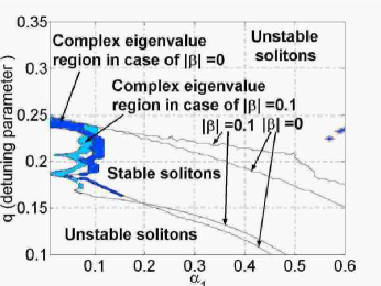
Figure 5: The same as in Fig. 4, but for $\alpha_{0}=0.9\left(\alpha_{0}\right)_{\mathrm{exact}}$.

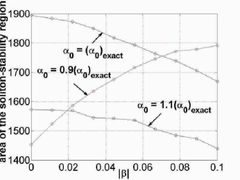
Figure 6: The area of the stability region vs. $\beta$, for three different values of $\alpha_{0}$.

We have also investigated the case when the self-driving coefficient $\beta$ in the FF equation (3) is complex. In this case, the stability maps are not drastically different from the ones displayed above for real $\beta$ (therefore we do not show them here), although the area of the stability region gets somewhat smaller. The area is shown, as a function of $|\beta|$, for two different cases, $\beta=\left(1+i\right)|\beta|/\sqrt{2}$ and $\beta=i|\beta|$, in Fig. 7.

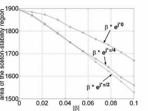
Figure 7: The same as in Fig. 6 for $\alpha_{0}=\left(\alpha_{0}\right)_{\mathrm{exact}}$ and complex $\beta$.

The conclusions concerning the stability of the solitons, which were drawn above on the basis of the stability eigenvalues, where also verified against direct simulations of the full system of Eqs. (3) and (4), performed at a sufficiently dense grid of points covering the predicted stability and instability regions in the system’s phase space. As a result, it has been concluded that all the solitons, which were predicted to be stable, are stable indeed in the direct evolution. The solitons which are expected to be unstable decay to zero under the action of small perturbations or, if the perturbation is stronger, they may rearrange themselves into solitons of a new kind, as described below.

3.3 A bifurcation to the second type of stable solitons

One may observe that the stability areas displayed in Figs. 4 and 5 are located at $q<0.25$. In particular, although we have no analytical proof of the instability of the exact soliton (8) at $q>0.25$, we notice that the value of the mismatch parameter $q=q_{\mathrm{c}}\equiv 0.25$ is a special one for the exact solution, as Eqs. (11) show that the phase $\phi$ vanishes precisely at $q=q_{\mathrm{c}}$.

A stable soliton of a different type can be found at $q>0.25$. This solution, which we will call a type-II soliton, to distinguish it from the one considered above, that we will refer to as type-I, cannot be obtained by the continuation of the exact solution (8). This makes finding the type-II soliton directly from the numerical solution of the stationary version of Eqs. (1) and (2) problematic, as a good initial guess is not available. Nevertheless, it was found, in the region $q>0.25$, in the following way: one can take the numerically exact unstable type-I soliton, and add an arbitrary perturbation to it. A small perturbation initiates decay of the unstable soliton to zero. However, if the perturbation is sufficiently large, the outcome may be spontaneous rearrangement of the pulse into a new stable one, which we identify as the type-II soliton. An example of the unstable type-I soliton (alias separatrix soliton, see below), and its stable type-II counterpart, which is generated from it by a perturbation, is displayed in Fig. 8.

$\begin{array}[]{c@{\hspace{0.5in}}c}\includegraphics[width=180.67499pt]{Fig_34_a.eps}\hfil\hskip 36.135pt&\includegraphics[width=180.67499pt]{Fig_34_b.eps}\\[11.38092pt] \mbox{\bf(a)}\hfil\hskip 36.135pt&\mbox{\bf(b)}\end{array}$

Figure 8: The shape of the unstable type-I (separatrix) and stable type-II solitons in the FH (a) and SH (b) components for for a value of the mismatch parameter exceeding its critical value, $q=0.3>q_{\mathrm{c}}\equiv 0.25$. The other parameters are $\beta=0$, $\alpha_{1}=0.3$, and $\alpha_{0}=\left(\alpha_{0}\right)_{\mathrm{exact}}\approx 0.36$, as per Eq. (12).

The stability map for the type-II solitons was identified, as it was done above for their type-I counterparts in the region $q<0.25$, both by means of the computation of the eigenvalues from the linearized equations, and by means of direct simulations. The resulting map is displayed in Fig. 9. It shows not only the region where the type-II soliton is stable, but also indicates if the perturbation-induced evolution of the unstable type-I solution leads directly to the establishment of the stable type-II soliton, or, instead, transition to an excited state (“breather”) is observed, which then slowly relaxes into the stable type-II soliton. Also shown are regions where the stable soliton does not self-trap; instead, the unstable soliton either decays to zero, or generates a stable delocalized state.

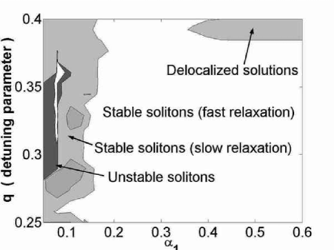
Figure 9: The stability map for the type-II soliton self-trapping from the unstable separatrix (type-I) soliton in the region $q>0.25$. In the regions marked as “fast” and “slow” relaxation, the unstable soliton directly relaxes into the stable one, or does so via formation of a breather with slowly decaying intrinsic oscillations. In the region of “unstable solitons”, the unstable soliton always decays to zero, and in the region of “delocalized solutions”, a spatially periodic state sets in, instead of a stable soliton. The map pertains to $\beta=0$, with $\alpha_{0}$ chosen as per Eq. (12).

The solitons of types I and II are actually connected by a bifurcation. Indeed, the model which supports a stable soliton is a bistable system, as the zero solution is stable too in this case. According to well-known general principles, in a bistable system a separatrix must exist, which is a border between attraction basins of the two stable states. Usually, the role of the separatrix is played by an extra unstable soliton solution, whose amplitude is smaller and width larger than those of the stable soliton (see, e.g., Refs. [24] and [22]). The unstable type-I soliton is such a separatrix in the case of $q>q_{\mathrm{c}}\equiv 0.25$.

The fact that the type-I soliton is stable at $q<q_{\mathrm{c}}$, while no stable soliton of type II was found in that region, implies that a stability-swap bifurcation, involving both solitons, occurs at $q=$ $q_{\mathrm{c}}$. A conjectured bifurcation diagram is schematically depicted in Fig. 10.  

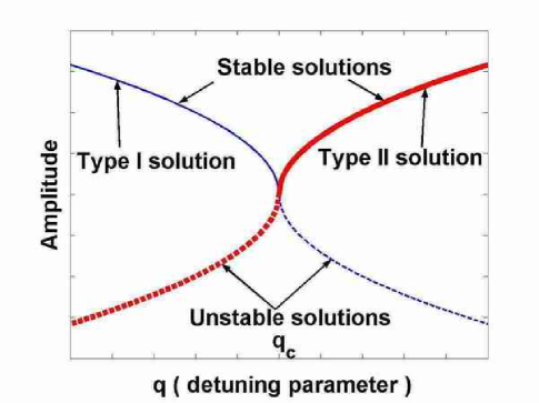
Figure 10: The assumed stability-swap bifurcation between the solitons of types I and II (thin and bold curves) which occurs at the critical value of the mismatch, $q=q_{\mathrm{c}}=0.25$. Stable and unstable solutions are depicted by solid and dashed lines, and the vertical axis refers to the solitons’ amplitudes.

Note that the bifurcation diagram includes an unstable branch in the region of $q<q_{\mathrm{c}}$, which is a conjectured continuation of the type-II solution to $q<q_{\mathrm{c}}$. This branch cannot be readily found from the stationary version of Eqs. (1) and (2), since a good initial guess is not available for it, and it cannot be found in dynamical simulations either, as it is unstable. Thus, while we did not make a strong effort to explicitly find this branch – as, being unstable, it has no direct physical significance – we assume that such a branch exists.

3.4 Stability of solitons in a generalized model

The model based on Eqs. (3) and (4) can be generalized by replacing the evolution and spatial variables $t$ and $x$, respectively, by $z$ and $\tau$:

$$iu_{z}+\frac{1}{2}u_{\tau\tau}+u^{\ast}v = \left(1-i\alpha_{1}\right)u+i\alpha_{0}v^{\ast}+i\beta\left(u^{\ast}\right)^{2},$$

$$iv_{z}+\frac{D}{4}v_{\tau\tau}+\frac{1}{2}u^{2} = \left(2q-i\alpha_{1}\right)v+i\alpha_{0}u^{\ast}.$$ (14)

This model corresponds, instead of the spatial solitons in cavities, to temporal solitons in waveguides. The temporal solitons are localized in the reduced-time variable $\tau$, and propagate along the coordinate $z$. In Eqs. (14), the second derivatives account for the temporal dispersion [rather than diffraction, in the original model (3), (4)], $D$ being a relative SH/FF dispersion coefficient. We have checked that, in this generalization (for instance, with $D=2$, instead of $D=1$), the results for the shape and stability of solitons are very similar to those reported above.

3.5 Investigation of moving solitons

A straightforward extension of the above analysis is to search for moving solitons. Their existence in the present model is not obvious, as the drive terms in Eqs. (3) and (4) (unlike the loss terms) break the Galilean invariance of the equations. Without the drive, the Galilean boost with an arbitrary speed $C$,

$$u\rightarrow u\cdot e^{iCX},v\rightarrow v\cdot e^{2iCX},$$ (15)

transforms any solution $u(x),v(x)$ into a moving one, $u(x-Ct),v(x-Ct)$.

To investigate the possibility of the existence of moving solitons in the present model, we ran systematic numerical experiments, taking the stable soliton solutions in the analytical or numerical form, as found above, and simulating the full system of Eqs. (3) and (4) with the boosted initial conditions (15). The result is that steadily moving solitons are not possible. Instead, a critical value $C_{\mathrm{cr}}$ of the boost parameter $C$ was found, such that the soliton moves for a while but quickly comes to a halt and returns to its initial form, if $C<C_{\mathrm{cr}}$, as shown in Fig. 11. In the opposite case, $C>C_{\mathrm{cr}}$, the soliton always gets destroyed, see an example in Fig. (12).

$\begin{array}[]{c@{\hspace{0.5in}}c}\includegraphics[width=180.67499pt]{Fig_27_a.eps}\hfil\hskip 36.135pt&\includegraphics[width=180.67499pt]{Fig_27_b.eps}\\[11.38092pt] \mbox{\bf(a)}\hfil\hskip 36.135pt&\mbox{\bf(b)}\end{array}$

Figure 11: An example of motion and subsequent stoppage of the boosted soliton (8), in the case of $\alpha_{1}=0.02$, $q=0.245$, $\beta=0$, $\alpha_{0}=\left(\alpha_{0}\right)_{\mathrm{exact}}=2.828$ [see Eq. (12)], and $C=0.3$ (this value of the boost is close to the critical value, which is $C_{\mathrm{cr}}=0.3335$ in the present case). The panels (a) and (b) show the evolution of the pulse’s amplitude profiles in the FF and SH components, respectively.

$\begin{array}[]{c@{\hspace{0.5in}}c}\includegraphics[width=180.67499pt]{Fig_28_a.eps}\hfil\hskip 36.135pt&\includegraphics[width=180.67499pt]{Fig_28_b.eps}\\[11.38092pt] \mbox{\bf(a)}\hfil\hskip 36.135pt&\mbox{\bf(b)}\end{array}$

Figure 12: The same as in Fig. 12, but with the boost parameter $C=0.35$ slightly exceeding the critical value $C_{\mathrm{cr}}$.

The critical boost $C_{\mathrm{cr}}$ depends on values of the model’s parameters. In particular, for the family of the exact solitons taken in the form of Eqs. (8), with $\alpha_{0}$ selected as per Eq. (12), $C_{\mathrm{cr}}$ is shown, as a function of the loss parameter $\alpha_{1}$ at different fixed values of the mismatch $q$, in Fig. (13).

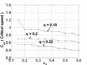
Figure 13: The critical value $C_{\mathrm{cr}}$ of the boost parameter (initial speed), which is defined in Eqs. (15), as a function of $\alpha_{1}$ at fixed values of $q$, for the exact solitons (8) [i.e., with $\beta=0$, and $\alpha_{0}=\left(\alpha_{0}\right)_{\mathrm{exact}}$]. The soliton comes to a halt, or gets destroyed, respectively, in the cases $C<C_{\mathrm{cr}}$ and $C>C_{\mathrm{cr}}$, as shown in Figs. 11 and 12.

The particular mode of the destruction of the boosted soliton in the case of $C>C_{\mathrm{cr}}$ depends on values of the parameters. In particular, instead of the straightforward decay, as in Fig. 12, the soliton may first split into two secondary pulses with different velocities, both of which eventually decay. An example of the latter scenario is displayed in Fig. 14. Also possible are situations in which the soliton does not split, but its FF component decays much faster than the SH one (although the FF and SH loss parameters are equal).

$\begin{array}[]{c@{\hspace{0.5in}}c}\includegraphics[width=180.67499pt]{Fig_24_a.eps}\hfil\hskip 36.135pt&\includegraphics[width=180.67499pt]{Fig_24_b.eps}\\[11.38092pt] \mbox{\bf(a)}\hfil\hskip 36.135pt&\mbox{\bf(b)}\end{array}$

Figure 14: An example of the splitting of the soliton (8) to which an overcritical boost was applied, and subsequent decay of the secondary pulses. In this case, $\alpha_{1}=0.15$, $q=0.2$, $\beta=0$, $\alpha_{0}=\left(\alpha_{0}\right)_{\mathrm{exat}}=\allowbreak 0.25$, the critical value of the boost is $C_{\mathrm{cr}}\approx 0.7$, and the actual value of the boost is $C=0.75$. The panels (a) and (b) show the evolution of the amplitude profiles in the FF and SH components, respectively.

4 Interactions between solitons

Once stable solitons have been found, the next necessary step in the investigation of their fundamental dynamical properties, as well as in the development of potential applications, is the study of interactions between them. To this end, we ran systematic simulations of configurations initially composed of two identical stable solitons with centers placed at a distance $X_{0}$. Note that, unlike the situation in models of the Ginzburg-Landau type (the ones with the intrinsic gain), in models with the parametric gain the phase of each individual soliton is locked to a single value [see Eqs. (8) and (11)], hence the relative phase of the two solitons is not a free parameter, but is equal to zero [25]; for this reason, the solitons always attract each other. The simulations demonstrate that, in all the cases, the attraction gives rise to merger of the two solitons into a single one. If the loss parameter $\alpha_{1}$ is large enough, so that the soliton existing at this value of $\alpha_{1}$ has no complex eigenvalue of small intrinsic perturbations (see Figs. 4 and 5), the resulting single soliton emerges in its stationary form. On the other hand, if $\alpha_{1}$ is small, and the soliton possesses an intrinsic complex eigenvalue, the final soliton appears in an excited (vibrating) state, which then slowly relaxes to the static one. The time necessary for the fusion of the two solitons into one depends on the initial separation $X_{0}$, but the outcome of the interaction does not depend on $X_{0}$.

Below, we illustrate these conclusions by typical examples. In all the cases, we used exact soliton solutions (8) to construct the initial configuration. Simulations of the configuration composed of two solitons of a more general form produced virtually the same results as those displayed below.

If the loss parameter $\alpha_{1}$ is small enough, a pair of exact solitons merge into a pulse which demonstrates nearly persistent intrinsic vibrations, as it was said above and is shown in Fig. 15. Continuing the simulations on a much longer time scale demonstrates that the vibrations slowly fade out, and the pulse relaxes to the static configuration. The latter feature is seen clearer in Fig. 16, which corresponds to a smaller initial separation between the solitons.

$\begin{array}[]{c@{\hspace{0.5in}}c}\includegraphics[width=180.67499pt]{Fig_11a.eps}\hfil\hskip 36.135pt&\includegraphics[width=180.67499pt]{Fig_12a.eps}\\[11.38092pt] \mbox{\bf(a)}\hfil\hskip 36.135pt&\mbox{\bf(b)}\end{array}$

Figure 15: The merger of two solitons, with the initial separation $X_{0}=5.2$ between them, into a pulse with excited internal vibrations, which later slowly relaxes into the stationary soliton. The panels (a) and (b) show the FF and SH components of the field, respectively. The parameters are $q=0.207$, $\alpha_{1}=0.094$, and $\alpha_{0}=\left(\alpha_{0}\right)_{\mathrm{exact}}=0.196$, see Eq. (12).

$\begin{array}[]{c@{\hspace{0.5in}}c}\includegraphics[width=180.67499pt]{Fig_9a.eps}\hfil\hskip 36.135pt&\includegraphics[width=180.67499pt]{Fig_10a.eps}\\[11.38092pt] \mbox{\bf(a)}\hfil\hskip 36.135pt&\mbox{\bf(b)}\end{array}$

Figure 16: The same as in Fig. 15, but for a smaller initial separation between the solitons, $X_{0}=3.6$. In this case, it is obvious that the vibrating pulse, produced by the merger of the two initial solitons, relaxes towards the static soliton.

If $\alpha_{1}$ is larger, so that the soliton does not support intrinsic oscillatory modes, two solitons, even separated by a relatively large distance, fuse into a single soliton which emerges in the stationary state (without intrinsic vibrations), as shown in Fig. 17. The fact that the final soliton is identical to each initial one is obvious from Fig. 18, which compares the initial field configuration in both component and its eventual shape.

$\begin{array}[]{c@{\hspace{0.5in}}c}\includegraphics[width=180.67499pt]{Fig_13a.eps}\hfil\hskip 36.135pt&\includegraphics[width=180.67499pt]{Fig_14a.eps}\\[11.38092pt] \mbox{\bf(a)}\hfil\hskip 36.135pt&\mbox{\bf(b)}\end{array}$

Figure 17: Direct merger of two solitons into a static soliton, in the FF (a) and SH (b) components. The parameters are $q=0.195$, $\alpha_{1}=0.2$, $\alpha_{0}=\left(\alpha_{0}\right)_{\mathrm{exact}}=\allowbreak 0.297$, and the initial separation between the solitons is $X_{0}=5.2$

$\begin{array}[]{c@{\hspace{0.5in}}c}\includegraphics[width=180.67499pt]{Fig_13b.eps}\hfil\hskip 36.135pt&\includegraphics[width=180.67499pt]{Fig_14b.eps}\\[11.38092pt] \mbox{\bf(a)}\hfil\hskip 36.135pt&\mbox{\bf(b)}\end{array}$

Figure 18: The comparison of the initial and final wave-field profiles in the FF (a) and SH (b) components in the same case which is shown in Fig. 17.

5 Conclusion

In this work, we have introduced a model of a lossy second-harmonic-generating ($\chi^{(2)}$) cavity driven by a pump wave at the third harmonic, which gives rise to a new type of driving terms, characterized by the cross-parametric gain. The equation for the fundamental-frequency wave may also contain a quadratic self-driving term, which is generated by the $\chi^{(3)}$ nonlinearity.

Unlike previously studied phase-matched models of $\chi^{(2)}$ cavities driven through down- or upconversion, the present model admits the exact analytical solution for the soliton, at the specially chosen value of the gain parameter. Two general families of soliton solutions were found in a numerical form, one of which is a continuation of the exact analytical solution. At given values of the parameters, one soliton is stable, and one is not. They swap the stability via a bifurcation which occurs at a critical value of the mismatch parameter. Full stability regions of the solitons were identified by means of numerical computation of the corresponding eigenvalues for small perturbations (stability conditions for the zero solution, which is a necessary ingredient of the full conditions for the soliton’s stability, were found in an analytical form). The stability of the solitons was also verified in direct simulations, with the conclusion that the unstable soliton rearranges into the stable one (which may appear in the form of a breather), or into a delocalized state, or decays to zero. Additionally, it was found that steadily moving solitons do not exist in the present model. If the soliton is initially boosted, it either comes to a halt, or, if pushed too hard, gets destroyed (possibly, via splitting into two pulses).

Interactions between initially separated solitons were also investigated by dint of systematic direct simulations. It was found that stable solitons always merge into a single one. In the system with weak loss, the final solitons appears in an excited form (the breather), and then slowly relaxes to the static configuration. If the loss is stronger, the final soliton emerges in the stationary form.

The model introduced in this work can be further investigated in various directions. In particular, a two-dimensional version of this cavity model may be an interesting subject.

References

- [1] A. Gatti, A. Lugiato, L. Spinelli, G. Tissoni, M. Brambilla, P. Di Trapani, F. Pratti, G. L. Oppo, and A. Berzanskis, Chaos, Solitons and Fractals 10, 875 (1999).
- [2] C. O. Weiss, M. Vaupel, K. Staliunas, G. Slekys, and V. B. Taranenko, Appl. Phys. B (Lasers and Opt.) 68, 151 (1999); C. O. Weiss, G. Slekys, V. B. Taranenko, K. Staliunas, and R. Kuszelewicz, V. B. Taranenko, G. Slekys, and C. O. Weiss, Chaos 13, 777 (2003).
- [3] G. L. Oppo, M. Brambilla, and L. A. Lugiato, Phys. Rev. A 49, 2028 (1994).
- [4] S. Trillo and M. Haelterman, Opt. Lett. 23, 1514 (1998).
- [5] C. Etrich, D. Michaelis, and F. Lederer, J. Opt. Soc. Am. B 19, 792 (2002).
- [6] S. Longhi, Phys. Scripta. 56, 611 (1997).
- [7] K. Staliunas and V. J. Sanchez-Morcillo, Opt. Commun. 139, 306 (1997).
- [8] D. V. Skryabin, Phys. Rev. E 60, R3508 (1999).
- [9] D. Michaelis, U. Peschel, C. Etrich, and F. Lederer, IEEE J. Quant. Electr. 39, 255 (2003).
- [10] D. V. Skryabin, A. R. Champneys, and W. J. Firth, Phys. Rev. Lett. 84, 463 (2000).
- [11] V. B. Taranenko, M. Zander, P. Wobben, and C. O. Weiss, Appl. Phys. B (Lasers and Opt.) 69, 337 (1999).
- [12] D. V. Skryabin and A. R. Champneys, Phys. Rev. E 63, 066610 (2001); S. Fedorov, D. Michaelis, U. Peschel, C. Etrich, D. V. Skryabin, N. Rosanov, and F. Lederer, Phys. Rev. E 64, 036610 (2001); A. Barsella, C. Lepers, M. Taki, and M. Tlidi, Opt. Commun. 232, 381 (2004).
- [13] D. V. Skryabin and W. J. Firth, Opt. Lett. 24, 1056 (1999).
- [14] S. Longhi, Opt. Lett. 23, 346 (1998); R. A. Fuerst, M. T. G. Canva, G. I. Stegeman, G. Leo, and G. Assanto, Opt. Quant. Electr. 30, 907 (1998).
- [15] E. Ibragimov, A. A. Struthers, D. J. Kaup, J. D. Khaydarov, and K. D. Singer, Phys. Rev. E 59, 6122 (1999).
- [16] S. C. Rodriguez, J. P. Torres, L. Torner, M. M. Fejer, J. Opt. Soc. Am. 19, 1396 (2002).
- [17] G. L. Oppo, A. J. Scroggie, and W. J. Firth, J. Opt. B Quant. Semicl. Opt. 1, 133 (1999).
- [18] S. Minardi, A. Varanavicus, A. Piskarskas, and P. Di Trapani, Opt. Commun. 224, 301 (2003).
- [19] M. Le Berre, E. Ressayre, and A. Tallet, J. Opt. B - Quant. Semicl. Opt. 2, 347(2000).
- [20] Y. S. Kivshar, T. J. Alexander, and S. Saltiel, Opt. Lett. 24, 759 (1999).
- [21] G. J. Valcarcel, E. Roldan, and K. Staliunas, Opt. Commun. 181, 207(2000).
- [22] I. V. Barashenkov, M. M. Bogdan, and V. I. Korobov, Europhys. Lett. 15, 113 (1991).
- [23] L.-C. Crasovan, B. A. Malomed, D. Mihalache, D. Mazilu, and F. Lederer, Phys. Rev. E 62, 1322 (2000).
- [24] B.A. Malomed, Physica D 29, 155 (1987).
- [25] D. Cai, A. R. Bishop, N. Grønbech-Jensen, and B.A. Malomed, Phys. Rev. E 49, 1677 (1994).