On Optimal Canonical Variables in the Theory of Ideal Fluid with Free Surface

Abstract

Dynamics of ideal fluid with free surface can be effectively solved by perturbing the Hamiltonian in weak nonlinearity limit. However it is shown that perturbation theory, which includes third and fourth order terms in the Hamiltonian, results in the ill-posed equations because of short wavelength instability. To fix that problem we introduce the canonical Hamiltonian transform from original physical variables to new variables for which instability is absent.

Keywords: Surface waves; Ill-posedness; Canonical transform

I Introduction

The Euler equations describing dynamics of ideal fluid with free surface is a Hamiltonian system, which is especially simple if the fluid motion is potential, ${\bf v}=\nabla\Phi$, where ${\bf v}$ is the fluid’s velocity and $\Psi$ is the velocity potential. In this case Zakharov1966 ; Zakharov1968 ; ZakharovEurJ1999 the Euler equations can be presented in the form:

$$\frac{\partial\eta}{\partial t}=\frac{\delta H}{\delta\Psi},\quad\frac{\partial\Psi}{\partial t}=-\frac{\delta H}{\delta\eta}.$$ (1)

Here $z=\eta({\bf r})$ is the shape of surface, $z$ is vertical coordinate and ${\bf r}=(x,y)$ are horizontal coordinates, $\Psi\equiv\Phi\big{|}_{z=\eta}$ is the velocity potential on the surface. The Hamiltonian $H$ coincides with the total (potential and kinetic) energy of fluid. The Hamiltonian cannot be expressed in a closed form as a function of surface variables $\eta,\,\Psi$, but it can be presented by the infinite series in powers of surface steepness $|\nabla\eta|$:

$$H=H_{0}+H_{1}+H_{2}+\ldots.$$ (2)

Here $H_{0},\ H_{1},\ H_{2}$ are quadratic, cubic and quartic terms, respectively. Equations $(\ref{hameq1}),(\ref{hamserdef})$ are widely used now for numerical simulation of the fluid dynamics CraigWorfolk1995 ; DyachenkoKorotkevichZakharovJETPLett2003a ; DyachenkoKorotkevichZakharovJETPLett2003b ; DyachenkoKorotkevichZakharovPRL2004 ; OnoratoZakharovPRL2002 ; PushkarevEurJMech1996 ; PushkarevZakharovPRL1996 ; PushkarevZakharovPhysD2000 ; TanakaJFM2001 ; ZakharovDyachenkoVasilyevEurJ2002 ; Krasitskii1990 . These simulations are performing by the use of the spectral code, at the moment a typical grid is $512\times 512$ harmonics.

Canonical variables are used also for analytical study of the surface dynamics in the limit of small steepness. It was shown KuznetsovSpektorZakharov1993 ; KuznetsovSpektorZakharov1994 ; DyachenkoZakharovKuznetsov1996 that the simplest truncation of the series $(\ref{hamserdef})$, namely

$$H=H_{0}+H_{1},$$ (3)

leads to completely integrable model - complex Hopf equation. In framework of this approach one can develop the self-consistent theory of singularity formation in absence of gravity and capillarity for two dimensions (one vertical coordinate $z$ and one horizontal coordinate $x$).

However, use of canonical variables $\eta,\,\Psi$ has a weak point, which becomes clear, if we concentrate our attention on the complex Hopf equation,

$$\frac{\partial\Pi}{\partial t}=-\frac{1}{2}\Big{(}\frac{\partial\Pi}{\partial x}\Big{)}^{2},$$ (4)

which comes from Eqs. $(\ref{hameq1}),(\ref{htrunc1})$. Here

$$\Psi=Re(\Pi)$$ (5)

and $\Pi$ is the analytic function of the complex variable $x$ in a strip $-h\leq Im(x)\leq 0$, $h$ is the depth of the fluid. The weak point is that Eq. $(\ref{hopfp})$ is ill-posed. A general complex solution of this equation is unstable with respect to grow of small short-wave perturbations. The same statement is correct with respect to more exact fourth order Hamiltonian

$$H=H_{0}+H_{1}+H_{2},$$ (6)

which is used in most numerical experiments. These experiments are easy becomes unstable: to arrest instability one should include into equations strong artificial damping at high wave numbers. Even in presence of such damping one can simulate only waves of a relatively small steepness (not more than $0.15$).

In this Article we show that these difficulties can be fixed by a proper canonical transformation to another canonical variables. It is remarkable, but the property of nonlinear wave equation to be well- or ill-posed is not invariant with respect to choice of the variables.

In the present Article we demonstrate that there are new canonical variables such that the Eqs. $(\ref{hameq1}),(\ref{hamfourth})$ are well-posed if we consider the nonlinearity up to the fourth order in the Hamiltonian. We call these variables “optimal canonical variables”. We demonstrate in the present Article that the choice of the optimal canonical variables is unique provided we additionally require the Hamiltonian system to be free of short wavelength instability for largest possible steepness of the surface, i.e. for the largest possible nonlinearity. We conjecture that optimal canonical variables allow simulation with higher steepness compare with standard variables $\Psi,\,\eta.$ We can also formulate a conjecture that the optimal canonical variables exist in all orders of nonlinearity.

II Basic equations and the Hamiltonian formalizm

Consider the dynamics of an incompressible ideal fluid with free surface and constant depth. Fluid occupies the region

$$-h<z<\eta({\bf r}),\quad{\bf r}=(x,y),$$ (7)

where $(x,y)$ are the horizontal coordinates and $z$ is the vertical coordinate.

Viscosity is assumed to be absent and the fluid’s velocity ${\bf v}$ is potential one,

$${\bf v}=\nabla\Phi,$$ (8)

where $\Phi$ is the velocity potential. Incompressibility condition,

$$\nabla\cdot{\bf v}=0,$$ (9)

results in the Laplace Eq.

$$\triangle\Phi=0.$$ (10)

The potential $\Phi$ satisfies also the Bernoulli equation:

$$\Phi_{t}+\frac{1}{2}\big{(}\nabla\Phi\big{)}^{2}+p+gz=0,$$ (11)

where $p$ is the pressure, $g$ is the acceleration of gravity, and we set density of fluid to unity.

There are two types of boundary conditions at free surface for Eqs. $(\ref{lapl1}),(\ref{bernoulli})$. First is the kinematic boundary condition

$$\frac{\partial\eta}{\partial t}=\Big{(}\Phi_{z}-\nabla\eta\cdot\nabla\Phi\Big{)}\Big{|}_{z=\eta}=v_{n}\sqrt{1+(\nabla\eta)^{2}},$$ (12)

where $v_{n}={\bf n}\cdot\nabla\Phi$ is the normal component of fluid’s velocity at free surface, and ${\bf n}=(-\nabla\eta,1)\big{[}1+(\nabla\eta)^{2}\big{]}^{-1/2}$ is the interface normal vector.

Second is the dynamic boundary condition at free surface

$$p\big{|}_{z=\eta}=\sigma\nabla\cdot\frac{\nabla\eta}{\sqrt{1+(\nabla\eta)^{2}}},$$ (13)

where $\sigma$ is the surface tension coefficient which determines the jump of the pressure at free surface from zero value outside of the fluid to $p\big{|}_{z=\eta}$ value inside fluid.

Boundary condition at the bottom is

$$\Phi_{z}|_{z=-h}=0.$$ (14)

Eqs. $(\ref{lapl1})-(\ref{boundarybottom1})$ form a closed set of equations to determine the dynamics of free surface.

The total energy, $H$, of the fluid consists of the kinetic energy, $T,$ and the potential energy, $U$:

$$H=T+U,$$ (15)

$$T=\frac{1}{2}\int d{\bf r}\int^{\eta}_{-h}\big{(}\nabla\Phi\big{)}^{2}dz,$$ (16)

$$U=\frac{1}{2}g\int\eta^{2}\,d{\bf r}+\sigma\int\Big{[}\sqrt{1+\big{(}\nabla\eta\big{)}^{2}}-1\Big{]}d{\bf r}.$$ (17)

It is convenient to introduce the value of the velocity potential at interface as

$$\Phi\big{|}_{z=\eta}\equiv\Psi({\bf r},t).$$ (18)

It was shown in Ref. Zakharov1968 that the free surface problem $(\ref{lapl1})-(\ref{boundarybottom1})$ can be written in the Hamiltonian form $(\ref{hameq1})$, with the Hamiltonian $H$ defined in $(\ref{hamdef})$.

Fourier transform,

$$\Psi_{{\bf k}}=\frac{1}{2\pi}\int\exp(-i{\bf k}\cdot{\bf r})\Psi({\bf r})d{\bf r},$$ (19)

is the canonical transform which conserves the Hamiltonian structure and Eqs. $(\ref{hameq1})$ take the following form:

$$\frac{\partial\eta_{\bf k}}{\partial t}=\frac{\delta H}{\delta\Psi_{-{\bf k}}},\quad\frac{\partial\Psi_{\bf k}}{\partial t}=-\frac{\delta H}{\delta\eta_{-{\bf k}}},\quad\eta_{\bf k}^{*}=\eta_{-{\bf k}},\quad\Psi_{\bf k}^{*}=\Psi_{-{\bf k}}.$$ (20)

III Weak nonlinearity

If a typical slope of free surface is small, $|\nabla\eta|\ll 1$, the Hamiltonian $H$ can be series expanded (see Eq. $(\ref{hamserdef})$) in powers of steepness $|\nabla\eta|$ which gives Zakharov1968 ; ZakharovEurJ1999 :

$$H_{0}=\frac{1}{2}\int\Big{\{}A_{k}|\Psi_{\bf k}|^{2}+B_{k}|\eta_{\bf k}|^{2}\Big{\}}d{\bf k},$$

$$A_{k}=k\tanh(kh),\ B_{k}=g+\sigma k^{2},\ k=|{\bf k}|,$$ (21)

$$H_{1}=\frac{1}{4\pi}\int L^{(1)}_{{\bf k}_{1},{\bf k}_{2}}\Psi_{{\bf k}_{1}}\Psi_{{\bf k}_{2}}\eta_{{\bf k}_{3}}\delta({\bf k}_{1}+{\bf k}_{2}+{\bf k}_{3})d{\bf k}_{1}d{\bf k}_{2}d{\bf k}_{3}$$ (22)

$$H_{2}=\frac{1}{2(2\pi)^{2}}\int\Big{[}L^{(2)}_{{\bf k}_{1},{\bf k}_{2},{\bf k}_{3},{\bf k}_{4}}\Psi_{{\bf k}_{1}}\Psi_{{\bf k}_{2}}-\frac{\sigma}{4}({\bf k}_{1}\cdot{\bf k}_{2})({\bf k}_{3}\cdot{\bf k}_{4})\eta_{{\bf k}_{1}}\eta_{{\bf k}_{2}}\Big{]}$$

$$\times\eta_{{\bf k}_{3}}\eta_{{\bf k}_{4}}\delta({\bf k}_{1}+{\bf k}_{2}+{\bf k}_{3}+{\bf k}_{4})d{\bf k}_{1}d{\bf k}_{2}d{\bf k}_{3}d{\bf k}_{4},$$ (23)

where matrix elements are given by

$$L^{(1)}_{{\bf k}_{1},{\bf k}_{2}}=-{\bf k}_{1}\cdot{\bf k}_{2}-A_{1}A_{2},$$

$$L^{(2)}_{{\bf k}_{1},{\bf k}_{2},{\bf k}_{3},{\bf k}_{4}}=\frac{1}{4}A_{1}A_{2}\Big{(}A_{1+3}+A_{2+3}+A_{1+4}+A_{2+4}\Big{)}$$

$$-\frac{1}{2}(k_{1}^{2}A_{2}+k_{2}^{2}A_{1}),\quad A_{j}\equiv A_{k_{j}},\ A_{j+l}\equiv A_{{\bf k}_{j}+{\bf k}_{l}}.$$ (24)

The corresponding dynamical equations follow from $(\ref{hameq1}),(\ref{hamfourth}),(\ref{ham0}),(\ref{ham1}),(\ref{ham2}):$

$$\frac{\partial\Psi}{\partial t}=-g\eta+\sigma\triangle\eta+\frac{1}{2}\Big{[}\big{(}\hat{A}\Psi\big{)}^{2}-\big{(}\nabla\Psi\big{)}^{2}\Big{]}-(\hat{A}\Psi)\hat{A}\big{[}\eta(\hat{A}\Psi)\big{]}$$

$$-(\triangle\Psi)(\hat{A}\Psi)\eta-\frac{\sigma}{2}\nabla\cdot\Big{[}\nabla\eta(\nabla\eta\cdot\nabla\eta)\Big{]},$$

$$\frac{\partial\eta}{\partial t}=\hat{A}\Psi-\nabla\cdot\big{[}(\nabla\Psi)\eta\big{]}-\hat{A}\big{[}\eta\hat{A}\Psi\big{]}+\hat{A}\Big{\{}\eta\hat{A}\big{[}\eta\hat{A}\Psi\big{]}\Big{\}}$$

$$+\frac{1}{2}\triangle\big{[}\eta^{2}\hat{A}\Psi\big{]}+\frac{1}{2}\hat{A}\big{[}\eta^{2}\triangle\Psi\big{]},$$ (25)

where $\hat{A}$ is the linear integral operator which corresponds to multiplication on $k\tanh(kh)$ in Fourier space. For two dimensional flow, $\Psi(x,y)=\Psi(x),\,\eta(x,y)=\eta(x)$, this operator is given by

$$\hat{A}=-\frac{\partial}{\partial x}\hat{R}$$ (26)

$$\hat{R}f(x)=\frac{1}{2h}P.V.\int^{+\infty}_{-\infty}\frac{f(x^{\prime})}{\sinh\big{[}(x^{\prime}-x)\pi/(2h)\big{]}}\ dx^{\prime}$$ (27)

where $P.V.$ means Cauchy principal value of integral. In the limiting case of infinitely deep water, $h\to\infty$, the operator $\hat{A}$ turns into the operator $\hat{k}$

$$\lim_{h\to\infty}\hat{A}=\hat{k}$$ (28)

which corresponds to multiplication on $|{\bf k}|$ in Fourier space while the operator $\hat{R}$ for two-dimentsional flow turns into the Hilbert transform:

$$\lim_{h\to\infty}\hat{R}=\hat{H},\quad\hat{H}f(x)=\frac{1}{\pi}P.V.\int^{+\infty}_{-\infty}\frac{f(x^{\prime})}{x^{\prime}-x}dx^{\prime}.$$ (29)

$\hat{H}$ can be also interpreted as a Fourier transform of $i\,\mbox{sign}(k)$.

If one neglects gravity and surface tension, $g=0,\,\sigma=0,$ then Eqs. $(\ref{hameq1}),(\ref{hamserdef})$, at leading order over small parameter $|\nabla\eta|$, result inKuznetsovSpektorZakharov1994 ; KuznetsovSpektorZakharov1993 ; DyachenkoZakharovKuznetsov1996

$$\frac{\partial\eta}{\partial t}=\hat{A}\Psi,$$ (30a)

$$\frac{\partial\Psi}{\partial t}=\frac{1}{2}\Big{[}\big{(}\hat{A}\Psi\big{)}^{2}-\big{(}\nabla\Psi\big{)}^{2}\Big{]}.$$ (30b)

Remarkable feature of Eqs. $(\ref{etaeq0}),(\ref{psieq0})$ is that the second Eq. $(\ref{psieq0})$ does not depend on $\eta$ thus one can first solve $(\ref{psieq0})$ and then find $\eta$ from Eq. $(\ref{etaeq0})$. Substitution $\Pi\equiv\Psi+i\hat{R}\Psi$ into Eq. $(\ref{psieq0})$ results in the complex Hopf Eq. $(\ref{hopfp})$ for two-dimensional flow DyachenkoZakharovKuznetsov1996 which is completely integrable.

Both Eqs. $(\ref{psieq0})$ and $(\ref{hopfp})$ are ill-posed because they have short wavelength instability which is determined as follows: we can analyze Eq. $(\ref{psieq0})$ and take $\Psi$ in the form

$$\Psi=\Psi_{0}+\Big{(}\Psi_{1}e^{i{\bf k}\cdot{\bf r}+\nu t}+c.c.\Big{)},$$ (31)

where $\Psi_{0}({\bf r},t)$ is a solution of Eq. $(\ref{psieq0})$, $\Psi_{1}$ is the amplitude of small perturbation, and c.c. means complex conjugation. Then, in the limit $|{\bf k}|\to\infty$, $\Psi_{0}$ evolves very slow in space compare to $e^{i{\bf k}\cdot{\bf r}+\nu t}$ and we get the dispersion relation for small perturbations:

$$\nu=A_{k}\hat{A}\Psi_{0}-i{\bf k}\cdot\nabla\Psi_{0}$$ (32)

which describes instability for $Re(\nu)=A_{k}\hat{A}\Psi_{0}>0$. For general initial condition such instability region always exists. The instability growth rate, $Re(\nu)$ grows as $|{\bf k}|$ increases.

IV Short wavelength stability analysis of the fourth-order Hamiltonian

To study linear stability of the Hamiltonian system in respect to short wavelength perturbations one can set

$$\eta_{\bf k}=\eta_{0\,{\bf k}}+\delta\eta_{\bf k},$$

$$\Psi_{\bf k}=\Psi_{0\,{\bf k}}+\delta\Psi_{\bf k},$$ (33)

where $\eta_{0\,{\bf k}},\,\Psi_{0\,{\bf k}}$ are solutions of Eqs. $(\ref{hameq1}),(\ref{hamfourth})$ and $\delta\eta_{{\bf k}},\,\delta\psi_{{\bf k}}$ are short wavelength perturbations localized around wave vector ${\bf k},|{\bf k}|\gg q$, $q$ is a typical wavenumber for $\eta_{0\,{\bf k}},\,\Psi_{0\,{\bf k}}$.

If we take into account contribution to the fourth-order Hamiltonan up to second order in amplitude of perturbations $\delta\eta_{{\bf k}},\,\delta\Psi_{{\bf k}}$ we get the following general form of the perturbed Hamiltonian:

$$\delta H_{0}=\frac{1}{2}\int\tilde{A}_{\bf k}|\delta\Psi_{\bf k}|^{2}d{\bf k}+\frac{1}{2}\int\tilde{B}_{\bf k}|\delta\eta_{\bf k}|^{2}d{\bf k}+\int(F_{\bf k}+iG_{\bf k})\delta\Psi_{\bf k}\delta\eta_{-{\bf k}}d{\bf k},$$

$$\tilde{A}_{\bf k}=\tilde{A}_{-{\bf k}},\ \tilde{B}_{\bf k}=\tilde{B}_{-{\bf k}},\ F_{\bf k}=F_{-{\bf k}},\ G_{\bf k}=-G_{-{\bf k}},$$ (34)

where $\tilde{A}_{\bf k},\ \tilde{B}_{-{\bf k}},\ F_{\bf k},\ G_{\bf k}$ are real and depend on $\eta_{0\,{\bf k}},\,\Psi_{0\,{\bf k}}$. Here we disregard linear contribution to $\delta H_{0}$ because it has no effect on linear stability analysis.

It follows from Eqs. $(\ref{hamfoureq1}),(\ref{H2lin})$ that equations of motion take the following form:

$$\frac{\partial\delta\eta_{\bf k}}{\partial t}=\tilde{A}_{\bf k}\delta\Psi_{\bf k}+(F_{\bf k}-iG_{\bf k})\eta_{\bf k},$$

$$\frac{\partial\delta\Psi_{\bf k}}{\partial t}=-\tilde{B}_{\bf k}\delta\eta_{\bf k}-(F_{\bf k}+iG_{\bf k})\Psi_{\bf k}.$$ (35)

An assumption of exponential dependence on time,

$$\delta\eta_{\bf k}\sim e^{\nu_{\bf k}t},\ \delta\Psi_{\bf k}\sim e^{\nu_{\bf k}t},$$ (36)

gives a dispersion relation

$$\nu_{\bf k}=-iG_{\bf k}\pm\sqrt{F_{\bf k}^{2}-\tilde{A}_{\bf k}\tilde{B}_{\bf k}}$$ (37)

which describes instability provided $F_{\bf k}^{2}-\tilde{A}_{\bf k}\tilde{B}_{\bf k}>0.$

V Ill-posedness of the fourth-order Hamiltonian

Consider now a general case of nonzero $g$ and $\sigma$ and take into account all terms in the Hamiltonian up to forth order, i.e. consider full Eqs. $(\ref{dynamics1})$. At the leading order over steepness $\Theta$ and wavenumber $k$ we obtain:

$$\tilde{A}_{\bf k}=A_{k}+(k^{2}-A_{k}^{2})\eta_{0}-A_{k}(k^{2}-A_{k}^{2})\eta_{0}^{2}+O(k\Theta^{2}),$$

$$\tilde{B}_{\bf k}=B_{k}+A_{k}(\hat{A}\Psi_{0})^{2}+O(k^{0}v_{0}^{2}l_{0}^{-1}),$$

$$F_{\bf k}=-A_{k}\hat{A}\Psi_{0}-(k^{2}-A_{k}^{2})(\hat{A}\Psi_{0})\eta_{0}+A_{k}\big{(}\hat{A}\big{[}\eta_{0}\hat{A}\Psi_{0}\big{]}+\eta_{0}\nabla^{2}\Psi_{0}\big{)}$$

$$+O(k^{0}v_{0}l_{0}^{-1}),$$

$$G_{\bf k}={\bf k}\cdot\nabla\Psi_{0}+O(kv_{0}\Theta),$$ (38)

where $\eta_{0}=\frac{1}{2\pi}\int\eta_{\bf k}d{\bf k},\ \Psi_{0}=\frac{1}{2\pi}\int\Psi_{\bf k}d{\bf k},$ and the steepness is defined as $\Theta\sim|\nabla\eta_{0}|$. We introduced here the typical value of fluid velocity, $v_{0}\sim|\nabla\Psi_{0}|$ and the typical scale, $l_{0}$, of variation of $v_{0}$ and $\eta_{0}:$ $\Theta\sim\eta_{0}/l_{0},\ |\nabla v_{0}|\sim v_{0}/l_{0}.$

Eqs. $(\ref{nuk2}),(\ref{AB2})$ give instability growth rate. We consider particular cases. If $\sigma\neq 0$ then in the limit $|{\bf k}|\to\infty$, we have

$$\nu_{\bf k}=\pm i\sqrt{\sigma k^{3}},$$ (39)

i.e. instability is absent. In derivation of Eq. $(\ref{nuksigma2})$ we used exponential smallness of expression $k^{2}-A_{k}^{2}=k^{2}/(\cosh{kh})^{2}\simeq 4k^{2}\exp(-kh)\ll 4k^{2}$ because limit $|{\bf k}|\to\infty$ implies $kh\gg 1$. Thus finite $\sigma$ makes problem $(\ref{hamfoureq1}),(\ref{ham0})-(\ref{ham2})$ well-posed.

Note that for finite depth $A_{k}<k$ we could still have instability at finite range of wavenumbers $kh\sim 1$. In that case $k\eta_{0}\sim\eta_{0}/h\ll 1$ because a typical variation of surface elevation, $\eta_{0}$, should be small to allow weak nonlinearity approximation used throughout this Article. Because $k\eta_{0}\ll 1$, Eqs. $(\ref{nuk2}),(\ref{AB2})$ are reduced to

$$\nu_{\bf k}=-i{\bf k}\cdot\nabla\Psi_{0}\pm A_{k}^{1/2}\big{[}-B_{k}+2(k^{2}-A_{k}^{2})(\hat{A}\Psi_{0})^{2}\eta_{0}\big{]}^{1/2},\quad kh\sim 1,$$ (40)

which gives instability provided

$$B_{k}<2(k^{2}-A_{k}^{2})(\hat{A}\Psi_{0})^{2}\eta_{0},\quad kh\sim 1.$$ (41)

E.g. instability occurs for $g=\sigma=0$:

$$\nu_{\bf k}=-i{\bf k}\cdot\nabla\Psi_{0}\pm k(\hat{A}\Psi_{0})\eta_{0}\sqrt{k^{2}-A_{k}^{2}},\quad kh\sim 1.$$ (42)

We can estimate inequality $(\ref{instabcond01})$ as

$$(g+\frac{\sigma}{h^{2}})\lesssim\frac{v_{0}^{2}\eta_{0}}{h^{2}},$$ (43)

where $v_{0}\sim|\nabla\Psi_{0}|$ is the typical velocity of fluid.

It follows from $(\ref{instabestimate01})$ that instability occurs for large values of $v_{0}$ (because $\eta_{0}$ is small). If gravity dominates, $g>\sigma/h^{2}$, then $(\ref{instabestimate01})$ gives $gh/v_{0}^{2}\lesssim\eta_{0}/h$ but weak nonlinearity approximation implies that $\eta_{0}/h\ll 1$ which indicates that the kinetic energy strongly exceed the potential energy. Fluid has enough kinetic energy to easily move upward at distance $\sim h$. As a result, at later stage of evolution weak nonlinearity approximation is violated and surface is strongly perturbed at scales $\sim h$.

If capillarity dominates, $g<\sigma/h^{2},$ inequality $(\ref{instabestimate01})$ gives $\sigma/(v_{0}^{2}\eta_{0})\lesssim 1$ and the kinetic energy again strongly exceed the potential energy. Assume now that, because of instability for $kh\sim 1$, at later time of evolution the potential energy will be of the same order as the kinetic energy, namely, $\eta_{0}v_{0}^{2}\sim\sigma\Theta^{2},\ \Theta\sim|\nabla\eta|$. Then $\sigma/(v_{0}^{2}\eta_{0})\lesssim 1$ results in inequality $\Theta\gtrsim 1$ which again violates weak nonlinearity approximation. Thus for arbitrary relations between $g$ and $\sigma/h^{2}$, and for $kh\sim 1$, the instability is possible for strong enough velocity of fluid and this instability results in violation of weak nonlinearity approximation in course of fluid evolution. In that sense there is no surprise that for large velocity there is an instability for $kh\sim 1$. This instability is purely physical which leaves problem well-posed.

Outside capillary scale we can set $\sigma=0$ and get from Eqs. $(\ref{nuk2}),(\ref{AB2})$ that zero capillarity makes Eqs. $(\ref{dynamics1})$ ill-posed for $k\to\infty:$

$$\nu_{\bf k}=-i{\bf k}\cdot\nabla\Psi_{0}\pm 2^{1/2}(\hat{A}\Psi_{0})^{1/2}k\big{(}\hat{A}\big{[}\eta_{0}\hat{A}\Psi_{0}\big{]}+\eta_{0}\nabla^{2}\Psi_{0}\big{)}^{1/2}$$

$$\sim-i{\bf k}\cdot\nabla\Psi_{0}\pm kv_{0}\Theta^{1/2}.$$ (44)

An expression $\hat{A}\Psi_{0}\Big{(}\hat{A}\big{[}\eta_{0}\hat{A}\Psi_{0}\big{]}+\eta_{0}\nabla^{2}\Psi_{0}\Big{)}$ in Eq. $(\ref{nukhzerosigma2})$ is not sign-definite which results in instability of the system $(\ref{hamfoureq1}),(\ref{ham0})-(\ref{ham2})$. It means that the fourth order Hamiltonian does not prevent short-wavelength instability but makes instability weaker by the small factor $\Theta^{1/2}$ compare with instability of the third-order Hamiltonian (compare Eqs. $(\ref{nukhzerosigma2})$ and $(\ref{nu01})$). Instability $(\ref{nukhzerosigma2})$ has been observed numerically Dyachenkounpublished . We conclude that full fourth order system $(\ref{hamfoureq1}),(\ref{ham0})-(\ref{ham2})$ is ill-posed for zero capillarity, $\sigma=0.$

Ill-posedness of Eqs. $(\ref{hamfoureq1}),(\ref{ham0})-(\ref{ham2})$ can be also interpreted as violation of perturbation expansion $(\ref{hamserdef})$ for $k\to\infty.$ Namely, short wavelength contribution to the quadratic Hamiltonian $(\ref{H2lin}),(\ref{AB2})$ is not small compare with the other terms in the Hamiltonian $(\ref{ham0})-(\ref{ham2})$ provided $k\eta_{0}\gtrsim 1.$

Ill-posedness makes Eqs. $(\ref{hamfoureq1}),(\ref{ham0})-(\ref{ham2})$ (or, equivalently, Eqs. $(\ref{dynamics1})$) difficult for simulations. There a few ways to cope with that problem. One way is to resolve all scales down to capillary scales which is extremely costly numerically. E.g., if we want to study water waves in gravitation region (scale of meters and larger), we would have to simultaneously resolve capillary scale $\sim 1cm$. Other way is to introduce artificial damping for short wavelengths, i.e. to replace Eqs. $(\ref{hamfoureq1})$ by

$$\frac{\partial\eta_{\bf k}}{\partial t}=\frac{\delta H}{\delta\Psi_{-{\bf k}}}+\gamma_{1}(k)\eta_{\bf k},\quad\frac{\partial\Psi_{\bf k}}{\partial t}=-\frac{\delta H}{\delta\eta_{-{\bf k}}}+\gamma_{2}(k)\Psi_{\bf k},$$ (45)

where functions $\gamma_{1}(k),\,\gamma_{2}(k)$ are zero for small and intermediate values of $k$ but they tend to $-\infty$ for $k\to\infty$. Also it is possible to introduce finite viscosity of the fluid. However in that case we would have to resolve very small scales and, in addition, the Hamiltonian is not conserved for finite viscosity so that we can not use the Hamiltonian formalism.

In this Paper we use another way which is to completely remove short wavelength instabilities and make problem well-posed by appropriate canonical transform from variables $\eta,\,\Psi$ to new canonical variables $\xi,\,R.$

VI Canonical transform

Canonical transform from variables $\Psi,\eta$ to new variables $R,\xi$ is determined by a generating functional $S:$

$$S=\int R_{\bf k}\eta_{-{\bf k}}d{\bf k}+\frac{1}{8\pi}\int A_{3}\eta_{{\bf k}_{1}}\eta_{{\bf k}_{2}}R_{{\bf k}_{3}}\delta({\bf k}_{1}+{\bf k}_{2}+{\bf k}_{3})d{\bf k}_{1}d{\bf k}_{2}d{\bf k}_{3}$$

$$+\frac{1}{4(2\pi)^{2}}\int V_{{\bf k}_{1},{\bf k}_{2},{\bf k}_{3},{\bf k}_{4}}R_{{\bf k}_{1}}\eta_{{\bf k}_{2}}\eta_{{\bf k}_{3}}\eta_{{\bf k}_{4}}\delta({\bf k}_{1}+{\bf k}_{2}+{\bf k}_{3}+{\bf k}_{4})d{\bf k}_{1}d{\bf k}_{2}d{\bf k}_{3}d{\bf k}_{4},$$ (46)

$$\Psi_{\bf k}=\frac{\delta S}{\delta\eta_{-{\bf k}}}=R_{\bf k}+\frac{1}{4\pi}\int A_{1}R_{{\bf k}_{1}}\eta_{{\bf k}_{2}}\delta({\bf k}_{1}+{\bf k}_{2}-{\bf k})d{\bf k}_{1}d{\bf k}_{2}$$

$$+\frac{3}{4(2\pi)^{2}}\int V_{{\bf k}_{1},{\bf k}_{2},{\bf k}_{3},-{\bf k}}R_{{\bf k}_{1}}\eta_{{\bf k}_{2}}\eta_{{\bf k}_{3}}\delta({\bf k}_{1}+{\bf k}_{2}+{\bf k}_{3}-{\bf k})d{\bf k}_{1}d{\bf k}_{2}d{\bf k}_{3},$$ (47a)

$$\xi_{\bf k}=\frac{\delta S}{\delta R_{-{\bf k}}}=\eta_{\bf k}+\frac{1}{8\pi}\int A_{k}\eta_{{\bf k}_{1}}\eta_{{\bf k}_{2}}\delta({\bf k}_{1}+{\bf k}_{2}-{\bf k})d{\bf k}_{1}d{\bf k}_{2}$$

$$+\frac{1}{4(2\pi)^{2}}\int V_{-{\bf k},{\bf k}_{2},{\bf k}_{3},{\bf k}_{4}}\eta_{{\bf k}_{2}}\eta_{{\bf k}_{3}}\eta_{{\bf k}_{4}}\delta({\bf k}_{2}+{\bf k}_{3}+{\bf k}_{4}-{\bf k})d{\bf k}_{2}d{\bf k}_{3}d{\bf k}_{4},$$ (47b)

where $V_{{\bf k}_{1},{\bf k}_{2},{\bf k}_{3},{\bf k}_{4}}$ is the symmetric function of ${\bf k}_{2},{\bf k}_{3},{\bf k}_{4}.$ This is the most general form of canonical transform up to terms of the fourth order. The only condition which we use here is that $S$ is chosen to be linear functional of $R$ to preserve the quadratic dependence of the Hamiltonian on canonical momentum $R$.

The quantity $\eta$ can be found from Eq. $(\ref{xidef})$ as the functional of $\xi$ by iterations (here and below we take into account only corrections up to the fourth order in the Hamiltonian):

$$\eta_{\bf k}=\xi_{\bf k}-\frac{1}{8\pi}\int A_{k}\xi_{{\bf k}_{1}}\xi_{{\bf k}_{2}}\delta({\bf k}_{1}+{\bf k}_{2}-{\bf k})d{\bf k}_{1}d{\bf k}_{2}+\frac{1}{8(2\pi)^{2}}$$

$$\times\int\Big{[}A_{k}A_{1+2}-2V_{-{\bf k},{\bf k}_{1},{\bf k}_{2},{\bf k}_{3}}\Big{]}\xi_{{\bf k}_{1}}\xi_{{\bf k}_{2}}\xi_{{\bf k}_{3}}\delta({\bf k}_{1}+{\bf k}_{2}+{\bf k}_{3}-{\bf k})d{\bf k}_{1}d{\bf k}_{2}d{\bf k}_{3},$$ (48)

Eqs. $(\ref{psidef}),(\ref{etaeq1})$ give:

$$\Psi_{\bf k}=R_{\bf k}+\frac{1}{4\pi}\int A_{1}R_{{\bf k}_{1}}\xi_{{\bf k}_{2}}\delta({\bf k}_{1}+{\bf k}_{2}-{\bf k})d{\bf k}_{1}d{\bf k}_{2}+$$

$$\frac{1}{8(2\pi)^{2}}\int\Big{[}-A_{1}A_{2+3}+6V_{{\bf k}_{1},{\bf k}_{2},{\bf k}_{3},-{\bf k}}\Big{]}R_{{\bf k}_{1}}\xi_{{\bf k}_{2}}\xi_{{\bf k}_{3}}$$

$$\times\delta({\bf k}_{1}+{\bf k}_{2}+{\bf k}_{3}-{\bf k})d{\bf k}_{1}d{\bf k}_{2}d{\bf k}_{3}.$$ (49)

Using Eqs. $(\ref{ham0}),(\ref{ham1}),(\ref{ham2}),(\ref{psidef}),(\ref{etaeq1})$ we get:

$$H_{0}=\frac{1}{2}\int\Big{\{}A_{k}|R_{\bf k}|^{2}+B_{k}|\xi_{\bf k}|^{2}\Big{\}}d{\bf k},$$ (50)

$$H_{1}=\frac{1}{4\pi}\int\Big{[}-({\bf k}_{1}\cdot{\bf k}_{2})R_{{\bf k}_{1}}R_{{\bf k}_{2}}-\frac{1}{6}(A_{1}B_{1}+A_{2}B_{2}+A_{3}B_{3})\xi_{{\bf k}_{1}}\xi_{{\bf k}_{2}}\Big{]}$$

$$\times\xi_{{\bf k}_{3}}\delta({\bf k}_{1}+{\bf k}_{2}+{\bf k}_{3})d{\bf k}_{1}d{\bf k}_{2}d{\bf k}_{3},$$ (51)

$$H_{2}=\frac{1}{8(2\pi)^{2}}\int\Big{\{}({\bf k}_{1}\cdot{\bf k}_{2})(A_{1+2}-A_{1}-A_{2})-k_{1}^{2}A_{2}-k_{2}^{2}A_{1}$$

$$+\frac{1}{4}A_{1}A_{2}[A_{1+3}+A_{2+3}+A_{1+4}+A_{2+4}]+3[A_{1}V_{{\bf k}_{2},{\bf k}_{3},{\bf k}_{4},{\bf k}_{1}}$$

$$+A_{2}V_{{\bf k}_{1},{\bf k}_{3},{\bf k}_{4},{\bf k}_{2}}]\Big{\}}R_{{\bf k}_{1}}R_{{\bf k}_{2}}\xi_{{\bf k}_{3}}\xi_{{\bf k}_{4}}\delta({\bf k}_{1}+{\bf k}_{2}+{\bf k}_{3}+{\bf k}_{4})d{\bf k}_{1}d{\bf k}_{2}d{\bf k}_{3}d{\bf k}_{4}$$

$$+\frac{1}{8(2\pi)^{2}}\int\Big{\{}-\sigma({\bf k}_{1}\cdot{\bf k}_{2})({\bf k}_{3}\cdot{\bf k}_{4})+\frac{1}{4}A_{1+2}^{2}B_{1+2}+A_{3}B_{3}A_{1+2}$$

$$-2B_{1}V_{{\bf k}_{1},{\bf k}_{2},{\bf k}_{3},{\bf k}_{4}}\Big{\}}\xi_{{\bf k}_{1}}\xi_{{\bf k}_{2}}\xi_{{\bf k}_{3}}\xi_{{\bf k}_{4}}$$

$$\times\delta({\bf k}_{1}+{\bf k}_{2}+{\bf k}_{3}+{\bf k}_{4})d{\bf k}_{1}d{\bf k}_{2}d{\bf k}_{3}d{\bf k}_{4},$$

$$\quad B_{j}\equiv B_{k_{j}},\ B_{j+l}\equiv B_{{\bf k}_{j}+{\bf k}_{l}}.$$ (52)

Canonical transform conserves the Hamiltonian structure so the dynamical equations in new variables $R,\,\xi$ are given by:

$$\frac{\partial\xi}{\partial t}=\frac{\delta H}{\delta R},\quad\frac{\partial R}{\partial t}=-\frac{\delta H}{\delta\xi}.$$ (53)

VII From complex to real Hopf equation

We choose the cubic term of the generating functional $S$ in such a way to remove linear instability at leading order. Similar to Eqs. $(\ref{etaeq0}),(\ref{psieq0})$, we get from Eqs. $(\ref{hamxi0}),(\ref{hamxi1}),(\ref{hameqrxi1})$ at leading order of small parameter $|\nabla\xi|:$

$$\frac{\partial\xi}{\partial t}=\hat{A}R,$$ (54a)

$$\frac{\partial R}{\partial t}=-\frac{1}{2}\big{(}\nabla R\big{)}^{2}.$$ (54b)

Thus instead of the complex Hopf Eq. $(\ref{hopfp})$ (or Eq. $(\ref{psieq0})$) we got the real Burgers Eq. $(\ref{Req0})$ for new canonical variable $R$. It is important that the real Burgers Eq. is well-posed.

Additional advantage of Eq. $(\ref{Req0})$ is that it can be integrated by the the method of characteristics not only in two dimensions as Eq. $(\ref{hopfp})$ but for three dimensional flow also.

VIII Removal of instability from fourth order term

Next step is to remove instability from the fourth order terms in the Hamiltonian $(\ref{hamxi2})$ by a proper choice of matrix element $V$. We can take $V_{{\bf k}_{1},{\bf k}_{2},{\bf k}_{3},{\bf k}_{4}}$ in the following form:

$$V_{{\bf k}_{1},{\bf k}_{2},{\bf k}_{3},{\bf k}_{4}}=\alpha_{1}k_{1}^{2}+\alpha_{2}A_{1}(A_{2+3}+A_{2+4}+A_{3+4}),$$ (55)

where $\alpha_{1},\,\alpha_{2}$ are the real constants. The Eqs. $(\ref{hamxi0}),(\ref{hamxi1}),(\ref{hamxi2})$ take the following form:

$$H_{0}=\frac{1}{2}\int\Big{\{}A_{k}|R_{\bf k}|^{2}+B_{k}|\xi_{\bf k}|^{2}\Big{\}}d{\bf k},$$ (56)

$$H_{1}=\frac{1}{4\pi}\int\Big{[}-({\bf k}_{1}\cdot{\bf k}_{2})R_{{\bf k}_{1}}R_{{\bf k}_{2}}-\frac{1}{6}(A_{1}B_{1}+A_{2}B_{2}+A_{3}B_{3})\xi_{{\bf k}_{1}}\xi_{{\bf k}_{2}}\Big{]}$$

$$\times\xi_{{\bf k}_{3}}\delta({\bf k}_{1}+{\bf k}_{2}+{\bf k}_{3})d{\bf k}_{1}d{\bf k}_{2}d{\bf k}_{3},$$ (57)

$$H_{2}=\frac{1}{8(2\pi)^{2}}\int\Big{\{}({\bf k}_{1}\cdot{\bf k}_{2})(A_{1+2}-A_{1}-A_{2})$$

$$+(3\alpha_{1}-1)(k_{1}^{2}A_{2}+k_{2}^{2}A_{1})$$

$$+\big{[}\frac{1}{4}+3\alpha_{2}\big{]}A_{1}A_{2}[A_{1+3}+A_{2+3}+A_{1+4}+A_{2+4}]$$

$$+3\alpha_{2}A_{1}A_{2}(A_{1+2}+A_{3+4})\Big{\}}$$

$$\times R_{{\bf k}_{1}}R_{{\bf k}_{2}}\xi_{{\bf k}_{3}}\xi_{{\bf k}_{4}}\delta({\bf k}_{1}+{\bf k}_{2}+{\bf k}_{3}+{\bf k}_{4})d{\bf k}_{1}d{\bf k}_{2}d{\bf k}_{3}d{\bf k}_{4}$$

$$+\frac{1}{8(2\pi)^{2}}\int\Big{\{}-\sigma({\bf k}_{1}\cdot{\bf k}_{2})({\bf k}_{3}\cdot{\bf k}_{4})+\frac{1}{4}A_{1+2}^{2}B_{1+2}+A_{3}B_{3}A_{1+2}$$

$$-2B_{1}\big{[}\alpha_{1}k_{1}^{2}+\alpha_{2}A_{1}(A_{2+3}+A_{2+4}+A_{3+4})\big{]}\Big{\}}\xi_{{\bf k}_{1}}\xi_{{\bf k}_{2}}\xi_{{\bf k}_{3}}\xi_{{\bf k}_{4}}$$

$$\times\delta({\bf k}_{1}+{\bf k}_{2}+{\bf k}_{3}+{\bf k}_{4})d{\bf k}_{1}d{\bf k}_{2}d{\bf k}_{3}d{\bf k}_{4},$$

$$\quad B_{j}\equiv B_{k_{j}},\ B_{j+l}\equiv B_{{\bf k}_{j}+{\bf k}_{l}}.$$ (58)

The dynamical equations, as follows from $(\ref{hameqrxi1}),(\ref{hamxi0a})-(\ref{hamxi2a})$, are

$$\frac{\partial R}{\partial t}=-\hat{B}\xi-\frac{1}{2}\big{(}\nabla R\big{)}^{2}+\frac{1}{2}\xi\hat{A}\hat{B}\xi+\frac{1}{4}\hat{A}\hat{B}\xi^{2}+\frac{1}{4}\xi\hat{A}\big{(}\nabla R\big{)}^{2}$$

$$-\frac{1}{2}\xi\nabla R\cdot\nabla\hat{A}R-\frac{1}{2}(1-3\alpha_{1})\xi\big{(}\triangle R\big{)}\hat{A}R-\big{(}\frac{1}{4}+3\alpha_{2}\big{)}\big{(}\hat{A}R\big{)}\hat{A}\big{(}\xi\hat{A}R\big{)}$$

$$-\frac{3\alpha_{2}}{2}\xi\hat{A}\big{[}\big{(}\hat{A}R\big{)}^{2}\big{]}-\frac{\sigma}{2}\nabla\cdot\Big{[}\nabla\xi(\nabla\xi\cdot\nabla\xi)\Big{]}-\frac{1}{8}\xi\hat{A}^{2}\big{(}\hat{B}\xi^{2}\big{)}$$

$$-\frac{1}{8}\big{(}\hat{A}\hat{B}\xi\big{)}\hat{A}\xi^{2}-\frac{1}{8}\hat{A}\hat{B}\big{(}\xi\hat{A}\xi^{2}\big{)}-\frac{1-6\alpha_{2}}{4}\xi\hat{A}\big{(}\xi\hat{A}\hat{B}\xi\big{)}-\frac{3}{4}\alpha_{1}\xi^{2}\triangle\hat{B}\xi$$

$$+\frac{3}{4}\alpha_{2}\big{(}\hat{A}\hat{B}\xi\big{)}\hat{A}\xi^{2}-\frac{\alpha_{1}}{4}\triangle\hat{B}\xi^{3}+\frac{3\alpha_{2}}{4}\hat{A}\hat{B}\big{(}\xi\hat{A}\xi^{2}\big{)},$$ (59)

$$\frac{\partial\xi}{\partial t}=\hat{A}R-\nabla\cdot\big{[}(\nabla R)\xi\big{]}+\frac{1}{4}\nabla\cdot\Big{[}\big{(}\nabla R\big{)}\hat{A}\xi^{2}\Big{]}-\frac{1}{4}\nabla\cdot\hat{A}\big{(}\xi^{2}\nabla R\big{)}$$

$$-\frac{1}{4}\nabla\cdot\big{(}\xi^{2}\hat{A}\nabla R\big{)}+\frac{1-3\alpha_{1}}{4}\triangle\big{(}\xi^{2}\hat{A}R\big{)}+\frac{1-3\alpha_{1}}{4}\hat{A}\big{(}\xi^{2}\triangle R\big{)}$$

$$+\big{(}\frac{1}{4}+3\alpha_{2}\big{)}\hat{A}\Big{[}\xi\hat{A}\big{(}\xi\hat{A}R\big{)}\Big{]}+\frac{3}{2}\alpha_{2}\hat{A}\Big{[}\big{(}\hat{A}\xi^{2}\big{)}\big{(}\hat{A}R\big{)}\Big{]},$$ (60)

where $\hat{B}\equiv g-\sigma\triangle$, $\triangle\equiv\frac{\partial^{2}}{\partial x^{2}}+\frac{\partial^{2}}{\partial y^{2}}.$

To study linear stability of the Hamiltonian system in new variable in respect to short wavelength perturbations one can set, similar to Eq. $(\ref{etapsienvelope1})$, variables $\xi,\,R$ in the following form

$$\xi_{\bf k}=\xi_{0\,{\bf k}}+\delta\xi_{\bf k},$$

$$R_{\bf k}=R_{0\,{\bf k}}+\delta R_{\bf k},$$ (61)

with an assumption of an exponential dependence on time

$$\delta\xi_{\bf k}\sim e^{\nu_{\bf k}t},\ \delta R_{\bf k}\sim e^{\nu_{\bf k}t}.$$ (62)

Here $\xi_{0\,{\bf k}},\,R_{0\,{\bf k}}$ are solutions of Eqs. $(\ref{dynamicsRxi1a}),(\ref{dynamicsRxi1b})$ and $\delta\xi_{{\bf k}},\,\delta R_{{\bf k}}$ are short wavelength perturbations localized around wave vector ${\bf k},|{\bf k}|\gg q$, $q$ is a typical wavenumber for $\xi_{0\,{\bf k}},\,R_{0\,{\bf k}}$.

We get, similar to Eqs. $(\ref{H2lin}),(\ref{H2linEq}),(\ref{nuk2})$, for the perturbed Hamiltonian,

$$\delta H_{0}=\frac{1}{2}\int\tilde{A}_{\bf k}|\delta R_{\bf k}|^{2}d{\bf k}+\frac{1}{2}\int\tilde{B}_{\bf k}|\delta\xi_{\bf k}|^{2}d{\bf k}+\int(F_{\bf k}+iG_{\bf k})\delta R_{\bf k}\delta\xi_{-{\bf k}}d{\bf k},$$

$$\tilde{A}_{\bf k}=\tilde{A}_{-{\bf k}},\ \tilde{B}_{\bf k}=\tilde{B}_{-{\bf k}},\ F_{\bf k}=F_{-{\bf k}},\ G_{\bf k}=-G_{-{\bf k}},$$ (63)

the following expressions:

$$\tilde{A}_{\bf k}=A_{k}+k^{2}\xi_{0}+A_{k}\big{[}\frac{3}{2}\alpha_{1}k^{2}+(\frac{1}{4}+3\alpha_{2})A_{k}^{2}\big{]}\xi_{0}^{2}+O(k^{2}\Theta\xi_{0}),$$

$$\tilde{B}_{\bf k}=B_{k}-A_{k}B_{k}\xi_{0}+(\frac{1}{4}+3\alpha_{2})A_{k}(\hat{A}R_{0})^{2}$$

$$+3B_{k}\big{[}(\frac{1}{4}-\alpha_{2})A_{k}^{2}-\frac{1}{2}\alpha_{1}k^{2})\big{]}\xi_{0}^{2}$$

$$+O(gk\Theta\xi_{0})+O(\sigma k^{3}\Theta\xi_{0})+O(k^{0}v_{0}^{2}l_{0}^{-1}),$$

$$F_{\bf k}=\big{[}-\frac{1}{2}k^{2}(1-3\alpha_{1})+(\frac{1}{4}+6\alpha_{2})A_{k}^{2}\big{]}(\hat{A}R_{0})\xi_{0}+O(kv_{0}\Theta),$$

$$G_{\bf k}={\bf k}\cdot\nabla R_{0}+O(kv_{0}\Theta),$$ (64)

where $\xi_{0}=\frac{1}{2\pi}\int\xi_{\bf k}d{\bf k},\ R_{0}=\frac{1}{2\pi}\int R_{\bf k}d{\bf k},$ and $\Theta\sim|\nabla\xi_{0}|$ is the steepness. Similar to Eq. $(\ref{AB2})$, we introduced here the typical value of fluid velocity, $v_{0}\sim|\nabla R_{0}|$ and the typical scale, $l_{0}$ of variation of $v_{0}$ and $\xi_{0}:$ $\Theta\sim\xi_{0}/l_{0},\ |\nabla v_{0}|\sim v_{0}/l_{0}.$

Eqs. $(\ref{nuk2}),(\ref{AB3})$ give instability growth rate. Our purpose is to make these Eqs. well-posed for zero capillarity so that we assume $\sigma=0$ and consider limit $k\to\infty$ which means that $A_{k}=k$. It is convenient to rewrite Eqs. $(\ref{nuk2}),(\ref{AB3})$ in dimensionless form as follows:

$$\tilde{\tilde{A}}_{\bf k}=1+\lambda+\big{[}\frac{3}{2}\alpha_{1}+\frac{1}{4}+3\alpha_{2}\big{]}\lambda^{2}+O(\lambda\Theta),$$

$$\tilde{\tilde{B}}_{\bf k}=1-\lambda+(\frac{1}{4}+3\alpha_{2})\rho+3\big{[}\frac{1}{4}-\alpha_{2}-\frac{\alpha_{1}}{2}\big{]}\lambda^{2}+O(\lambda\Theta)+O(\lambda^{-1}\rho\Theta),$$

$$\tilde{F}_{\bf k}^{2}=\big{[}-\frac{1}{4}+\frac{3}{2}\alpha_{1}+6\alpha_{2}\big{]}^{2}\lambda^{2}\rho+O(\lambda\rho\Theta),$$

$$\tilde{\nu}_{\bf k}^{2}=\tilde{F}_{\bf k}^{2}-\tilde{\tilde{A}}_{\bf k}\tilde{\tilde{B}}_{\bf k},$$ (65)

where $\tilde{\tilde{A}}_{\bf k}=\tilde{A}_{\bf k}/k,$ $\tilde{\tilde{B}}_{\bf k}=\tilde{B}_{\bf k}/g$, $\tilde{F}_{\bf k}^{2}={F}_{\bf k}^{2}/(gk)$, $\tilde{\nu}_{\bf k}^{2}=(\nu_{\bf k}+iG_{\bf k})^{2}/(gk)$. The system $(\ref{AB3dimensionless})$ is described by the two independent dimensionless parameters $\lambda\equiv k\xi_{0}$ and $\rho\equiv k(\hat{A}R_{0})^{2}/g$ which reflects the freedom of choice of an initial surface elevation and an initial velocity. Condition of applicability of Eqs. $(\ref{AB3})$ is $kl_{0}\ll 1$, which gives $|\lambda|\gg\Theta$ in dimensionless variables $\rho,\,\lambda.$ Parameter $\rho$ can take any nonnegative value because it depends on the fluid velocity which can be arbitrary. We want to choose $\alpha_{1}$ and $\alpha_{2}$ to ensure that Eqs. $(\ref{hameqrxi1}),(\ref{hamxi0a}),(\ref{hamxi1a}),(\ref{hamxi2a})$ are well-posed and stable, which means that $\tilde{\nu}_{\bf k}^{2}<0$, for any value of $\lambda$ and any nonnegative value of $\rho$.

First step is to analyze the system $(\ref{AB3dimensionless})$ in the limit $\Theta\to 0$ which means that we first neglect $O(\ldots\Theta)$ terms in $(\ref{AB3dimensionless})$. Assume that $g\neq 0$ then the necessary condition for $\tilde{\nu}_{\bf k}^{2}<0$ is to have $\tilde{\tilde{A}}_{\bf k}\tilde{\tilde{B}}_{\bf k}>0$ which means that either $\tilde{\tilde{A}}_{\bf k}>0$ and $\tilde{\tilde{B}}_{\bf k}>0,$ or $\tilde{\tilde{A}}_{\bf k}<0$ and $\tilde{\tilde{B}}_{\bf k}<0$. It easy to show that the second case can not be realized for Eqs. $(\ref{AB3dimensionless})$ so we consider the first case of positive $\tilde{\tilde{A}}_{\bf k}$ and $\tilde{\tilde{B}}_{\bf k}.$ Inequality $\tilde{\tilde{A}}_{\bf k}>0$ gives $\beta_{1}>-1/3$ and inequality $\tilde{\tilde{B}}_{\bf k}|_{\rho=0}>0$ gives $\beta_{1}<1/6$ which together result in

$$-\frac{\sqrt{3}}{6}<\beta_{1}<\frac{\sqrt{3}}{12},\quad\beta_{1}=\frac{\sqrt{3}}{2}(\frac{3}{2}\alpha_{1}+3\alpha_{2}-\frac{1}{3}).$$ (66)

Provided $(\ref{beta1cond})$ is satisfied, the sufficient condition for absence of instability, $\tilde{\nu}_{\bf k}^{2}<0$, is to have term $\propto\rho$ in $\tilde{\nu}_{\bf k}^{2}$ to be negative for any $\lambda$, which means that

$$\big{[}-\frac{1}{4}+\frac{3}{2}\alpha_{1}+6\alpha_{2}\big{]}^{2}\lambda^{2}-(\frac{1}{4}+3\alpha_{2})\tilde{\tilde{A}}_{\bf k}<0.$$ (67)

This inequality is satisfied for any $\lambda$ provided

$$\beta_{1}^{2}+\beta_{2}^{2}<\frac{1}{12},\quad\beta_{2}=\frac{1}{4}(-1+3\alpha_{1}+18\alpha_{2}).$$ (68)

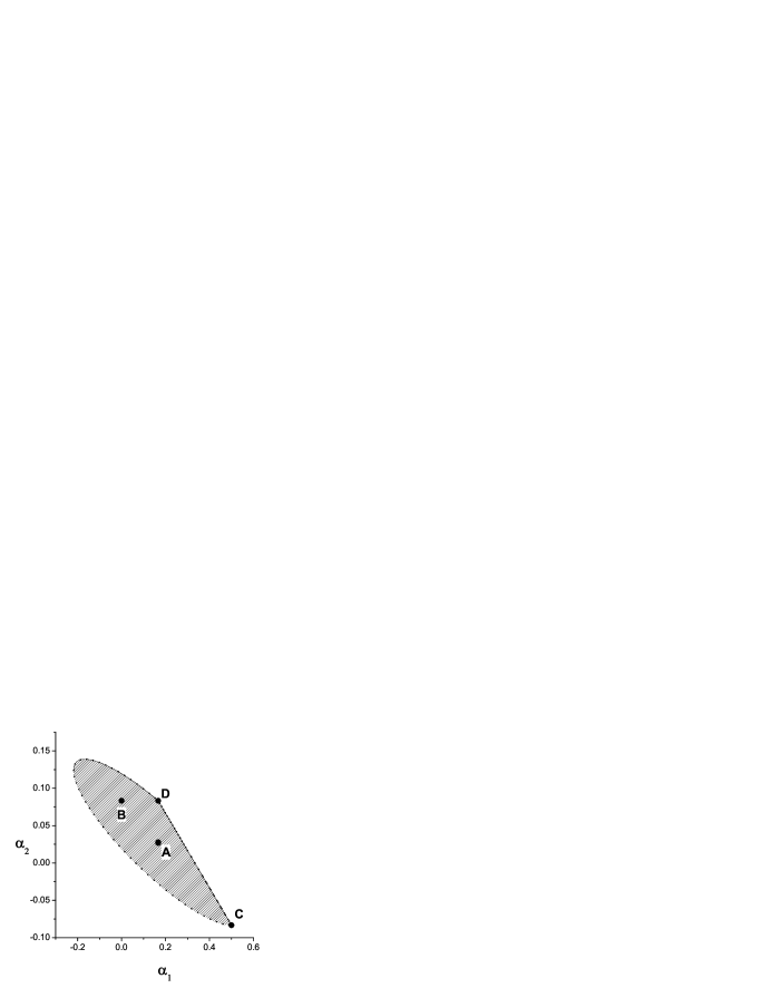
Figure 1: Eqs. $(\ref{hameqrxi1}),(\ref{hamxi0a})-(\ref{hamxi2a})$ with $g\neq 0$ are stable for any $(\alpha_{1},\,\alpha_{2})$ inside the filled area. Point $A$ corresponds to the centre of ellipse, $(\alpha_{1},\,\alpha_{2})=(\frac{1}{6},\,\frac{1}{36})$. Point $B$ corresponds to the most stable system $(\ref{AB3dimensionless})$, $(\alpha_{1},\,\alpha_{2})=(0,\,\frac{1}{12})$. Points $C$, $(\alpha_{1},\,\alpha_{2})=(\frac{1}{2},\,-\frac{1}{12})$, and $D$, $(\alpha_{1},\,\alpha_{2})=(\frac{1}{6},\,\frac{1}{12})$, correspond to intersections of the ellipse defined in $(\ref{beta2cond})$ with the line $3\alpha_{1}+6\alpha_{2}=1$. lushnikovzakharovfig1.eps

Thus $\tilde{\nu}_{\bf k}^{2}<0$ for any $\lambda$ and $\rho\geq 0$ provided inequalities $(\ref{beta1cond})$ and $(\ref{beta2cond})$ hold. It corresponds in $(\alpha_{1},\,\alpha_{2})$ plane to the inner part of the ellipse defined by $(\ref{beta2cond})$ and bounded by two parallel lines defined by $(\ref{beta1cond})$ (see the filled area in Figure 1). The center of the ellipse is located at $\alpha_{1}=\frac{1}{6},\quad\alpha_{2}=\frac{1}{36}$ (point $A$ in Figure 1). So the choice of $\alpha_{1}$ and $\alpha_{2}$ is not unique for $g\neq 0$ in the limit $\Theta\to 0$ and is determined by $(\ref{beta1cond}),(\ref{beta2cond})$.

For $g=0$ Eqs. $(\ref{AB3dimensionless})$ are reduced to

$$\tilde{\tilde{A}}_{\bf k}=1+\lambda+\big{[}\frac{3}{2}\alpha_{1}+\frac{1}{4}+3\alpha_{2}\big{]}\lambda^{2}+O(\lambda\Theta),$$

$$\tilde{\tilde{\nu}}_{\bf k}^{2}=\big{[}-\frac{1}{4}+\frac{3}{2}\alpha_{1}+6\alpha_{2}\big{]}^{2}\lambda^{2}-\big{[}\frac{1}{4}+3\alpha_{2}+O(\lambda^{-1}\Theta)\big{]}\tilde{\tilde{A}}_{\bf k}+O(\lambda\Theta),$$

$$\tilde{\tilde{\nu}}_{\bf k}^{2}=\frac{\xi_{0}^{2}}{\lambda^{2}(\hat{A}R_{0})^{2}}(\nu_{\bf k}+iG_{\bf k})^{2}.$$ (69)

It follows from Eq. $(\ref{AB3dimensionlessg0})$ that $\tilde{\tilde{\nu}}_{\bf k}^{2}<0$ in the limit $\Theta\to 0$ provided condition $(\ref{beta2cond})$ is satisfied, which corresponds in $(\alpha_{1},\,\alpha_{2})$ plane to the inner part of the ellipse defined by $(\ref{beta2cond})$ (see Figure 2) in contrast with the case of nonzero gravity.

For $k\to\infty$ we get from $(\ref{AB3})$ for $g\neq 0$:

$$\nu_{\bf k}=-i{\bf k}\cdot\nabla R_{0}\pm ik^{5/2}g^{1/2}3^{1/2}\big{[}\frac{3}{2}\alpha_{1}+\frac{1}{4}+3\alpha_{2}\big{]}^{1/2}$$

$$\times\big{[}\frac{1}{4}-\alpha_{2}-\frac{\alpha_{1}}{2}\big{]}^{1/2}\xi_{0}^{2}$$ (70)

and

$$\nu_{\bf k}=-i{\bf k}\cdot\nabla R_{0}\pm ik^{2}2^{-3/2}3$$

$$\times\big{[}-2\alpha_{1}^{2}+4\alpha_{2}(1-6\alpha_{2})+\alpha_{1}(1-12\alpha_{2})]^{1/2}\xi_{0}\hat{A}R_{0}$$ (71)

for $g=0$.

Note that for parameters satisfying inequalities $(\ref{beta1cond}),(\ref{beta2cond})$, the real part of $\nu_{\bf k}$ is zero even for $kh\sim 1$, where $\nu_{\bf k}$ takes the following form:

$$\nu_{\bf k}=-i{\bf k}\cdot\nabla R_{0}\pm iA_{k}^{1/2}\big{[}g+(\frac{1}{4}+3\alpha_{2})\,A_{k}(\hat{A}R_{0})^{2}\big{]}^{1/2},$$ (72)

so that in new canonical variables $(\ref{vdef}),(\ref{beta1cond}),(\ref{beta2cond})$ the instability is absent even for intermediate values of $k\sim 1/h.$ Another remark is that these variables leave problem well-posed for $\sigma\neq 0$ also but that case is not so interesting because Eqs. $(\ref{hameqrxi1}),(\ref{hamxi0a}),(\ref{hamxi1a}),(\ref{hamxi2a})$ well-posed even in original variables $\eta,\ \psi$ for $\sigma\neq 0$.

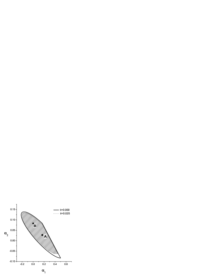
Figure 3: Shrinking of the stable region for small but nonzero $\Theta$ for $g\neq 0.$ Solid curve corresponds to $\Theta=0$. Area inside dotted curve corresponds to the stable region for $\Theta=0.025.$ Dotted curve is obtained numerically for Eq. $(\ref{AB3dimensionless})$ where we set as example $O(\lambda\Theta)=-\lambda\Theta,\ O(\lambda^{-1}\rho\Theta)=\lambda^{-1}\rho\Theta,\ O(\lambda\rho\Theta)=-\lambda\rho\Theta.$ Points $A,\,B$ are defined in Figure 1. lushnikovzakharovfig3.eps

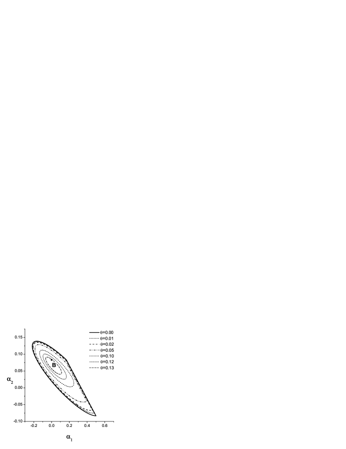
Figure 4: A series of curves corresponding to shrinking of the stable region as a function of $\Theta$ for $g\neq 0$. For $\Theta<0.1$, the width of region between solid curve ($\Theta=0$) and curves with $\Theta\neq 0$ scales approximately as $\Theta$. For $\Theta>0.1$, the stable region quickly shrinks to zero as $\Theta$ approaches $\simeq 0.1389$. Similar to Figure 3, all curves are calculated numerically with assumptions $O(\lambda\Theta)=-\lambda\Theta,\ O(\lambda^{-1}\rho\Theta)=\lambda^{-1}\rho\Theta,\ O(\lambda\rho\Theta)=-\lambda\rho\Theta.$ lushnikovzakharovfig4.eps

Now we make the second step and assume that $\Theta$ is small but nonzero in Eqs. $(\ref{AB3dimensionless})$ and $(\ref{AB3dimensionlessg0})$. Terms $O(\ldots\Theta)$ in Eqs. $(\ref{AB3dimensionless})$ and $(\ref{AB3dimensionlessg0})$ are not sign-definite and their values depends on horizontal coordinates $x,\,y$ and time according to dynamical Eqs. $(\ref{hameqrxi1}),(\ref{hamxi0a}),(\ref{hamxi1a}),(\ref{hamxi2a})$. Generally these terms result in shrinking of the area of stability, $\tilde{\nu}_{\bf k}^{2}<0$ in $(\alpha_{1},\,\alpha_{2})$ plane. Figures 3 and 4 show shrinking of the stability area for the particular choice of terms $O(\ldots\Theta)$ for $g\neq 0$. Each curve in Figure 4 corresponds to the stability boundary, $\max\limits_{\lambda,\,\rho}\tilde{\nu}_{\bf k}^{2}=0,$ for the particular value of $\Theta.$ The additional requirement is that

$$\frac{b_{1}}{12}\Theta(2+b_{1}\Theta)<\alpha_{2}+\frac{\alpha_{1}}{2}<\frac{1}{6}+\frac{b_{2}}{12}\Theta(2-b_{2}\Theta),$$ (73)

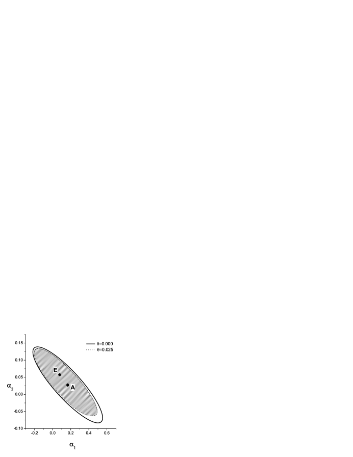
Figure 5: Shrinking of the stable region for small but nonzero $\Theta$ for $g=0.$ Solid curve corresponds to $\Theta=0$. Area inside dotted curve corresponds to the stable region for $\Theta=0.025.$ Dotted curve is obtained numerically for Eq. $(\ref{AB3dimensionless})$ where we set as example $O(\lambda\Theta)=-\lambda\Theta,\ O(\lambda^{-1}\Theta)=\lambda^{-1}\Theta.$ Points $A,\,E$ are defined in Figure 2. lushnikovzakharovfig5.eps

which is a generalization of $(\ref{beta1cond})$ for nonzero $\Theta$. Here we assume $O(\lambda\Theta)=b_{1}\lambda\Theta$ and $O(\lambda\Theta)=b_{2}\lambda\Theta$ in rhs of Eqs. $(\ref{AB3dimensionless})$ for $\tilde{\tilde{A}}_{\bf k}$ and $\tilde{\tilde{B}}_{\bf k}$, respectively. Calculating curves in Figures 3 and 4 we set $b_{1}=b_{2}=-1$ as a typical example. Condition $(\ref{beta1condTheta})$ result in additional cutting of curves $\max\limits_{\lambda,\,\rho}\tilde{\nu}_{\bf k}^{2}=0$ in Figures 3 and 4 for $\Theta=0,\,0.01,\,0.02,\,0.025$ and $0.05.$ The system $(\ref{AB3dimensionless})$ is stable inside each curve in Figure 4 for given $\Theta.$ For $\Theta<0.1$, the width of region between solid curve ($\Theta=0$) and curves with $\Theta\neq 0$ scales approximately as $\Theta$. For $\Theta>0.1$ the region of stability quickly shrinks to zero as $\Theta$ approaches $\simeq 0.1389$. Note that these numerical values are non-universal and depend on the numerical coefficient in $O(\ldots\Theta)$ terms. In a similar way, Figures 5,6 show shrinking of the stability area for zero gravity case.

Our objective is to find parameters $\alpha_{1},\,\alpha_{2}$ corresponding to stability, $\tilde{\nu}_{\bf k}^{2}<0$, with the largest possible $\Theta$. For the case $g\neq 0$ this is achieved if the maximum of $\tilde{\nu}_{\bf k}^{2}|_{\Theta=0}$, as a function of $\lambda,\,\rho$, is not only negative but minimum as a function of $\alpha_{1}$ and $\alpha_{2}$, i.e. we want to find $\min\limits_{\alpha_{1},\,\alpha_{2}}\max\limits_{\lambda,\,\rho}\tilde{\nu}_{\bf k}^{2}\big{|}_{\Theta=0}$. This ensures that the system $(\ref{AB3dimensionless})$ is the most stable system for $\Theta\to 0$ or, in other words, the system is the most rigid one. Because $\rho\geq 0$ we have to set $\rho=0$ to find $\max\limits_{\lambda,\,\rho}\tilde{\nu}_{\bf k}^{2}$. Then we obtain that $\min\limits_{\alpha_{1},\,\alpha_{2}}\max\limits_{\lambda,\,\rho}\tilde{\nu}_{\bf k}^{2}=\tilde{\nu}_{\bf k}^{2}\big{|}_{\rho=0,\,\lambda=0}=-1$. This minimum is attained provided $3\alpha_{1}+6\alpha_{2}=-1/2$ and $\frac{1}{6}(1-\sqrt{5})<\alpha_{1}<1/3$. We also want to have the most stable system for $k\to\infty$ ($\rho\to\infty$ and $\lambda\to\infty$). This is achieved provided the coefficients in front of the leading order terms $\lambda^{4}$ and $\lambda^{2}\rho$ in $\tilde{\nu}_{\bf k}^{2}$ are minimums. The coefficient for $\lambda^{4}$ is already minimum from condition $3\alpha_{1}+6\alpha_{2}=1/2$, while the coefficient for $\lambda^{2}\rho$ is $-3/16+9\alpha_{1}^{2}/4$, i.e. we have minimum for

$$\alpha_{1}=0,\quad\alpha_{2}=1/12,\quad g\neq 0,$$ (74)

which corresponds to point $B$ in Figure 1. This choice of parameters $\alpha_{1}$ and $\alpha_{2}$ is optimal to keep the system $(\ref{AB3dimensionless})$ stable for the largest possible $\Theta$, i.e. for the largest possible nonlinearity.

In a similar way, for zero gravity, $g=0,$ the system $(\ref{AB3dimensionlessg0})$ is the most stable provided we find $\alpha_{1},\,\alpha_{2}$ which correspond to $\min\limits_{\alpha_{1},\,\alpha_{2}}\max\limits_{\lambda}\tilde{\tilde{\nu}}_{\bf k}^{2}\big{|}_{\Theta=0}$ for Eqs. $(\ref{AB3dimensionlessg0})$. Maximum $\max\limits_{\lambda}\tilde{\tilde{\nu}}_{\bf k}^{2}\big{|}_{\Theta=0}$ is attained for

$$\lambda=\frac{(1+12\alpha_{2})}{9}\big{[}2\alpha_{1}^{2}+4\alpha_{2}(6\alpha_{2}-1)+\alpha_{1}(12\alpha_{2}-1)\big{]}^{-1},$$

and $\min\limits_{\alpha_{1},\,\alpha_{2}}\max\limits_{\lambda}\tilde{\tilde{\nu}}_{\bf k}^{2}\big{|}_{\Theta=0}=\frac{2}{3}(-2+\sqrt{3})$ is attained provided

$$\alpha_{1}=-\frac{1}{2}+3^{-1/2},\quad\alpha_{2}=\frac{1}{4}-3^{3/2},\quad g=0,$$ (75)

which corresponds to point $E$ in Figure 2. This choice of parameters $\alpha_{1}$ and $\alpha_{2}$ is optimal to keep the system $(\ref{AB3dimensionless})$ stable for the largest possible $\Theta$, i.e. for the largest possible nonlinearity.

Thus we can choose $\alpha_{1},\,\alpha_{2}$ from the conditions $(\ref{beta1cond})$ and $(\ref{beta2cond})$ to make Eqs. $(\ref{hameqrxi1}),(\ref{hamxi0a})-(\ref{hamxi2a})$ (or, equivalently, Eqs. $(\ref{dynamicsRxi1a}),(\ref{dynamicsRxi1b})$) well-posed for any value of $\sigma,\,g$ and arbitrary depth of fluid. To find dynamics of free surface, one can solve Eqs. for $R,\,\xi$ using Eqs. $(\ref{hameqrxi1}),(\ref{hamxi0a})-(\ref{hamxi2a})$ and conditions $(\ref{beta1cond}),(\ref{beta2cond}).$ This is the main result of this Article. To recover physical variables $\Psi,\,\eta$ from given $R,\,\xi$ one can use Eqs. $(\ref{etaeq1}),(\ref{psieq1}),(\ref{vdef}).$

Now we can return to the comment in Section 5 about interpretation of ill-posedness of Eqs. $(\ref{hamfoureq1}),(\ref{ham0})-(\ref{ham2})$ as violation of perturbation expansion $(\ref{hamserdef})$ for $k\eta_{0}\gtrsim 1.$ For the new canonical variables $\xi,\,R$ perturbation expansion is still formally violated for $k\xi_{0}\gtrsim 1$ because contribution from the quadratic Hamiltonian $(\ref{H2linxiR}),(\ref{AB3})$ is not small compare with other terms in the Hamiltonian $(\ref{hamxi0a})-(\ref{hamxi2a})$. However this violation does cause any problem because there is no short wavelength instability in the new canonical variables and the system $(\ref{hameqrxi1}),(\ref{hamxi0a})-(\ref{hamxi2a})$ is well-posed. In other words, the new canonical variables $\xi,\,R$ provide purely physical way to regularize short wavelengths without introduction any artificial viscosity.

As follows from Eqs. $(\ref{beta1cond}),(\ref{beta2cond}),$ the new canonical variables $\xi,\,R$ are not uniquely determined from the condition of well-posedness of the dynamical Eqs. $(\ref{hameqrxi1}),(\ref{hamxi0a})-(\ref{hamxi2a})$ because parameters $(\alpha_{1},\,\alpha_{2})$ can take any valued from filled area in Figures 1 and 2. However the choice of $(\alpha_{1},\,\alpha_{2})$ is unique provided we additionally require the system $(\ref{hameqrxi1}),(\ref{hamxi0a})-(\ref{hamxi2a})$ to be free of short wavelength instability for the largest possible slopes $\Theta$, i.e. for the largest possible nonlinearity. This gives the conditions $(\ref{alpha1alpha2p1p6})$ for $g\neq 0$ and $(\ref{alpha1alpha2p1p6g0})$ for $g=0.$ We refer to the variables $\xi,\,R$, defined in Eqs. $(\ref{etaeq1}),(\ref{psieq1}),(\ref{vdef}),(\ref{alpha1alpha2p1p6})$ and $(\ref{alpha1alpha2p1p6g0})$, as the optimal canonical variables. For some extent similar results were obtained by Dyachenko Dyachenko2004 for particular case of two-dimensional flow. We conjecture that the optimal canonical variables, which allow well-posedness of the dynamical Eqs., exist in all orders of nonlinearity. However additional research necessary to decide if the optimal canonical variables exist and unique in higher (fifth etc.) order of nonlinearity. We also conjecture that the optimal canonical variables $\xi,\,R$ would allow simulation with higher steepness compare with standard variables $\Psi,\,\eta.$

IX Special cases

There are a number of important special cases of the optimal canonical variables. Here we use $(\ref{alpha1alpha2p1p6})$ and $(\ref{alpha1alpha2p1p6g0})$. We give here expression for the Hamiltonian only. The dynamical Eqs. can be obtained either from $(\ref{hameqrxi1})$ or directly from Eqs. $(\ref{dynamicsRxi1a}),(\ref{dynamicsRxi1b})$.

IX.1 Deep water limit

For $g\neq 0,\ h\to\infty$, $A_{k}=k$ and Eqs. $(\ref{hamxi0a})-(\ref{hamxi2a})$ take the form

$$H_{0}=\frac{1}{2}\int\Big{\{}k|R_{\bf k}|^{2}+B_{k}|\xi_{\bf k}|^{2}\Big{\}}d{\bf k},\quad B_{k}=g+\sigma k^{2},$$ (76)

$$H_{1}=\frac{1}{4\pi}\int\Big{[}-({\bf k}_{1}\cdot{\bf k}_{2})R_{{\bf k}_{1}}R_{{\bf k}_{2}}-\frac{1}{6}(k_{1}B_{1}+k_{2}B_{2}+k_{3}B_{3})\xi_{{\bf k}_{1}}\xi_{{\bf k}_{2}}\Big{]}$$

$$\times\xi_{{\bf k}_{3}}\delta({\bf k}_{1}+{\bf k}_{2}+{\bf k}_{3})d{\bf k}_{1}d{\bf k}_{2}d{\bf k}_{3},$$ (77)

$$H_{2}=\frac{1}{8(2\pi)^{2}}\int\Big{\{}({\bf k}_{1}\cdot{\bf k}_{2})(|{\bf k}_{1}+{\bf k}_{2}|-k_{1}-k_{2})$$

$$-(k_{1}^{2}k_{2}+k_{2}^{2}k_{1})$$

$$+\frac{1}{2}k_{1}k_{2}\big{[}|{\bf k}_{1}+{\bf k}_{3}|+|{\bf k}_{2}+{\bf k}_{3}|+|{\bf k}_{1}+{\bf k}_{4}|+|{\bf k}_{2}+{\bf k}_{4}|\big{]}$$

$$+\frac{1}{4}k_{1}k_{2}\big{[}|{\bf k}_{1}+{\bf k}_{2}|+|{\bf k}_{3}+{\bf k}_{4}|\big{]}\Big{\}}$$

$$\times R_{{\bf k}_{1}}R_{{\bf k}_{2}}\xi_{{\bf k}_{3}}\xi_{{\bf k}_{4}}\delta({\bf k}_{1}+{\bf k}_{2}+{\bf k}_{3}+{\bf k}_{4})d{\bf k}_{1}d{\bf k}_{2}d{\bf k}_{3}d{\bf k}_{4}$$

$$+\frac{1}{8(2\pi)^{2}}\int\Big{\{}-\sigma({\bf k}_{1}\cdot{\bf k}_{2})({\bf k}_{3}\cdot{\bf k}_{4})+\frac{1}{4}|{\bf k}_{1}+{\bf k}_{2}|^{2}B_{1+2}+k_{3}B_{3}|{\bf k}_{1}+{\bf k}_{2}|$$

$$-\frac{1}{6}B_{1}k_{1}(|{\bf k}_{2}+{\bf k}_{3}|+|{\bf k}_{2}+{\bf k}_{4}|+|{\bf k}_{3}+{\bf k}_{4}|)\Big{\}}$$

$$\times\xi_{{\bf k}_{1}}\xi_{{\bf k}_{2}}\xi_{{\bf k}_{3}}\xi_{{\bf k}_{4}}\delta({\bf k}_{1}+{\bf k}_{2}+{\bf k}_{3}+{\bf k}_{4})d{\bf k}_{1}d{\bf k}_{2}d{\bf k}_{3}d{\bf k}_{4}.$$ (78)

IX.1.1 Zero gravity and capillarity $g=\sigma=0$

$$H_{0}=\frac{1}{2}\int k|R_{\bf k}|^{2}d{\bf k},$$ (79)

$$H_{1}=-\frac{1}{4\pi}\int({\bf k}_{1}\cdot{\bf k}_{2})R_{{\bf k}_{1}}R_{{\bf k}_{2}}\xi_{{\bf k}_{3}}\delta({\bf k}_{1}+{\bf k}_{2}+{\bf k}_{3})d{\bf k}_{1}d{\bf k}_{2}d{\bf k}_{3},$$ (80)

$$H_{2}=\frac{1}{8(2\pi)^{2}}\int\Big{\{}({\bf k}_{1}\cdot{\bf k}_{2})(|{\bf k}_{1}+{\bf k}_{2}|-k_{1}-k_{2})$$

$$+(-\frac{5}{2}+\sqrt{3})(k_{1}^{2}k_{2}+k_{2}^{2}k_{1})$$

$$+(1-3^{5/2})k_{1}k_{2}\big{[}|{\bf k}_{1}+{\bf k}_{3}|+|{\bf k}_{2}+{\bf k}_{3}|+|{\bf k}_{1}+{\bf k}_{4}|+|{\bf k}_{2}+{\bf k}_{4}|\big{]}$$

$$+(\frac{3}{4}-3^{5/2})k_{1}k_{2}\big{[}|{\bf k}_{1}+{\bf k}_{2}|+|{\bf k}_{3}+{\bf k}_{4}|\big{]}\Big{\}}$$

$$\times R_{{\bf k}_{1}}R_{{\bf k}_{2}}\xi_{{\bf k}_{3}}\xi_{{\bf k}_{4}}\delta({\bf k}_{1}+{\bf k}_{2}+{\bf k}_{3}+{\bf k}_{4})d{\bf k}_{1}d{\bf k}_{2}d{\bf k}_{3}d{\bf k}_{4}.$$ (81)

IX.1.2 Zero gravity, $g=0,$ and nonzero capillarity $\sigma\neq 0$

$$H_{0}=\frac{1}{2}\int\Big{\{}k|R_{\bf k}|^{2}+\sigma k^{2}|\xi_{\bf k}|^{2}\Big{\}}d{\bf k},$$ (82)

$$H_{1}=\frac{1}{4\pi}\int\Big{[}-({\bf k}_{1}\cdot{\bf k}_{2})R_{{\bf k}_{1}}R_{{\bf k}_{2}}-\frac{\sigma}{6}(k_{1}^{3}+k_{2}^{3}+k_{3}^{3})\xi_{{\bf k}_{1}}\xi_{{\bf k}_{2}}\Big{]}$$

$$\times\xi_{{\bf k}_{3}}\delta({\bf k}_{1}+{\bf k}_{2}+{\bf k}_{3})d{\bf k}_{1}d{\bf k}_{2}d{\bf k}_{3},$$ (83)

$$H_{2}=\frac{1}{8(2\pi)^{2}}\int\Big{\{}({\bf k}_{1}\cdot{\bf k}_{2})(|{\bf k}_{1}+{\bf k}_{2}|-k_{1}-k_{2})$$

$$+(-\frac{5}{2}+\sqrt{3})(k_{1}^{2}k_{2}+k_{2}^{2}k_{1})$$

$$+(1-3^{5/2})k_{1}k_{2}\big{[}|{\bf k}_{1}+{\bf k}_{3}|+|{\bf k}_{2}+{\bf k}_{3}|+|{\bf k}_{1}+{\bf k}_{4}|+|{\bf k}_{2}+{\bf k}_{4}|\big{]}$$

$$+(\frac{3}{4}-3^{5/2})k_{1}k_{2}\big{[}|{\bf k}_{1}+{\bf k}_{2}|+|{\bf k}_{3}+{\bf k}_{4}|\big{]}\Big{\}}$$

$$\times R_{{\bf k}_{1}}R_{{\bf k}_{2}}\xi_{{\bf k}_{3}}\xi_{{\bf k}_{4}}\delta({\bf k}_{1}+{\bf k}_{2}+{\bf k}_{3}+{\bf k}_{4})d{\bf k}_{1}d{\bf k}_{2}d{\bf k}_{3}d{\bf k}_{4}$$

$$+\frac{\sigma}{8(2\pi)^{2}}\int\Big{\{}-({\bf k}_{1}\cdot{\bf k}_{2})({\bf k}_{3}\cdot{\bf k}_{4})+\frac{1}{4}|{\bf k}_{1}+{\bf k}_{2}|^{4}+k_{3}^{3}|{\bf k}_{1}+{\bf k}_{2}|$$

$$-k_{1}^{3}\big{[}(-1+3^{-1/2})k_{1}+(\frac{1}{2}-3^{3/2}2)(|{\bf k}_{2}+{\bf k}_{3}|+|{\bf k}_{2}+{\bf k}_{4}|+|{\bf k}_{3}+{\bf k}_{4}|)\big{]}\Big{\}}$$

$$\times\xi_{{\bf k}_{1}}\xi_{{\bf k}_{2}}\xi_{{\bf k}_{3}}\xi_{{\bf k}_{4}}\delta({\bf k}_{1}+{\bf k}_{2}+{\bf k}_{3}+{\bf k}_{4})d{\bf k}_{1}d{\bf k}_{2}d{\bf k}_{3}d{\bf k}_{4}.$$ (84)

IX.1.3 Nonzero gravity, $g\neq 0,$ and zero capillarity $\sigma=0$

$$H_{0}=\frac{1}{2}\int\Big{\{}k|R_{\bf k}|^{2}+g|\xi_{\bf k}|^{2}\Big{\}}d{\bf k},$$ (85)

$$H_{1}=\frac{1}{4\pi}\int\Big{[}-({\bf k}_{1}\cdot{\bf k}_{2})R_{{\bf k}_{1}}R_{{\bf k}_{2}}-\frac{g}{6}(k_{1}+k_{2}+k_{3})\xi_{{\bf k}_{1}}\xi_{{\bf k}_{2}}\Big{]}$$

$$\times\xi_{{\bf k}_{3}}\delta({\bf k}_{1}+{\bf k}_{2}+{\bf k}_{3})d{\bf k}_{1}d{\bf k}_{2}d{\bf k}_{3},$$ (86)

$$H_{2}=\frac{1}{8(2\pi)^{2}}\int\Big{\{}({\bf k}_{1}\cdot{\bf k}_{2})(|{\bf k}_{1}+{\bf k}_{2}|-k_{1}-k_{2})-(k_{1}^{2}k_{2}+k_{2}^{2}k_{1})$$

$$+\frac{1}{2}k_{1}k_{2}\big{[}|{\bf k}_{1}+{\bf k}_{3}|+|{\bf k}_{2}+{\bf k}_{3}|+|{\bf k}_{1}+{\bf k}_{4}|+|{\bf k}_{2}+{\bf k}_{4}|\big{]}$$

$$+\frac{1}{4}k_{1}k_{2}\big{[}|{\bf k}_{1}+{\bf k}_{2}|+|{\bf k}_{3}+{\bf k}_{4}|\big{]}\Big{\}}$$

$$\times R_{{\bf k}_{1}}R_{{\bf k}_{2}}\xi_{{\bf k}_{3}}\xi_{{\bf k}_{4}}\delta({\bf k}_{1}+{\bf k}_{2}+{\bf k}_{3}+{\bf k}_{4})d{\bf k}_{1}d{\bf k}_{2}d{\bf k}_{3}d{\bf k}_{4}$$

$$+\frac{g}{8(2\pi)^{2}}\int\Big{\{}\frac{1}{4}|{\bf k}_{1}+{\bf k}_{2}|^{2}+k_{3}|{\bf k}_{1}+{\bf k}_{2}|$$

$$-\frac{1}{6}k_{1}(|{\bf k}_{2}+{\bf k}_{3}|+|{\bf k}_{2}+{\bf k}_{4}|+|{\bf k}_{3}+{\bf k}_{4}|)\Big{\}}$$

$$\times\xi_{{\bf k}_{1}}\xi_{{\bf k}_{2}}\xi_{{\bf k}_{3}}\xi_{{\bf k}_{4}}\delta({\bf k}_{1}+{\bf k}_{2}+{\bf k}_{3}+{\bf k}_{4})d{\bf k}_{1}d{\bf k}_{2}d{\bf k}_{3}d{\bf k}_{4}.$$ (87)

IX.2 Shallow water limit

Shallow water limit corresponds to $kh\to 0$. In that limit $A_{k}\to k^{2}h$. Eqs. $(\ref{hamxi0a})-(\ref{hamxi2a})$ take the following form for $g\neq 0:$

$$H_{0}=\frac{1}{2}\int\Big{\{}k^{2}h|R_{\bf k}|^{2}+B_{k}|\xi_{\bf k}|^{2}\Big{\}}d{\bf k},\quad B_{k}=g+\sigma k^{2},$$ (88)

$$H_{1}=\frac{1}{4\pi}\int\Big{[}-({\bf k}_{1}\cdot{\bf k}_{2})R_{{\bf k}_{1}}R_{{\bf k}_{2}}-\frac{h}{6}(k_{1}^{2}B_{1}+k_{2}^{2}B_{2}+k_{3}^{2}B_{3})\xi_{{\bf k}_{1}}\xi_{{\bf k}_{2}}\Big{]}$$

$$\times\xi_{{\bf k}_{3}}\delta({\bf k}_{1}+{\bf k}_{2}+{\bf k}_{3})d{\bf k}_{1}d{\bf k}_{2}d{\bf k}_{3},$$ (89)

$$H_{2}=\frac{h}{8(2\pi)^{2}}\int\Big{\{}2({\bf k}_{1}\cdot{\bf k}_{2})^{2}-(k_{1}^{2}k_{2}^{2}+k_{2}^{2}k_{1}^{2})$$

$$+h^{2}\frac{1}{2}k_{1}^{2}k_{2}^{2}\big{[}|{\bf k}_{1}+{\bf k}_{3}|^{2}+|{\bf k}_{2}+{\bf k}_{3}|^{2}+|{\bf k}_{1}+{\bf k}_{4}|^{2}+|{\bf k}_{2}+{\bf k}_{4}|^{2}\big{]}$$

$$+h^{2}\frac{1}{4}k_{1}^{2}k_{2}^{2}\big{[}|{\bf k}_{1}+{\bf k}_{2}|^{2}+|{\bf k}_{3}+{\bf k}_{4}|^{2}\big{]}\Big{\}}$$

$$\times R_{{\bf k}_{1}}R_{{\bf k}_{2}}\xi_{{\bf k}_{3}}\xi_{{\bf k}_{4}}\delta({\bf k}_{1}+{\bf k}_{2}+{\bf k}_{3}+{\bf k}_{4})d{\bf k}_{1}d{\bf k}_{2}d{\bf k}_{3}d{\bf k}_{4}$$

$$+\frac{1}{8(2\pi)^{2}}\int\Big{\{}-\sigma({\bf k}_{1}\cdot{\bf k}_{2})({\bf k}_{3}\cdot{\bf k}_{4})$$

$$+\frac{h^{2}}{4}|{\bf k}_{1}+{\bf k}_{2}|^{4}B_{1+2}+h^{2}k_{3}^{2}B_{3}|{\bf k}_{1}+{\bf k}_{2}|^{2}$$

$$-\frac{B_{1}k_{1}^{2}h^{2}}{6}(|{\bf k}_{2}+{\bf k}_{3}|^{2}+|{\bf k}_{2}+{\bf k}_{4}|^{2}+|{\bf k}_{3}+{\bf k}_{4}|^{2})\Big{\}}$$

$$\times\xi_{{\bf k}_{1}}\xi_{{\bf k}_{2}}\xi_{{\bf k}_{3}}\xi_{{\bf k}_{4}}\delta({\bf k}_{1}+{\bf k}_{2}+{\bf k}_{3}+{\bf k}_{4})d{\bf k}_{1}d{\bf k}_{2}d{\bf k}_{3}d{\bf k}_{4}.$$ (90)

IX.2.1 Zero gravity and capillarity $g=\sigma=0$

$$H_{0}=\frac{1}{2}\int k^{2}h|R_{\bf k}|^{2}d{\bf k},$$ (91)

$$H_{1}=-\frac{1}{4\pi}\int({\bf k}_{1}\cdot{\bf k}_{2})R_{{\bf k}_{1}}R_{{\bf k}_{2}}\xi_{{\bf k}_{3}}\delta({\bf k}_{1}+{\bf k}_{2}+{\bf k}_{3})d{\bf k}_{1}d{\bf k}_{2}d{\bf k}_{3},$$ (92)

$$H_{2}=\frac{h}{8(2\pi)^{2}}\int\Big{\{}2({\bf k}_{1}\cdot{\bf k}_{2})^{2}+(-\frac{5}{2}+\sqrt{3})(k_{1}^{2}k_{2}^{2}+k_{2}^{2}k_{1}^{2})$$

$$+h^{2}(1-3^{5/2})k_{1}^{2}k_{2}^{2}\big{[}|{\bf k}_{1}+{\bf k}_{3}|^{2}+|{\bf k}_{2}+{\bf k}_{3}|^{2}+|{\bf k}_{1}+{\bf k}_{4}|^{2}+|{\bf k}_{2}+{\bf k}_{4}|^{2}\big{]}$$

$$+h^{2}(\frac{3}{4}-3^{5/2})k_{1}^{2}k_{2}^{2}\big{[}|{\bf k}_{1}+{\bf k}_{2}|^{2}+|{\bf k}_{3}+{\bf k}_{4}|^{2}\big{]}\Big{\}}$$

$$\times R_{{\bf k}_{1}}R_{{\bf k}_{2}}\xi_{{\bf k}_{3}}\xi_{{\bf k}_{4}}\delta({\bf k}_{1}+{\bf k}_{2}+{\bf k}_{3}+{\bf k}_{4})d{\bf k}_{1}d{\bf k}_{2}d{\bf k}_{3}d{\bf k}_{4}.$$ (93)

IX.2.2 Zero gravity, $g=0,$ and nonzero capillarity $\sigma\neq 0$

$$H_{0}=\frac{1}{2}\int\Big{\{}k^{2}h|R_{\bf k}|^{2}+\sigma k^{2}|\xi_{\bf k}|^{2}\Big{\}}d{\bf k},$$ (94)

$$H_{1}=\frac{1}{4\pi}\int\Big{[}-({\bf k}_{1}\cdot{\bf k}_{2})R_{{\bf k}_{1}}R_{{\bf k}_{2}}-\frac{\sigma h}{6}(k_{1}^{4}+k_{2}^{4}+k_{3}^{4})\xi_{{\bf k}_{1}}\xi_{{\bf k}_{2}}\Big{]}$$

$$\times\xi_{{\bf k}_{3}}\delta({\bf k}_{1}+{\bf k}_{2}+{\bf k}_{3})d{\bf k}_{1}d{\bf k}_{2}d{\bf k}_{3},$$ (95)

$$H_{2}=\frac{h}{8(2\pi)^{2}}\int\Big{\{}2({\bf k}_{1}\cdot{\bf k}_{2})^{2}+(-\frac{5}{2}+\sqrt{3})(k_{1}^{2}k_{2}^{2}+k_{2}^{2}k_{1}^{2})$$

$$+h^{2}(1-3^{5/2})k_{1}^{2}k_{2}^{2}\big{[}|{\bf k}_{1}+{\bf k}_{3}|^{2}+|{\bf k}_{2}+{\bf k}_{3}|^{2}+|{\bf k}_{1}+{\bf k}_{4}|^{2}+|{\bf k}_{2}+{\bf k}_{4}|^{2}\big{]}$$

$$+h^{2}(\frac{3}{4}-3^{5/2})k_{1}^{2}k_{2}^{2}\big{[}|{\bf k}_{1}+{\bf k}_{2}|^{2}+|{\bf k}_{3}+{\bf k}_{4}|^{2}\big{]}\Big{\}}$$

$$\times R_{{\bf k}_{1}}R_{{\bf k}_{2}}\xi_{{\bf k}_{3}}\xi_{{\bf k}_{4}}\delta({\bf k}_{1}+{\bf k}_{2}+{\bf k}_{3}+{\bf k}_{4})d{\bf k}_{1}d{\bf k}_{2}d{\bf k}_{3}d{\bf k}_{4}$$

$$+\frac{\sigma}{8(2\pi)^{2}}\int\Big{\{}-({\bf k}_{1}\cdot{\bf k}_{2})({\bf k}_{3}\cdot{\bf k}_{4})+\frac{h^{2}}{4}|{\bf k}_{1}+{\bf k}_{2}|^{6}+h^{2}k_{3}^{4}|{\bf k}_{1}+{\bf k}_{2}|^{2}$$

$$-k_{1}^{4}\big{[}(-1+3^{-1/2})+(\frac{1}{2}-3^{3/2}2)h^{2}(|{\bf k}_{2}+{\bf k}_{3}|^{2}+|{\bf k}_{2}+{\bf k}_{4}|^{2}+|{\bf k}_{3}+{\bf k}_{4}|^{2})\big{]}$$

$$\times\xi_{{\bf k}_{1}}\xi_{{\bf k}_{2}}\xi_{{\bf k}_{3}}\xi_{{\bf k}_{4}}\delta({\bf k}_{1}+{\bf k}_{2}+{\bf k}_{3}+{\bf k}_{4})d{\bf k}_{1}d{\bf k}_{2}d{\bf k}_{3}d{\bf k}_{4}.$$ (96)

IX.2.3 Nonzero gravity, $g\neq 0,$ and zero capillarity $\sigma=0$

$$H_{0}=\frac{1}{2}\int\Big{\{}k^{2}h|R_{\bf k}|^{2}+g|\xi_{\bf k}|^{2}\Big{\}}d{\bf k},$$ (97)

$$H_{1}=\frac{1}{4\pi}\int\Big{[}-({\bf k}_{1}\cdot{\bf k}_{2})R_{{\bf k}_{1}}R_{{\bf k}_{2}}-\frac{gh}{6}(k_{1}^{2}+k_{2}^{2}+k_{3}^{2})\xi_{{\bf k}_{1}}\xi_{{\bf k}_{2}}\Big{]}$$

$$\times\xi_{{\bf k}_{3}}\delta({\bf k}_{1}+{\bf k}_{2}+{\bf k}_{3})d{\bf k}_{1}d{\bf k}_{2}d{\bf k}_{3},$$ (98)

$$H_{2}=\frac{h}{8(2\pi)^{2}}\int\Big{\{}2({\bf k}_{1}\cdot{\bf k}_{2})^{2}-(k_{1}^{2}k_{2}^{2}+k_{2}^{2}k_{1}^{2})$$

$$+h^{2}\frac{1}{2}k_{1}^{2}k_{2}^{2}\big{[}|{\bf k}_{1}+{\bf k}_{3}|^{2}+|{\bf k}_{2}+{\bf k}_{3}|^{2}+|{\bf k}_{1}+{\bf k}_{4}|^{2}+|{\bf k}_{2}+{\bf k}_{4}|^{2}\big{]}$$

$$+h^{2}\frac{1}{4}k_{1}^{2}k_{2}^{2}\big{[}|{\bf k}_{1}+{\bf k}_{2}|^{2}+|{\bf k}_{3}+{\bf k}_{4}|^{2}\big{]}\Big{\}}$$

$$\times R_{{\bf k}_{1}}R_{{\bf k}_{2}}\xi_{{\bf k}_{3}}\xi_{{\bf k}_{4}}\delta({\bf k}_{1}+{\bf k}_{2}+{\bf k}_{3}+{\bf k}_{4})d{\bf k}_{1}d{\bf k}_{2}d{\bf k}_{3}d{\bf k}_{4}$$

$$+\frac{g}{8(2\pi)^{2}}\int\Big{\{}\frac{h^{2}}{4}|{\bf k}_{1}+{\bf k}_{2}|^{4}+h^{2}k_{3}^{2}|{\bf k}_{1}+{\bf k}_{2}|^{2}$$

$$-\frac{k_{1}^{2}h^{2}}{6}(|{\bf k}_{2}+{\bf k}_{3}|^{2}+|{\bf k}_{2}+{\bf k}_{4}|^{2}+|{\bf k}_{3}+{\bf k}_{4}|^{2})$$

$$\times\xi_{{\bf k}_{1}}\xi_{{\bf k}_{2}}\xi_{{\bf k}_{3}}\xi_{{\bf k}_{4}}\delta({\bf k}_{1}+{\bf k}_{2}+{\bf k}_{3}+{\bf k}_{4})d{\bf k}_{1}d{\bf k}_{2}d{\bf k}_{3}d{\bf k}_{4}.$$ (99)

X Conclusion

In conclusion, we found the optimal canonical variables for which the water wave problem is well-posed in the approximation which keeps terms up to fourth order in the Hamiltonian. The important question remain open if it is possible to make water wave equations well-posed by proper choice of canonical transform for higher-order corrections (fifth and higher order). We conjecture that such optimal canonical variables exist in all orders of nonlinearity.

Support was provided by US Army Corps of Engineers, RDT&E Programm, grant DACA # 42-00-C0044 (V.Z.), and to NSF grant # NDMS0072803 (V.Z.).

Figure 2: Eqs. $(\ref{hameqrxi1}),(\ref{hamxi0a})-(\ref{hamxi2a})$ with $g=0$ are stable for any $(\alpha_{1},\,\alpha_{2})$ inside the filled area. The filled area is bounded by the ellipse defined in $(\ref{beta2cond})$. Point $A$ corresponds to the centre of ellipse, $(\alpha_{1},\,\alpha_{2})=(\frac{1}{6},\,\frac{1}{36})$. Point $E$, $(\alpha_{1},\,\alpha_{2})=(-\frac{1}{2}+3^{-1/2},\,\frac{1}{4}-3^{3/2})$, corresponds to the most stable system $(\ref{AB3dimensionlessg0})$. lushnikovzakharovfig2.eps

Figure 6: A series of curves corresponding to shrinking of the stable region as a function of $\Theta$ for $g=0$. For $\Theta<0.1$, the width of region between solid curve ($\Theta=0$) and curves with $\Theta\neq 0$ scales approximately as $\Theta$. For $\Theta>0.1$, the stable region quickly shrinks to zero as $\Theta$ approaches $\simeq 0.1389$. Similar to Figure 5, all curves are calculated numerically with assumptions $O(\lambda\Theta)=-\lambda\Theta,\ O(\lambda^{-1}\Theta)=\lambda^{-1}\Theta.$ lushnikovzakharovfig6.eps