On Some Classes of mKdV Periodic Solutions

Abstract

We obtain exact periodic solutions of the positive and negative modified Kortweg-de Vries (mKdV) equations. We examine the dynamical stability of these solitary wave lattices through direct numerical simulations. While the positive mKdV breather lattice solutions are found to be unstable, the two-soliton lattice solution of the same equation is found to be stable. Similarly, a negative mKdV lattice solution is found to be stable. We also touch upon the implications of these results for the KdV equation.

1 Introduction

Among the soliton bearing nonlinear integrable equations, sine-Gordon, nonlinear Schrödinger (NLS), Korteweg-de Vries (KdV) and the modified Korteweg-de Vries (mKdV) are of special interest [2, 3, 4, 5, 6]. These equations possess exact breather solutions. Therefore, they may also have exact solutions in the form of a spatially periodic array of single breathers, i.e. breather lattices. Similarly to the sine-Gordon, NLS and KdV, the mKdV equation is also important in many physical contexts. For example, it appears in the context of ion acoustic solitons [7], van Alfvén waves in collisionless plasma [8], Schottky barrier transmission lines [9], models of traffic congestion [10] as well as phonons in anharmonic lattices [11]. Furthermore, the modelling of a subclass of hyperbolic surfaces [12], slag-metallic bath interfaces [13] as well as meandering ocean jets [14] is also related to the mKdV equation. The dynamics of thin elastic rods has also been demonstrated to be reducible to the mKdV equation [15]. Finally, if one studies the examples of surface dynamics that are purely local, yet maintain global constraints like conservation of perimeter and enclosed area, one finds that these dynamics are closely related to the KdV and mKdV hierarchies [16].

The nonlinear term in the mKdV equation ($6u^{2}u_{x}$) may assume either a positive or a negative sign. We will classify the equation as “positive mKdV” and “negative mKdV” if the prefactor is $+1$ or $-1$, respectively. In an earlier study, the stability of the sine-Gordon breather lattice was examined [17]. Recently, a particular form of an exact breather lattice solution was obtained in [18] for the positive mKdV equation and its stability was discussed.

The aim of the present Letter is to present a new class of periodic solutions both for the positive and for the negative mKdV equations. We also intend to examine the dynamical stability of these novel classes of solutions and particularly to illustrate that many of them can be dynamically stable. This is notably different from the behavior observed previously for breather lattice solutions in the models of [17, 18]. Furthermore, it is worth noting that the solutions of the negative mKdV are related to those of the KdV equation via the Miura transform [19]. Thus, our solutions can be translated into exact periodic solutions of the KdV equation as well. The latter is also a ubiquitous equation in a variety of fields ranging from conformal field theory to plasma physics.

Our presentation is structured as follows. In Sec. 2 we examine the breather lattice and two-soliton lattice solutions of the mKdV equation with positive sign of nonlinearity and discuss their stability. In Sec. 3 we examine periodic solutions of the mKdV equation with the negative sign of the nonlinearity. In Sec. 4 we briefly comment on the corresponding KdV solutions and follow that with our conclusions in Sec. 5.

2 Breather and Soliton Lattices of the Positive mKdV Equation

For a field $u(x,t)$, the positive mKdV equation is given by

$$u_{t}+6u^{2}u_{x}+u_{xxx}=0.$$ (1)

Using the ansatz

$$u=-2\frac{d}{dx}[\tan^{-1}\phi],$$ (2)

we are able to obtain several exact spatially periodic solutions. The first one is a breather lattice solution [18]

$$\phi=\alpha\rm sn(ax+bt+a_{0},k)\rm dn(cx+dt+c_{0},m),$$ (3)

where $a_{0},c_{0}$ are arbitrary constants. In fact, all the solutions discussed in this paper admit such constants even though we will not always display them hereafter. In this solution:

$$\alpha=-\frac{c}{a},~{}\frac{c^{4}}{a^{4}}=\frac{k}{(1-m)},~{}\frac{b}{a}=[a^{2}(1+k)-3c^{2}(2-m)],$$

$$\frac{d}{c}=[3a^{2}(1+k)-c^{2}(2-m)]\,,$$ (4)

while sn$(x,k)$, ($\rm cn(x,k)$ below), and $\rm dn(x,m)$ are Jacobi elliptic functions with modulus $k$ and $m$, respectively. This solution was studied in detail previously in [18]. For completeness, we discuss briefly the relevant results. In order to ensure periodicity of the solution (in space), a commensurability condition was postulated in that work. In its strict form (strong commensurability), this condition demands that the two elliptic function terms of Eq. (3) have the same period, i.e. $4K(k)/a=2K(m)/c$ (where $K(k)$ denotes the complete elliptic integral of the first kind). In its weaker form (weak commensurability), the condition demands that the periodicities are rational multiples of each other i.e.,

$$4p\frac{K(k)}{a}=2q\frac{K(m)}{c}$$ (5)

with $p,q\in Z_{+}^{\star}$, note that $p=q=1$ yields the strong commensurability as a special case. Both strong and weak forms, however, resulted in unstable dynamical evolutions of the breather lattice [18] (induced by means of numerical perturbations to the exact solution). We further showed that this solution could be stabilized through ac driving and damping. In the limit $k\rightarrow 0,m\rightarrow 1,$ but with ${k}/(1-m)=v^{4}$, this solution goes over to the well known single breather (bion) solution

$$\phi=-v\sin(ax+bt+a_{0})\rm sech(cx+dt+c_{0}).$$ (6)

Remarkably, it turns out that there is a different breather lattice solution to the positive mKdV equation given by

$$\phi=\alpha\rm cn(ax+bt+a_{1},k)\rm cn(cx+dt+c_{1},m),$$ (7)

where

$$\alpha^{2}=\frac{mk}{(1-m)(1-k)},~{}\frac{c^{4}}{a^{4}}=\frac{k(1-k)}{m(1-m)},$$

$$\frac{b}{a}=[a^{2}(1-2k)+3c^{2}(1-2m)],~{}\frac{d}{c}=[3a^{2}(1-2k)+c^{2}(1-2m)].$$ (8)

Notice that in the limit $k\rightarrow 0,m\rightarrow 1,a_{1}=\pi/2+a_{0}$ $c_{1}=c_{0}$ but with ${k}/(1-m)=v^{4}$, this solution also goes over to the same breather (bion) solution (6). However, for other values of $k,m$, the two breather lattice solutions (3) and (7) are quite different (see also the comparison of the right panel of Fig. 1). We should note here that the characterization of the solutions that we present as breather or two-soliton lattices is given on the basis of what their limiting (see e.g., Eq. (6)) profile looks like, as the elliptic functions asymptote to trigonometric/hyperbolic ones.

The dynamical stability of the breather lattice solution (7) was examined for both strong and weak commensurability by means of direct numerical simulations. The numerical scheme used here, motivated by the KdV discretization of Ref. [20] was analyzed previously in [18]. However, the results were also verified with different discretizations of the integrable model such as the ones proposed in [21]. In Fig. 1, we demonstrate a typical example of the dynamical evolution of the solution of Eqs. (7)-(8). We observe that similarly to the previously obtained breather lattice solution of [18], the breather lattice identified above is dynamically unstable in the mKdV equation and results in a few more strongly and many weakly localized peaks. Hence, the instability of mKdV breather lattices appears to be generic.

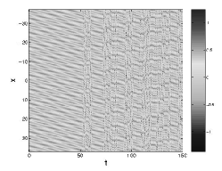
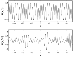
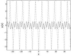
Figure 1: The left panel shows the x-t (i.e., space-time) evolution of the contour of the unstable breather lattice solution of the form of Eqs. (7)-(8); $a=1$, $k=0.5$, $c=1.707$ and $m=0.03$ (such that $K(k)/a=2K(m)/c$) were used in the initial conditions. The middle panel shows the spatial profile at $t=0$ (initial condition) and at $t=55$ (after the instability has set in). Finally, the right panel shows with a solid line the initial condition and with a dashed line the (other breather lattice) solution of Eqs. (3)-(4) for the same parameters.

Using the ansatz in terms of Eq. (2), we can obtain yet another novel family of solutions, namely a two-soliton lattice

$$\phi=\alpha\rm sc(ax+bt,k)\rm dn(cx+dt,m),$$ (9)

where $\alpha=-c/a$, $\rm sc(x,m)\equiv\rm sn(x,m)/\rm cn(x,m)$ and

$$\frac{c^{4}}{a^{4}}=\frac{1-k}{1-m},~{}~{}\frac{b}{a}=-[a^{2}(2-k)+3c^{2}(2-m)],$$

$$\frac{d}{c}=-[c^{2}(2-m)+3a^{2}(2-k)].$$ (10)

This solution can also be obtained from the breather lattice solution (3) by taking $a\rightarrow ia,b\rightarrow ib,\alpha\rightarrow-i\alpha$ and using the well known relations

$$\rm sn(ix,m)=i\frac{\rm sn(x,1-m)}{\rm cn(x,1-m)}\,,~{}~{}\rm dn(ix,m)=\frac{\rm dn(x,1-m)}{\rm cn(x,1-m)}\,,$$

$$\rm cn(ix,m)=\frac{1}{\rm cn(x,1-m)}\,.$$ (11)

In the limit $k\rightarrow 1,\,m\rightarrow 1$ but with $(1-k)/(1-m)=v^{4}$ this solution goes over to

$$\phi=-v\sinh[a(x-[1+3v^{2}]t)]\rm sech[av(x-[3+v^{2}]t)]~{},$$ (12)

which, except for $v=1$, is the well-known 2-soliton solution (hence the classification of this solution as a 2-soliton lattice). For $v=1$, however, it corresponds to the one-soliton solution. The latter implies $k=m$ and $c=a$ from Eq. (10).

An example of the dynamical evolution for the two-soliton lattice solution is shown in Fig. 2. As it can be seen, this solution persists unchanged for long dynamical evolutions (i.e., for times of the order of 150 in the arbitrary time units of the time evolution of Fig. 2), hence our numerical simulations indicate that it is dynamically stable.

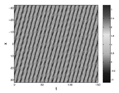
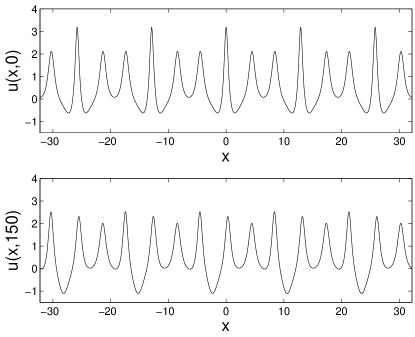
Figure 2: The left panel shows the spatio-temporal evolution of the contour plot of a two-soliton lattice in the case of the positive mKdV equation for $a=0.25$, $k=0.1$, $c=1.596$ and $m=0.999$, such that $K(k)/a=2K(m)/c$. The right panel shows the $t=0$ (top panel) and the $t=150$ (bottom panel) spatial profiles.

3 Lattice Solutions of the Negative mKdV Equation

The negative mKdV equation is given as

$$u_{t}-6u^{2}u_{x}+u_{xxx}=0\,.$$ (13)

In this case, to identify the corresponding solutions, we start with the ansatz

$$u=-2\frac{d}{dx}[\tanh^{-1}\phi]\,.$$ (14)

One can then show that the field $\phi$ satisfies the equation

$$(1-\phi^{2})[\phi_{t}+\phi_{xxx}]+6\phi_{x}[\phi\phi_{xx}-\phi_{x}^{2}]=0.$$ (15)

Using an ansatz in terms of Jacobi elliptic functions we obtain the following new periodic solution:

$$\phi=\alpha\rm dn(ax+bt,k)\rm dn(cx+dt,m),$$ (16)

where

$$\frac{c^{4}}{a^{4}}=\frac{1-k}{1-m},~{}~{}\frac{b}{a}=-[a^{2}(2-k)+3c^{2}(2-m)],$$

$$\alpha^{2}=\frac{1}{\sqrt{(1-k)(1-m)}},~{}~{}\frac{d}{c}=-[c^{2}(2-m)+3a^{2}(2-k)].$$ (17)

Unfortunately, this solution may be singular for a finite $x$ (for a given $t$), depending on the parameters. In particular, the derivative of Eq. (14) induces a term $\sim 1/(1-u^{2})$. However, from the properties of the elliptic functions, one can obtain that:

$$\sqrt{(1-k)(1-m)}<u^{2}<\frac{1}{\sqrt{(1-k)(1-m)}}.$$ (18)

Equation (18), in turn, implies (given the continuity of $u$) that $u$ will, typically, assume the value $1$ for a certain $x$, hence that the corresponding solution will, generically, be singular. We thus do not consider it further here.

Another, more interesting solution of the negative mKdV equation is given by

$$\phi=\alpha\rm sn(ax+bt,k)\rm sn(cx+dt,m),$$ (19)

where

$$\frac{c^{4}}{a^{4}}=\frac{k}{m},~{}~{}\frac{b}{a}=[a^{2}(1+k)+3c^{2}(1+m)],$$

$$\alpha^{2}=\sqrt{km},~{}~{}\frac{d}{c}=[c^{2}(1+m)+3a^{2}(1+k)].$$ (20)

For $k=m$, this solution degenerates to the well-known soliton-lattice solution which in the limit $k=m=1$ goes over to the famous one-soliton solution of mKdV with negative sign.

We have examined the solution (19) for strong, as well as weak commensurability. We have performed numerical simulations for various $(p,q)$ pairs including the degenerate case with $c=a$ amd $k=m$. The principal feature of the temporal evolution of this solution lies in its dynamical stability, in the sense that for the duration of the numerical simulation (of the order of $t=150$ time units) the structure robustly maintains its character, see Fig. 3.

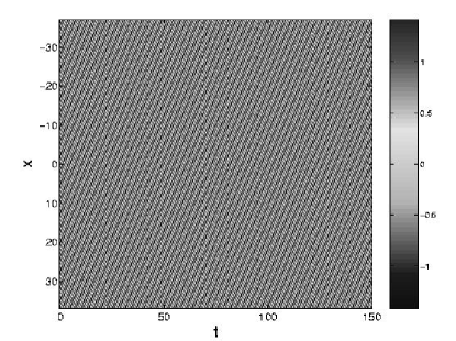
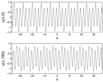
Figure 3: Same as Fig. 2 but for the periodic solution of the negative mKdV equation with $a=1$, $k=0.5$, $c=1.719$ and $m=0.057$ (such that $K(k)/a=2K(m)/c$). The dynamical evolution is stable.

4 Periodic Solution of the KdV Equation

Through the Miura transform $v=u^{2}\pm u_{x}$ [19] we can obtain the periodic solutions of the KdV equation ($v$) from the corresponding solutions of the negative mKdV equation ($u$). In particular, to the solution (19) of negative mKdV, corresponds the KdV solution of the form:

$$v=u^{2}+u_{x}=2\frac{[2\phi^{\prime 2}(x)-(1+\phi)\phi^{\prime\prime}(x)]}{(1-\phi^{2})(1+\phi)}\,,$$ (21)

where prime denotes derivative with respect to the argument. The other solution $u^{2}-u^{\prime}(x)$ is obtained from here simply by changing $\alpha$ to -$\alpha$. Using the solution (19) of the negative mKdV equation, we find that the solution (21) can be expressed in the form

$$v=\frac{2\alpha}{[1+\alpha\rm sn(ax+bt,k)\rm sn(cx+dt,m)]^{2}}\bigg{[}(a^{2}(1+k)+c^{2}(1+m))\rm sn(ax+bt,k)$$

$$\rm sn(cx+dt,m)+2a^{2}\alpha\rm sn^{2}(cx+dt,m)+2c^{2}\alpha\rm sn^{2}(ax+bt,k)$$

$$-2ac\rm cn(ax+bt,k)\rm dn(ax+bt,k)\rm cn(cx+dt,m)\rm dn(cx+dt,m)\bigg{]}\,.$$ (22)

Perhaps more interestingly, the Miura transform is an exact transformation between the solution of the negative mKdV equation ($\forall(x,t)$) and the one of the KdV equation. This implies that the numerically observed stability of the above mentioned lattice solution of the negative mKdV equation carries over to the existence and stability of such a solution in the setting of the KdV equation.

5 Conclusion

In this Letter, we have obtained new classes of periodic solutions for the positive and negative mKdV equations. The positive mKdV solutions (7) and (9) could be identified as the breather lattice and two-soliton lattice solutions, since in the appropriate limit they reduce to single breather and two-soliton solutions, respectively. In the case of the negative mKdV equation, lattice solutions have been identified in the form of Eqs. (16) and (19). However, the latter have not been designated as breather or soliton lattices (as the process of obtaining limiting expressions is less straightforward for the negative mKdV case).

We have also examined the stability of the various periodic solutions of mKdV equation with both positive and negative signs. We have found that the two-soliton lattice solution of the positive mKdV and the lattice solution (19) of the negative mKdV are quite robust with respect to perturbations in contrast with the breather lattice solution of the positive mKdV equation. These results, and more specifically the stability of the negative mKdV lattice solution, have direct implications for the corresponding lattice solutions of the KdV equation.

This work was supported in part by the U.S. Department of Energy. PGK is grateful to the Eppley Foundation for Research, the NSF-DMS-0204585 and the NSF-CAREER program for financial support.

References

References

- [1]
- [2] P.G. Drazin and R.S. Johnson, Solitons: an introduction (Cambridge University Press, Cambridge, U.K., 1989).
- [3] M.J. Ablowitz and H. Segur, Solitons and the Inverse Scattering Transform (SIAM, Philadelphia, 1981).
- [4] E. Infeld and G. Rowlands, Nonlinear Waves, Solitons and Chaos (Cambridge University Press, Cambridge, 1990).
- [5] R.K. Dodd, J.C. Eilbeck, J.D. Gibbon and H.C. Morris, Solitons and Nonlinear Waves (Academic Press, London, 1982).
- [6] A. Scott, Nonlinear Science (Oxford University Press, New York, 1999).
- [7] K. E. Lonngren, Optical and Quantum Electronics, 30, 615 (1998).
- [8] A. H. Khater, O. H. El-Kalaawy, and D. K. Callebaut, Phys. Script. 58, 545 (1998).
- [9] V. Ziegler, J. Dinkel, C. Setzer, and K. E. Lonngren, Chaos, Solitons and Fractals 12, 1719 (2001).
- [10] T. S. Komatsu and S. I. Sasa, Phys. Rev. E 52, 5574 (1995); T. Nagatani, Physica A 265, 297 (1999).
- [11] H. Ono, J. Phys. Soc. Jpn. 61, 4336 (1992).
- [12] W. K. Schief, Nonlinearity 8, 1 (1995).
- [13] M. Agop and V. Cojocaru, Mater. Trans. JIM 39, 668 (1998).
- [14] E. A. Ralph and L. Pratt, J. Nonlin. Sci. 4, 355 (1994).
- [15] S. Matsutani and H. Tsuru, J. Phys. Soc. Jpn. 60 (1991) 3640.
- [16] R.E. Goldstein and D.M. Petrich, Phys. Rev. Lett. 67, 3203 (1991); J. Langer and R. Perline, Phys. Lett. A 239, 36 (1998); K. S. Chou and C. Z. Qu, Physica D 162, 9 (2002).
- [17] P.G. Kevrekidis, A. Saxena, and A.R. Bishop, Phys. Rev. E 64, 026613 (2001).
- [18] P.G. Kevrekidis, A. Khare, and A. Saxena, Phys. Rev. E 68, 047701 (2003).
- [19] R. Miura, J. Math. Phys. 9, 1202 (1968).
- [20] Y. Ohta and R. Hirota, J. Phys. Soc. Jpn. 60, 2095 (1991).
- [21] M.J. Ablowitz and J.F. Ladik, J. Math. Phys., 16, 598 (1975); M.J. Ablowitz and J.F. Ladik, J. Math. Phys., 17, 1011 (1976).