Fano resonance in quadratic waveguide arrays

Abstract

We study resonant light scattering in arrays of channel optical waveguides where tunable quadratic nonlinearity is introduced as nonlinear defects by periodic poling of single (or several) waveguides in the array. We describe novel features of wave scattering that can be observed in this structure and show that it is a good candidate for the first observation of Fano resonance in nonlinear optics.

The study of nonlinear dynamics and spatial solitons in optical systems has recently attracted a great deal of attention book . In particular, many specific properties of nonlinear lattice systems can be analyzed for arrays of weakly coupled optical waveguides where both nonlinearity and diffraction may differ dramatically compared to those in the corresponding continuous systems review ; review2 .

During last years a growing interest is observed in the study of nonlinear optics associated with the so-called quadratic nonlinearities which may produce the effects resembling those known to occur in cubic nonlinear materials. Typical examples are all-optical switching phenomena in interferometric or coupler configurations as well as the formation of spatial and temporal solitons in planar waveguides buryak . Recently, it was demonstrated experimentally exp_chi2 that arrays of coupled channel waveguides fabricated in a periodically poled Lithium Niobate slab represent a convenient system to verify experimentally many theoretical predictions, including the first observation of two-frequency discrete solitons mutually locked by quadratic nonlinearity. These experimental observations open many perspectives for employing larger nonlinearities in lattice systems made of quadratic materials.

In this Letter we suggest to employ the arrays of weakly coupled nonlinear quadratic waveguides for the study of novel effects in resonant light scattering. In particular, we show that when periodic poling is applied to just a few waveguides in the array, it creates a nonlinear defect defect ; chi2_defect that possesses specific resonant scattering properties and may be employed for the first experimental observation of Fano resonance in nonlinear optics.

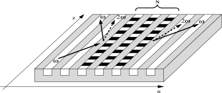
Figure 1: Schematic of an array of channel waveguides with quadratic nonlinearity where nonlinear defects are created by periodic poling. Arrows show the scattering process.

Following the waveguide design recently implemented in Ref. exp_chi2 for the observation of discrete quadratic solitons, we consider a discrete model describing an array of weakly coupled linear waveguides where one or several neighboring waveguides have periodic poling and therefore possess a quadratic nonlinear response (see Fig. 1). When the matching conditions are satisfied, the fundamental-frequency (FF) mode with the frequency $\omega$ can generate parametrically the second-harmonic (SH) wave at the frequency $2\omega$, so that such a structure with several poled waveguides may behave as a nonlinear defect with localized quadratic nonlinearity. The continuous version of this model has been studied earlier sukh_chi2 .

In the tight-binding approximation usually employed in the theory of discrete lattices review2 , the effective equations for the complex envelopes of the FF wave ($u_{n}$) and its SH component ($v_{n}$) coupled at the defect waveguides with $n=0,\ldots,N$ can be written in the dimensionless form

$$\begin{array}[]{l}{\displaystyle\mathrm{i}{du_{n}\over{dz}}+c_{u}(u_{n+1}+u_{n-1})+2\sum_{m=0}^{N}u_{m}^{*}v_{m}\delta_{nm}=0,}\\[9.0pt] {\displaystyle\mathrm{i}{dv_{n}\over{dz}}+c_{v}(v_{n+1}+v_{n-1})-\Delta v_{n}+\sum_{m=0}^{N}u_{m}^{2}\delta_{nm}=0,}\end{array}$$ (1)

where $c_{u}$ and $c_{v}$ are the coupling coefficients, $\delta_{nm}$ is the Kronecker symbol and $\Delta$ is the phase mismatch parameter assumed to be identical for all waveguides.

First, we analyze the scattering of a plane FF wave at the frequency $\omega$ by the a single ($n=0$) quadratic defect waveguide (‘impurity site’). After the interaction with the quadratic waveguide, the FF wave generates a SH wave which could either propagate or get trapped being guided by the defect waveguide. To calculate the transmission coefficient $t(k)$ of the FF wave, we present the fields in the form,

$$u_{n}(z)=\mathrm{exp}(\mathrm{i}\beta_{1}z)\left\{\begin{array}[]{ll}I\mathrm{exp}(\mathrm{i}kn)+R\mathrm{exp}(-\mathrm{i}kn)&\mbox{$n<0$}\\ T\mathrm{exp}(\mathrm{i}kn)&\mbox{$n\geq N$},\end{array}\right.$$ (2)

$$v_{n}(z)=\mathrm{exp}(\mathrm{i}\beta_{2}z)\left\{\begin{array}[]{ll}{\tilde{R}}\mathrm{exp}(-\mathrm{i}qn)&\mbox{$n<0$}\\ {\tilde{T}}\mathrm{exp}(\mathrm{i}qn)&\mbox{$n\geq N$},\end{array}\right.$$ (3)

where $\beta_{1}=2c_{u}\cos k$ and $\beta_{2}=2c_{v}\cos q-\Delta$ are propagation constants of the FF and SH respectively, and $k$ and $q$ are corresponding transverse wavenumbers. By using the phase-matching condition sukh_chi2 ($2\beta_{1}=\beta_{2}$) we obtain the relation $c_{v}\cos q-(\Delta/2)=2c_{u}\cos k$, that defines the dependence $q=q(k)$. For $k_{\rm min}<k<k_{\rm max}$, the function $q(k)$ takes real and positive values. Outside this interval, the values of $q(k)$ are purely imaginary, and they correspond to localized (non-radiating) states trapped by the defect waveguide at $n=0$. A simple calculation yields the result: $k_{\rm max,min}=\cos^{-1}[(c_{v}\pm\Delta/2)/2c_{u}]$, when these values are real and positive or zero, otherwise.

Evaluating the mode coupling at the impurity ($n=0$) and neighboring ($n=-1$) sites allows to obtain the relations, $T=I+R$ and ${\tilde{R}}={\tilde{T}}$, and derive a nonlinear equation for the transmission coefficient $t=|T|^{2}/|I|^{2}$ in the form, $t[1+b(k)t]^{2}=1$, where $b(k)=|I|^{2}\left[2c_{u}c_{v}\sin k\sin q(k)\right]^{-1}$, that has only one real solution. The resonant scattering, when a localized SH field is generated, can be analyzed similarly by replacing $q\rightarrow iq$.

The study of wave scattering in this system predicts the resonant suppression of transmission at some points, i.e. $t(k_{\rm min,max})=0$ (see Fig. 2). We demonstrate below that these resonant reflections correspond to a novel type of the well-known Fano resonance fano . Indeed, according to the Fano theory fano , destructive interference and resonant suppression of transmission are observed when there exists a localized state coupled to the propagating channel with the energy inside the linear spectrum. Note, that $q(k_{\rm min})=0$ and $q(k_{\rm max})=\pi$, i.e. these values define the band edges of the propagation spectrum of the propagating SH field, and the resonances take place when the SH field is generated. This situation seems to be in contradiction with the classical definition of the Fano resonance. However, below we demonstrate in more details that this kind of the resonant scattering can be indeed defined as being associated with the Fano resonance.

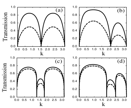
Figure 2: Examples of the FF transmission coefficient for the scattering by the quadratic impurity waveguide, for $c_{u}=1$, and (a) $c_{v}=0$, $\Delta=0$, (b) $c_{v}=0$, $\Delta=2$, (c) $c_{v}=0.5$, $\Delta=0$, and (d) $c_{v}=0.5$, $\Delta=2$, for two values of the intensity: $I=1$ (solid line) and $I=2$ (dashed lines).

First, we consider the simplest case when the coupling between the SH modes of different waveguides vanishes, i.e. $c_{v}=0$, which is indeed the case of the recent experiments exp_chi2 . Then, in the stationary case, the coupled equations (1) can be written in the form

$$\begin{array}[]{l}{\displaystyle\beta_{1}u_{n}=c_{u}(u_{n+1}+u_{n-1})+2u_{0}^{*}v\delta_{n0},}\\[9.0pt] {\displaystyle 2\beta_{1}v=-\Delta v+u^{2}_{0},}\end{array}$$ (4)

This model (4) describes the main propagation channel for the field $u_{n}$ and an additional discrete mode $v=v_{0}$ coupled to it parametrically, and it is similar to the so-called Fano-Anderson model mahan , except that the coupling here is nonlinear, that makes the scattering problem nonlinear.

To simplify the analysis, we eliminate the discrete mode described by the second equation and obtain,

$$\beta_{1}u_{n}=c_{u}(u_{n+1}+u_{n-1})+\frac{2|u_{0}|^{2}u_{0}}{2\beta_{1}+\Delta}\delta_{n0},$$ (5)

which is an effective equation for the propagation channel that contains a scattering potential. The strength of this nonlinear resonant scattering potential depends on the incoming intensity $|I|^{2}$ and propagation constant $\beta_{1}(k)$. If $\Delta$ is chosen such that $k_{F}$ is between $0$ and $\pi$, and

$$2\beta_{1}(k_{F})=-\Delta,$$ (6)

our potential becomes infinitely large for a particular frequency $\beta_{1}(k_{F})$, which will lead to the perfect reflection. Note here, that $k_{F}=k_{\rm min,max}$ for our case $c_{v}=0$. Indeed, after some algebra we can write down the equation for the transmission coefficient in the following form

$$t^{3}+\gamma(k)(t-1)=0,$$ (7)

where $\gamma(k)=(4c_{u}\cos k+\Delta)^{2}c_{u}^{2}\sin^{2}k/|I|^{4}$. From this equation one can see that, when $\gamma(k)=0$ then transmission coefficient $t$ vanishes. This happens at the wavenumbers $k=0$ and $k=\pi$, which correspond to the band edges of the propagation spectrum, and also at $k=k_{F}$. In the latter case, this is exactly the Fano resonance.

When the coupling between the SH modes in the waveguide array does not vanish (i.e. $c_{v}\not=0$), it leads to the appearance of the spectrum of propagating SH modes, $\beta_{2}[q(k)]$. At the band edges of this spectrum, $\beta_{2}(0)$ and $\beta_{2}(\pi)$, which correspond to $k=k_{\rm min}$ and $k=k_{\rm max}$, the propagating SH field is described as a standing constant-amplitude mode of the forms $v_{n}=v_{0}$ and $v_{n}=(-1)^{n}v_{0}$, respectively, where $v_{0}$ is constant. Therefore, for these two cases we can again obtain the single-site equation for the second scattering channel. By applying similar approach to these particular cases, we obtain two conditions for the Fano resonance,

$$2\beta_{1}(k_{F_{1,2}})=-\Delta\pm 2c_{v},$$ (8)

which occur exactly when the propagation constant $2\beta$ of the generated SH field coincides with either the propagation constant $\beta_{2}(0)$ or $\beta_{2}(\pi)$, i.e. at the band edges of the linear spectrum of the propagating SH modes. In other words, in such situations we excite ’constant modes’ by a local perturbation. Since the group velocity of these modes vanishes at the band edges, any local excitation could not propagate at the given frequency. It makes these modes effectively local and leads, finally, to the phenomenon of Fano resonance.

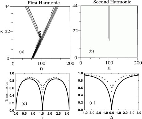
Figure 3: Top: Resonant generation of the trapped second-harmonic field by a Gaussian beam of the FF (a) and SH (b) fields for the parameters $c_{u}=1$, $c_{v}=0$, $\Delta=0$, and $k=\pi/2$. Bottom: Comparison of the transmission coefficients of the plane waves (solid) and Gaussian beam (crosses) for $c_{u}=1$, $c_{v}=0$ and (c) $\Delta=0$ and (d) $k=\pi/2$. Transmission coefficient of the Gaussian beam does not vanish due to its finite spectral width.

We note here that, in our physical system of quadratic waveguides, the coupling between the first and second propagation channels is nonlinear and, therefore, it depends on the intensity of the incoming wave. According to the formulas (6) and (8) the position of Fano resonances does not depend on the value of this coupling due to its local nature flach . As a consequence, this novel type of Fano resonance should exist for any intensity of incoming waves similar to the conventional Fano resonance in the linear theory. But the width of the resonance depends on this couplingaem and, therefore, on incoming intensity of light (see Fig. 2).

In order to check the validity of our plane wave analysis and the manifestation of the effect in a realistic experiment, we have performed the numerical simulation of the Gaussian beam scattering. The results are summarized in Fig. 3, and they are in a good agreement with the theory of plane wave scattering.

In the case of $N$ defects and vanishing coupling between them ($c_{v}=0$), Fano resonance does not change its position (6) periodic . After scattering by the first defect close to Fano resonance, other waveguides become almost transparent due to a small incoming intensity. Therefore, the width of the resonance will remain almost the same as in the case of a single defect.

In conclusion, we have analyzed a novel waveguide structure where an optical analog of the Fano resonance can be observed as peculiarities of the resonant scattering and second-harmonic generation in the quadratic waveguide arrays. We believe this kind of waveguide structures, already fabricated for the observation of discrete quadratic solitons exp_chi2 , is a good candidate for the first experimental observation of Fano resonances in nonlinear optics.

This work was partially supported by the Australian Research Council, a doctoral fellowship from Conicyt, and Fondecyt grants 1020139 and 7020139 in Chile. The authors thank Andrey Sukhorukov for useful discussions.

References

- (1) Yu.S. Kivshar and G.P. Agrawal, Optical Solitons: From Fibers to Photonics Crystals (Academic Press, San Diego 2003).
- (2) A.A. Sukhorukov, Yu.S. Kivshar, H.S. Eisenberg, and Y. Silberberg, IEEE J. Quantum Electron. 39, 31 (2003).
- (3) D.N. Christodoulides, F. Lederer, and Y. Silberberg, Nature 424, 817 (2003).
- (4) For a review, see A.V. Buryak, P. Di Trapani, D.V. Skryabin, and S. Trillo, Phys. Rep. 370, 63 (2002).
- (5) R. Iwanov, R. Schiek, G.I. Stegeman, T. Pertsch, F. Lederer, Y. Min, and W. Sohler, Phys. Rev. Lett. 93, 113902 (2004).
- (6) R. Morandotti, H.S. Eisenberg, D. Mandelik, Y. Silberberg, D. Modotto, M. Sorel, C.R. Stanley, and J.S. Aitchison, Opt. Lett. 28, 834 (2003).
- (7) C.B. Clausen and L. Torner, Phys. Rev. Lett. 81, 790 (1998).
- (8) A.A. Sukhorukov, Yu.S. Kivshar, and O. Bang, Phys. Rev. E 60, R41 (1999).
- (9) U. Fano, Phys. Rev. 124, 1866 (1961).
- (10) G.D. Mahan, Many-Particle Physics (Plenum, New York, 1993).
- (11) S. Flach, A.E. Miroshnichenko, V. Fleurov, and M.V. Fistul, Phys. Rev. Lett. 90, 084101 (2003).
- (12) A. E. Miroshnichenko, S. Flach, and B. Malomed, Chaos 13, 874 (2003).
- (13) D. W. L. Sprung, H. Wu, and J. Martorell, Am. J. Phys. 61, 1118 (1993).