$1/f^{\alpha}$ spectra in elementary cellular automata and fractal signals

Abstract

We systematically compute the power spectra of the one-dimensional elementary cellular automata introduced by Wolfram. On the one hand our analysis reveals that one automaton displays $1/f$ spectra though considered as trivial, and on the other hand that various automata classified as chaotic/complex display no $1/f$ spectra. We model the results generalizing the recently investigated Sierpinski signal to a class of fractal signals that are tailored to produce $1/f^{\alpha}$ spectra. From the widespread occurrence of (elementary) cellular automata patterns in chemistry, physics and computer sciences, there are various candidates to show spectra similar to our results.

In 1984 Wolfram introduced the so-called elementary cellular automata (ECA), opening a field still being vividly active 20 years thereafter wolfram . Wolfram’s more recent popular book nks has attracted great attention, although the opinion of the work’s merits are divided among the scientific community nks_review . ECA are discussed extensively in the context of computationally irreducibility of physical systems israeli2004 , e.g. it is proven that in the Turing sense herken1995 rule 110 (being one of the possible 256 ECA) is an universal computer wolfram . Moreover, possible transformations between difference equations and (E)CA have been investigated nobe2001 . Among the numerous physical applications we mention here only (kinetic phase transitions in) catalytic reaction-diffusion systems ziff1986 ; dress84plath ; hayase ; claussen2004 , deterministic surface growth krug1988 , branching and annihilating random walks cardy1997 and random boolean networks matache2004 .
It is important to note that Wolfram’s ECA are often studied for different boundary conditions on a finite array. A particular boundary condition (e.g. a periodic or an absorbing one) disturbs the pure evolution of an ECA. As a result, some automata display complex behavior, while other are simply periodic. Though there is no algorithm for classifying a given elementary automaton, Wolfram conjectured that ECA can be grouped into four classes of complexity:
Class 1: Steady state, class 2: Periodic or nested structures, class 3: Random (chaotic) behavior, class 4: Mixture of random and periodic behavior.

The first class represents automata that are (for almost all initial conditions) trivial in the sense being static or finally evolve to the some steady state. Those rules that belong to the second class produce simple periodic or self-similar, i.e. fractal, structures. The third class includes rules exhibiting random patterns, e.g. a particular rule (number 30) is used to generate random numbers in Mathematica. The fourth class is somehow a mixture of classes 2 and 3 generating the most complex structures. For more rigorous classifications we refer the reader to the literature barbosa2004 ; israeli2004 .

Since the coining paper of Bak, Tang, and Wiesenfeld btw , there has been considerable interest in the long-time behavior of cellular automata, especially for occurrence of long range correlations, and correspondingly for power spectra exhibiting a power law decay $S(f)\sim f^{-\alpha}$ with $\alpha\approx 1.0$. Despite the abundance in nature, systems exhibiting spectra with exponents near to 1 are poorly understood. While the mechanisms generating $1/f^{\alpha}$ spectra may be substantially different from each other, some models and the observed $1/f^{\alpha}$ power laws have become a paradigm for complex dynamical systems in general jensen (see also references in claussen2004 ).

Definition of ECA.

An elementary cellular automaton consists of an infinite one-dimensional lattice of cells being either black (1) or white (0), and a deterministic update rule. At each discrete time step, a cell is updated $x_{n}^{t}\rightarrow x_{n}^{t+1}$ according to the state of the next-neighbor sites and its own state one time step before:

$$x_{n}^{t+1}=f(x_{n+1}^{t},x_{n}^{t},x_{n-1}^{t})$$ (1)

where $f$ (the rule) is determined by $8$ bits being the output of the possible input bits $000$, $001$, …, $111$. As a consequence, there are 256 (ECA-)rules that are named rule 0 - 255. In this article we focus on rules 90 and 150 defined by

$$x_{n}^{t+1}=[x_{n-1}^{t}+rx_{n}^{t}+x_{n+1}^{t}]~{}{\rm{}mod}~{}2$$ (2)

where $r=0$ defines rule 90, and $r=1$ rule 150, respectively. As demonstrated earlier, rule 90 can be interpreted in the context of catalytic processes. A process (catalysis) is initiated (or continued) when exactly 1 neighbor site is active whereas the process (catalysis) is stopped when too many, i.e. 2, or to less, i.e. no, neighbor sites are active claussen2004 .

A similar interpretation may be given for rule 150. Catalysis at $x_{n}^{t}$ is stopped when no or two neighbor sites (now $x_{n}^{t}$ included) are active and it is initiated (or continued) when one or three sites are active. Note that both rules mimic local self-limiting reaction processes dress84plath ; otterstedt98 .

Spectra of sum signals.

It is known that ECA on finite lattices for various boundary conditions display no $1/f^{\alpha}$ spectra wolfram . Rather than evaluating the rules on finite lattices we calculate the evolution on an infinite lattice. More precisely, we focus on a sum signal defined as the total (in)activity, magnetization, etc. of the whole system:

$$X(t)=\sum_{n}x_{n}^{t}.$$ (3)

We have systematically investigated all 256 rules, for localized initial conditions (i.e. single 1, 11, 101, 111, …), as follows. The sum signal for non-trivial rules exhibits increasing mean $\langle X\rangle_{t}$ well fitted by a power law in time . Consequently, we focus on the detrended sum signal defined by

$$Y(t)=X(t)-f(t)$$ (4)

where the coefficients of $f(t)=at^{b}$ are fitted. However for some ECA $Y(t)$ possesses an increasing mean variance. Thus we investigate for each automaton another signal (and its spectrum)

$$Z(t)=Y(t)/\langle Y\rangle_{\{t-l+1,t+l\}}^{1/2}$$ (5)

where $2l$ is the width of a sliding window that normalizes the fluctuations of the detrended signal $Y(t)$ according to the method of detrended fluctuation analysis (DFA) applied for non-equilibrium processes hu2001 . We have calculated the corresponding power spectra $|X(\omega)|^{2}$, $|Y(\omega)|^{2}$ and $|Z(\omega)|^{2}$ for all 256 ECA. It turns out that that 25 of the 256 rules exhibit $1/f^{\alpha}$ spectra whereas 231 do not (see table 1). 23 of those automata that exhibit $1/f^{\alpha}$ spectra display Sierpinski patterns, i.e. well studied self-similar structures claussen2004 . Their spectra are extensively investigated in claussen2004 exhibiting $1/f^{\alpha}$ spectra with exponents $1.15\pm 0.05$.

Class	ECA rule number
1	218
2	(26, 82, 167, 181), (154, 210)
3	(18, 183), (22, 151), (60, 102, 153, 195), (90, 165),
	(122, 161), (126, 129), (146, 182), 105, 150
4	-

Table 1: Rules that produce $1/f^{\alpha}$ spectra. Rules in brackets belong to one equivalence class. Rules 105 and 150 (bold) produce spectra with power law exponents about $\alpha=1.3$. All other listed rules exhibit spectra with exponents about $\alpha=1.2$. The 231 rules not listed are not capable to produce $1/f^{\alpha}$ spectra, e.g. most of the spectra display no power law decay, or exhibit thermal $1/f^{2}$ spectra (see Fig. 2).

The two other rules, i.e. 105 and 150, show a different behavior. Here we focus on rule 150 . The first 128 time steps of the evolution for a single 1 as initial condition is depicted in Fig. 1 (upper inset).

Figure 1: The first 128 time steps of the time signal $X(t)$ generated by rule 150. Upper Inset: Self-similar structure generated by rule 150 for the first 64 time steps. Lower Inset: Normalized signal $Z(t)$; the straight line indicates $Z=0$.

It is a Sierpinski-like self-similar structure. However the fractal dimension differs from the Sierpinski gasket ($d=1.58$) being the golden mean $d=(1+\sqrt{5})/2\approx 1.69$. Fig. 1 shows also the corresponding signals $X(t)$ and $Z(t)$. The spectrum $Y(\omega)$ is displayed in Fig. 2. For $\omega$ not too small, the averaged spectrum exhibits a straight line in the log-log-plot verifying a power law behavior. Depending on the average process and fit range we obtain a fit exponent of about $\alpha=1.27\pm 0.05$. Due to dominating randomness, members of classes 3 and 4 typically produce thermal $1/f^{2}$ spectra (see Fig. 2).

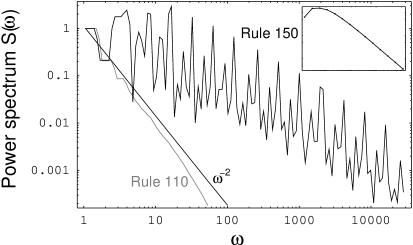
Figure 2: Rule 150 and rule 110: Averaged power spectrum of $Y(t)$ up to $T/8$ for $T=2^{18}$ using (incommensurable) $1.1^{k}$-bins, i.e.  the $k$-th interval is defined by $[\lceil 1.1^{k}\rceil,\lceil 1.1^{k+1}\rceil]$ where the brackets $\lceil~{}\rceil$ denote upwards rounded integer values (ceiling function). The inset shows the rule 150 spectrum, averaged using $2^{k}$-bins, i.e. the $k$-th interval is defined by $[2^{k},2^{k+1}-1]$. Both averages correspond to a constant $\delta\omega/\omega$ ratio. The graphs are well fitted by a power law with exponent $\alpha=1.27$. The thermal $1/f^{2}$ decay of rule 110 (grey) as a typical member of Class 4 is shown for comparison.

Fractal signals produce $1/f^{\alpha}$ spectra.

All ECA that are capable to produce a self-similar structure exhibit $1/f^{\alpha}$ spectra. Hence one may naively expect that every (self-similar) fractal structure produces $1/f^{\alpha}$ spectra. However it is important to note that this is not the case. There are many fractals like the Koch snow flake, Cantor dust etc. exhibiting no $1/f^{\alpha}$ spectra  because their respective sum signals simply grow exponentially mandelbrot .
Rather than a geometric approach we focus on fractal signals itself. Thus we now generalize the recently investigated Sierpinski signal claussen2004 . As we will see, the generalized signal is capable to model $1/f^{\alpha}$ spectra producing spectra with continuously tunable power law exponents. More precisely, we consider the signal

$$X_{\delta}(t)=2^{\delta\sum_{j}\sigma_{j}\{t\}}$$ (6)

where $\sigma_{j}$ is the $j$th bit of the binary decomposition of the discrete time $t=0,1,2,...$. For $\delta=1$ we have shown recently both numerically and analytically that the signal exhibits $1/f^{\alpha}$ spectra with $\alpha$ close to unity. The special ansatz, eq. (6), represents a straightforward generalization of the closed form for the sum signal of the Sierpinski pattern produced by rule 90 claussen2004 . In the next paragraph we show that for deviations from $\delta=1$ the signal can produce $1/f^{\alpha}$ spectra within a wide range of exponents $\alpha$.
In analogy to the calculation in Ref. claussen2004 , we calculate the periodogram $X(\omega)$ of the time signal (6) analytically:

$$X(\omega) = \sum_{t=0}^{2^{N}-1}{\rm{}e}^{{\rm{}i}\omega t}X_{\delta}(t)$$ (7)

$$= \sum_{\{\sigma_{0},\ldots,\sigma_{N-1}\}}\exp({\rm{}i}\omega\sum_{j}\sigma_{j}2^{j})~{}X_{\delta}(\sum_{j}\sigma_{j}2^{j})$$

$$= \sum_{\{\sigma_{0},\ldots,\sigma_{N-1}\}}\prod_{j=0}^{N-1}\exp\left(\sigma_{j}({\rm{}i}\omega 2^{j}+\delta\ln 2)\right)$$

$$= \prod_{j=0}^{N-1}\sum_{\{\sigma_{j}\}}\exp\left(\sigma_{j}({\rm{}i}\omega 2^{j}+\delta\ln 2)\right)$$

$$= \prod_{j=0}^{N-1}\left(1+\exp({\rm{}i}\omega 2^{j}+\delta\ln 2)\right).$$

The absolute value of $X(\omega)$ simplifies to a trigonometric product which the logarithm converts into a sum:

$$\ln|X(\omega)|^{2}=\sum_{j=0}^{N-1}\ln[1+2^{2\delta}+2^{1+\delta}\cos(\omega 2^{j})].$$ (8)

We roughly estimate the sum in eq. (8) replacing the sum by an integral, and substituting $y=\omega 2^{j}$,

$$\ln|X(\omega)|^{2} \approx \int_{0}^{N-1}\ln[1+2^{2\delta}+2^{1+\delta}\cos(\omega 2^{j})]{\rm d}j$$ (9)

$$= \int_{\omega}^{\omega 2^{N-1}}\frac{\ln[1+2^{2\delta}+2^{1+\delta}\cos y]}{y\ln 2}{\rm d}y.$$ (10)

As $\ln(a+bx)\approx\ln(a)+\frac{b}{a}x$ for $|x|\ll 1$, we obtain

$$\ln|X(\omega)|^{2}\approx\frac{\ln(1+2^{2\delta})}{\ln 2}\!\int_{\omega}^{\omega 2^{N-1}}\!\!\frac{{\rm d}y}{y}+$$

$$\frac{2^{1+\delta}}{(1+2^{2\delta})\ln 2}\!\int_{\omega}^{\omega 2^{N-1}}\!\!\frac{\cos(y)}{y}{\rm d}y.$$ (11)

The integral over the integral cosine is nearly independent of the upper boundary for high values of the boundary. Thus, we can substitute the upper boundary $\omega 2^{N-1}$ by some $N$-dependent constant, say $c_{N}\gg 1$. Finally, replacing the cosine by one yields immediately a rough approximation of the power spectrum:

$$|X(\omega)|^{2}\approx c_{N}^{\prime}\omega^{-\frac{2^{1+\delta}}{(1+2^{2\delta})\ln 2}}.$$ (12)

For a given power law exponent $0<\alpha\leq 1/\ln 2\approx 1.44$, we obtain $\delta$ from eq. (12) as

$$\delta=\frac{\ln\Big{(}\frac{1+\sqrt{1-\alpha^{2}(\ln 2)^{2}}}{\alpha\ln 2}\Big{)}}{\ln 2}.$$ (13)

To generate signals with goal exponents, e.g., $\alpha_{1}=0.8,\alpha_{2}=1.0,\alpha_{3}=1.2$, one can use the corresponding value of $\delta$ according to Eq. (13). Fig. 3 shows the spectrum of the detrended signal (6) for $\delta_{2}=1.31184$ (corresponding to $\alpha_{2}=1.0$). For $\delta_{1}=1.72425$ and $\delta_{3}=0.902749$ the individual spectra exhibit similar graphs (not shown). Depending on the averaging the power law fits giving $\alpha_{1}=0.8\pm 0.1$, $\alpha_{1}=0.95\pm 0.05$ and $\alpha_{3}=1.2\pm 0.05$, are in good agreement with the theoretical results.

Figure 3: Averaged power spectrum of the detrended signal (6) for $\delta=1.31184$ up to $T/8,~{}T=2^{20}$ using (incommensurable) $1.1^{k}$-bins, i.e. the $k$-th interval is defined by $[\lceil 1.1^{k}\rceil,\lceil 1.1^{k+1}\rceil]$ where the brackets $\lceil~{}\rceil$ denote upwards rounded integer values (ceiling function). The inset shows the spectrum, averaged using $2^{k}$-bins, i.e. the $k$-th interval is defined by $[2^{k},2^{k+1}-1]$. Both correspond to a constant $\delta\omega/\omega$ ratio possessing fit exponents of about $\alpha=0.93$. The corresponding spectrum for the variance detrended signal exhibits power spectra around $\alpha=1.0$. The theoretical exponent is $\alpha=1.0$.

Two-dimensional automaton.

While one-dimensional experimental setups as in otterstedt98 seem to be quite artificial for (self-limiting) catalytic processes, two-dimensional dynamics is more generic. Consider the Sierpinski dynamics on a $(i,j)$-plane:

$$x_{i,j}^{t+1}=[x_{i+1,j}^{t}+x_{i-1,j}^{t}+x_{i,j+1}^{t}+x_{i,j-1}^{t}]~{}{\rm{}mod}~{}2.$$ (14)

For a single 1 as initial condition on a plane the sum signal $X_{2D}(t)=\sum_{i,j}x_{i,j}^{t}$ generates the sequence

$$X_{2D}(t)=1,4,4,16,4,16,16,64,\ldots$$ (15)

More precisely, the recurrence relation generating eq. (15) is given by $u_{n}\rightarrow u_{n+1}=(u_{n},4u_{n})$ for $u_{0}=(1)$.
First, if the factor 4 is replaced by 2, the relation becomes equivalent to the 1d-Sierpinski signal $X_{1D}(t)$ in Ref. claussen2004 . Second, we obtain $X_{2D}(t)=X_{1D}(t)^{2}$ and therefore $X_{2D}(t)=X_{\delta=2}(t)$. Thus the generalized Sierpinski pattern in two dimensions exhibits $1/f^{\alpha}$ spectra with exponents around the value according to eq. (12) for $\delta=2$, that is $\alpha=0.679$. We numerically verified the value obtaining exponents around $\alpha=0.7$ as expected.

Conclusions.

Elementary Cellular automata are a paradigm for emergence of complex spatiotemporal behavior from extremely simple dynamics. We systematically investigated all 256 elementary cellular automata. As expected, among those as (nested) periodic/chaotic classified rules (classes 2 and 3) there are various rules that display $1/f^{\alpha}$ spectra (see table 1). Unexpectedly, on the one hand all rules classified as complex display no $1/f^{\alpha}$ spectra, while on the other hand, the trivial rule 218 does (being a member of class 1). It is important to note that the numerically calculated spectra are robust against noise, that is, the fit exponents change only slightly for other initial conditions than a single seed.
Moreover we generalized the approach of a sum signal introduced in claussen2004 to derive analytically the spectra of the 2D Sierpinski automaton. The investigated fractal signals (6) serve also as a fit model for signals produced by elementary cellular automata rules. We have obtained a time series generator with continuously tunable power law decay exponent. The tailored signals represent analytically tractable (nontrivial) $1/f^{\alpha}$ generators that shed light on the arcane mechanisms of $1/f^{\alpha}$ spectra.
From our results, we expect that in experimental systems showing spatiotemporal pattern formation similar to the ECA patterns, the power spectra of the total (in)activity will exhibit power law behavior within a certain range.

References

- (1) S. Wolfram, Physica D 10, 1-35 (1984); Nature 311, 419 (1984); Rev. Mod. Phys. 55, 601 (1983).
-
(2)
S. Wolfram,
A New Kind of Science, (2002).
http://www.wolframscience.com/nksonline/toc.html. - (3) News feature, Nature 417, 216, (2002).
- (4) Navot Israeli and Nigel Goldenfeld, Phys. Rev. Lett. 92, 074105 (2004); Phys. Rev. Focus 13, story 10 (2004).
- (5) The Universal Turing Machine, A Half-Century Survey, edited by R. Herken (Springer-Verlag, Wien, 1995).
- (6) Nobe A., Satsuma J. and Tokihiro T., J. Phys. A 34, L371-L379 (2001).
- (7) Robert M. Ziff, Erdagon Gulari, and Yoav Barshad, Phys. Rev. Lett 56, 2553, (1986).
- (8) Y. Hayase, J. Phys. Soc. Jpn. 66, 2584 (1987); Y. Hayase and T. Ohta, Phys. Rev. Lett. 81, 1726 (1998); Y. Hayase and T. Ohta, Phys. Rev. E 62, 5998 (2000).
- (9) A. W. M. Dress, M. Gerhardt, N. I. Jaeger, P. J. Plath, H. Schuster, in: L. Rensing and I. Jaeger (eds.), Temporal Order, Springer, Berlin (1984).
- (10) Jens Christian Claussen, Jan Nagler, and Heinz Georg Schuster, Phys. Rev. E 70, 032101 (2004).
- (11) J. Krug, H. Spohn, Phys. Rev. A 38, 4271, (1988).
- (12) John Cardy, and Uwe C. Täuber, Phys. Rev. Lett. 77, 4780, (1996).
- (13) Mihaela T. Matache, and Jack Heidel, Phys. Rev. E 69, 056214, (2004).
- (14) V. C. Barbosa, F. M. N. Miranda, M. C. M. Agostini, nlin.CG/0408014, (2004).
- (15) P. Bak, C. Tang, and K. Wiesenfeld, Phys. Rev. Lett. 59, 381 (1987), Phys. Rev. A 38, 364 (1988).
- (16) H. J. Jensen, Self-Organized Criticality, Cambridge Univ. Press (1998).
- (17) R. D. Otterstedt, N. I. Jaeger, P. J. Plath, and J. L. Hudson, Phys. Rev. E 58, 6810-6813 (1998).
- (18) K. Hu, P.C. Ivanov,, Z. Chen, P. Carpena, and H.E. Stanley, Phys. Rev. E, 64, 011114, (2001).
- (19) Benoit B. Mandelbrot, Multifractals and 1/f noise, Springer (1999); Benoit B. Mandelbrot, Fractals and chaos, Springer (2004).