Polymer transport in random flow

Abstract

The dynamics of polymers in a random smooth flow is investigated in the framework of the Hookean dumbbell model. The analytical expression of the time-dependent probability density function of polymer elongation is derived explicitly for a Gaussian, rapidly changing flow. When polymers are in the coiled state the pdf reaches a stationary state characterized by power-law tails both for small and large arguments compared to the equilibrium length. The characteristic relaxation time is computed as a function of the Weissenberg number. In the stretched state the pdf is unstationary and exhibits multiscaling. Numerical simulations for the two-dimensional Navier-Stokes flow confirm the relevance of theoretical results obtained for the $\delta$-correlated model.

• Polymer transport in random flow

• Dario Vincenzi
  CNRS, Observatoire de la Côte d’Azur
  Bd. de l’Observatoire B. P. 4229
  06304 Nice Cedex 4, France

• +33-4-92003172

• +33-4-92003121

• Dario.Vincenzi@obs-nice.fr

To be published in the Journal of Statistical Physics

KEY WORDS: Elastic dumbbell model; Coil-stretch transition; Turbulent transport; Batchelor-Kraichnan statistical ensemble.

1 Introduction

A polymer is a long, repeating chain formed through the linkage of many identical smaller molecules called monomers. Understanding the behavior of a single polymeric chain passively advected by a turbulent flow is the first step in the study of polymer transport. At equilibrium a polymer molecule coils itself up into a ball of radius $R_{0}$. When placed in a non-homogeneous flow, the polymer deforms and stretches; if the number of monomers composing the molecule is large, the end-to-end distance of the polymer, $R$, can become much greater than the equilibrium size $R_{0}$. A sharp transition from the coiled state to the strongly stretched one is observed when the strain rate exceeds a critical value [1, 2].

Two competing effects determine the deformation of a polymer: the stretching by the velocity gradients and the elastic relaxation towards the equilibrium shape. Theoretical and numerical results suggest that a wide range of scales exists where the elasticity of the polymer can be described by Hooke’s law [3]. In the absence of flow the configuration of the polymer converges exponentially to the equilibrium shape: $R\approx R_{0}\,e^{-t/\tau}$, where $\tau$ is the characteristic time of the slowest oscillation mode. In contrast, a non-homogeneous velocity field can stretch the polymer and elongate it. The characteristic value of velocity gradients is determined by the maximum Lyapunov exponent $\lambda$, which is the average logarithmic growth rate of fluid particle separations (see, e.g., ref. [4]).

In random flows the ratio of the relaxation time to the characteristic stretching one is determined by the Weissenberg number $\text{Wi}\equiv\lambda\tau$. When $\text{Wi}<1$ contraction is faster and the extension of the molecule converges definitively to the equilibrium size; the polymer, therefore, is in the coiled state. When $\text{Wi}>1$ the elastic force is weak and the velocity gradients can deform considerably the molecule. In this case the dynamics of the polymer depends strongly on the properties of the advecting flow. Balkovsky et al. have shown that in random flows the threshold $\text{Wi}=1$ marks the coil-stretch transition and polymers are highly stretched when Wi exceeds one [5, 6]. Only very recently has the coil-stretch transition in random flows been observed experimentally by Gerashchenko et al. [7]. It should be however noted that there can be particular flows where the coil-stretch transition never occurs. This generally happens when a strong rotation prevents the molecules from getting aligned with the stretching direction [8].

When polymers are highly stretched the coupling between elastic and kinetic degrees of freedom should be taken into account. The feedback on the advecting flow is then modeled by an additional term in the stress tensor appearing in the Navier-Stokes equations. The most important effect of the back reaction on the velocity field is probably the drag reduction (see, e.g., ref. [9]). The passive approach, however, is justified when the stress due to polymers is much smaller than the viscous stress, which can be estimated as $\nu_{v}\lambda$, $\nu_{v}$ being the kinematic viscosity of the fluid [5, 6].

We focus on passive polymer transport: the velocity field is given and reaction effects on the advecting flow are neglected. We study the coil-stretch transition when the extension of polymers is much smaller than their maximum length $R_{max}$ and the correlation time of the velocity field is negligible. The polymer is modeled by a Hookean elastic dumbbell and the turbulent advecting flow belongs to the Batchelor-Kraichnan statistical ensemble [10, 11]. The same model was previously investigated by Chertkov [12] and Thiffeault [13]. Chertkov derived an approximate equation for the right tail of the probability density function (pdf) of the end-to-end separation of the dumbbell [12]. Thiffeault obtained asymptotic results for the stationary solution of this equation in three dimensions [13]. We derive the Fokker-Planck equation for the complete pdf of the end-to-end distance of the polymer in general dimension $d$. We thus obtain the exact stationary form and the finite-time behavior of the pdf of the elongation. Finally, we compare theoretical results with numerical simulations for the two-dimensional Navier-Stokes flow.

The rest of this paper is organized as follows. Section 2 is devoted to the description of the model. In Section 3 we derive the Fokker-Planck equation for the probability density function of the extension $R$. The stationary solution and the finite time pdf are discussed in Section 4 and in Section 5 respectively. In Section 6 we discuss the results of numerical simulations of polymer dynamics in the two-dimensional Navier-Stokes flow. Section 7 is reserved to conclusions.

2 Elastic dumbbell model

A simple description of the complex structure of polymers is provided by Rouse’s model, which represents a polymer as a chain of $N$ beads connected by Hookean springs [14]. The dynamics can be solved by decomposing the motion of the molecule into a set of linear normal modes. A typical relaxation time is associated with the amplitude of each mode. In many physical applications the dynamics of the polymer is dominated by the fundamental mode, whose relaxation time is of the order of $\zeta/k$, where $\zeta$ is the friction coefficient of the polymer and $k$ is the spring constant.

The elastic dumbbell model is a simplification of Rouse’s model. Only the fundamental oscillation mode is taken into account and the elasticity of the polymer is modeled by a single spring connecting the ends of the molecule. Two beads of radius $l$ are joined at their centers by a linear zero-length spring of stiffness $k$. For a chain of $N$ identical monomers of length $L$ the spring constant is $k=3KT/(N-1)L^{2}$, where $K$ is the Boltzmann constant and $T$ the temperature [15]. The positions of the beads are defined by the vectors $\bm{x}_{1}$ and $\bm{x}_{2}$; the two beads represent the ends of the polymer and their separation $\bm{R}=\bm{x}_{2}-\bm{x}_{1}$ determines the elongation of the molecule (fig. 1). The idea of using a dumbbell to simulate a polymer dates back to Kuhn [16]. For the sake of completeness, we review the derivation of the governing equation for the bead connector (see, e.g., ref. [17]).

The hydrodynamic drag force that one bead experiences due to its relative motion to the fluid is given by Stokes’ law: $-\zeta[\dot{\bm{x}}_{i}-\bm{v}(\bm{x}_{i},t)]$, where $\dot{\bm{x}}_{i}$ is the velocity of the bead $i$ and $\bm{v}(\bm{x}_{i},t)$ the velocity of the fluid at the position of the bead. The friction coefficient is $\zeta=6\pi l\eta_{v}$, where $\eta_{v}$ denotes the dynamical viscosity of the solvent.

The size of the beads is assumed to be small enough for their dynamics to be influenced by thermal noise. This is modeled by a Gaussian process $\sqrt{2\zeta KT}\,\bm{\xi}_{i}$ such that [18]

$$\langle\bm{\xi}_{i}(t)\rangle=0\qquad\langle\xi^{k}_{i}(t)\,\xi_{j}^{\ell}(t^{\prime})\rangle=\delta_{ij}\delta^{k\ell}\delta(t-t^{\prime})\qquad(i,j=1,2)$$ (1)

Owing to molecular noise the equilibrium size of the dumbbell is not zero, but it can be estimated as $R_{0}=\sqrt{KT/k}$ by considering the elastic energy of the polymer, $E=kR^{2}/2$, and its equilibrium value at temperature $T$, $E=KT/2$.

Taking into account the elastic force, the hydrodynamic drag, and the thermal noise, we obtain the dynamical equations for the beads:

$$\begin{array}[]{c}m\ddot{\bm{x}}_{1}=-k\left(\bm{x}_{1}-{\bm{x}}_{2}\right)-\zeta\,\left[\dot{\bm{x}}_{1}-\bm{v}(\bm{x}_{1},t)\right]+\sqrt{2\,\zeta KT}\,\bm{\xi}_{1}\\[8.5359pt] m\ddot{\bm{x}}_{2}=-k\left(\bm{x}_{2}-{\bm{x}}_{1}\right)-\zeta\,\left[\dot{\bm{x}}_{2}-\bm{v}(\bm{x}_{2},t)\right]+\sqrt{2\,\zeta KT}\,\bm{\xi}_{2}\end{array}$$ (2)

In physical applications the elongation of the polymer, however large it is, never reaches the viscous scale of the turbulent flow, where dissipation and advection balance [19]. Below this scale velocity fluctuations are attenuated by the viscosity and the flow is smooth. Thus, during its evolution the polymer always moves in a regular velocity field, which at the scale $R$ can be approximated by a uniform gradient flow [10]:

$$\bm{v}(\bm{x}_{2},t)=\bm{v}(\bm{x}_{1},t)+(\bm{x}_{2}-\bm{x}_{1})\cdot\nabla\bm{v}(t)$$

Neglecting inertial effects, we finally derive from (2) a stochastic ordinary differential equation for the end-to-end separation of the polymer [17]:

$$\dot{\bm{R}}=(\bm{R}\cdot\nabla)\bm{v}-\frac{\bm{R}}{\tau}+\sqrt{\frac{2R_{0}^{2}}{\tau}}\;\bm{\xi}$$ (3)

where $\tau=\zeta/2k$ is the relaxation time and $\bm{\xi}\equiv(\bm{\xi}_{2}-\bm{\xi}_{1})/\sqrt{2}$ has the same properties as $\bm{\xi}_{1}$ and $\bm{\xi}_{2}$ [see eq. (1)]. Equation (3) governs the dynamics of the elongation of a polymer transported by a non-homogeneous flow: the velocity gradients stretch the molecule, which reacts elastically and attempts to recover the equilibrium spherical shape. Thermal fluctuations of the solvent are modeled by the white noise $\sqrt{2R_{0}^{2}/\tau}\,\bm{\xi}$.

It should be noted that the infinitely extensible dumbbell is a good approximation of a polymer only when the extension of the molecule is much smaller than its maximum length $R_{max}$. For very large elongations ($R\lesssim R_{max}$) the relaxation time becomes a function of $R$ and the resulting elastic force is nonlinear [3]. In more realistic dumbbell models, Hooke’s law is replaced by a force diverging as the size of the polymer approaches $R_{max}$ (for the description of the dynamics of a FENE dumbbell transported by the Batchelor-Kraichnan flow see refs. [13, 21]). Our results thus apply to the range $R\ll R_{max}$.

3 Fokker-Planck equation

The probability density function of the elongation, $P(\bm{R},t)$, obeys the Fokker-Planck equation associated with eq. (3) (see, e.g., refs. [18, 22])

$$\frac{\partial P}{\partial t}+\frac{\partial}{\partial R^{i}}\left(R^{j}\nabla^{j}v^{i}-\frac{R^{i}}{\tau}\right)P=\frac{R_{0}^{2}}{\tau}\frac{\partial^{2}P}{\partial R^{i}\partial R^{i}}$$ (4)

where summation over repeated indices is understood. In the passive regime the turbulent advecting flow has to be specified. Within the context of Kraichnan’s model, $\bm{v}$ is a Gaussian random field with zero mean and correlation function [11]

$$\langle v^{i}(\bm{x},t)\,v^{j}(\bm{x}+\bm{r},t^{\prime})\rangle={\mathscr{D}}^{ij}(\bm{r})\,\delta(t-t^{\prime})$$

The velocity field is by definition statistically homogeneous in space and stationary in time. The non-realistic property of the Kraichnan ensemble is the $\delta$-correlation in time, which defines a stochastic process with no memory. Nevertheless, the absence of time correlation in the advecting flow yields closed equations for the correlation functions of the transported field. The study of this model brought important results in turbulent transport theory; these can be interpreted as the limit of real behaviors as the velocity correlation time tends to zero (see ref. [4] for a review). A complete definition of Kraichnan’s model requires writing the covariance tensor ${\mathscr{D}}^{ij}(\bm{r})$ explicitly. If we impose incompressibility, smoothness, and statistical invariance under parity and rotations, ${\mathscr{D}}^{ij}(\bm{r})$ takes the form [23]

$${\mathscr{D}}^{ij}(\bm{r})=D_{0}\delta^{ij}-D_{1}[(d+1)\delta^{ij}r^{2}-2r^{i}r^{j}]$$

where the constant $D_{0}$ is the eddy diffusivity of the flow, $D_{1}$ determines the intensity of the fluctuations of the velocity, and $d$ is the physical dimension of the flow ($d=2,3$ in practical applications). Consequently, the two-time correlation of the velocity gradients takes the form

$$\langle\nabla^{i}v^{j}(t)\,\nabla^{k}v^{\ell}(t^{\prime})\rangle=2D_{1}[(d+1)\delta^{ik}\delta^{j\ell}-\delta^{ij}\delta^{k\ell}-\delta^{i\ell}\delta^{jk}]\,\delta(t-t^{\prime})$$ (5)

It is worth noticing that when $\bm{v}$ is a Gaussian white noise the advection term in eq. (3) defines a multiplicative stochastic process like the ones considered in refs. [24, 25, 26, 27].

By averaging eq. (4) over realizations of the velocity field, we obtain the evolution equation for the average probability density function $\widehat{P}(\bm{R},t)\equiv\langle P(\bm{R},t)\rangle_{v}$:

$$\frac{\partial\widehat{P}}{\partial t}-D_{1}\left[(d+1)\frac{\partial}{\partial R^{i}}R^{j}\frac{\partial}{\partial R^{i}}R^{j}-\frac{\partial}{\partial R^{i}}R^{j}\frac{\partial}{\partial R^{j}}R^{i}-\frac{\partial}{\partial R^{i}}R^{i}\frac{\partial}{\partial R^{j}}R^{j}\right]\widehat{P}-\\ \frac{1}{\tau}\frac{\partial}{\partial R^{i}}R^{i}\widehat{P}=\frac{R_{0}^{2}}{\tau}\frac{\partial^{2}\widehat{P}}{\partial R^{i}\partial R^{i}}$$ (6)

The term $\langle\nabla^{j}v^{i}\widehat{P}\rangle_{v}$ can be computed by Gaussian integration by parts [28, 29, 30] and by using eq. (5).

To analyze the coil-stretch transition, we can restrict our study to the pdf of the norm of $\bm{R}$, $p(R,t)\equiv\int\widehat{P}(\bm{R},t)R^{d-1}d\Omega$, where $d\Omega$ denotes integration over angular variables. All the differential operators appearing in eq. (6) are scalar; therefore it is easily shown that $p(R,t)$ obeys the one-dimensional Fokker-Planck equation

$$\frac{\partial p}{\partial t}=-\frac{\partial}{\partial R}\left[{\cal K}_{1}(R)p\right]+\frac{\partial^{2}}{\partial R^{2}}\left[{\cal K}_{2}(R)p\right]$$ (7)

where ${\cal K}_{1}$ and ${\cal K}_{2}$ are the drift and diffusion coefficients respectively:

$${\cal K}_{1}(R)=a(1-q)R+\dfrac{b(d-1)}{R}\qquad\qquad{\cal K}_{2}(R)=aR^{2}+b$$ (8)

$$a=\dfrac{\Delta}{2}\qquad\qquad b=\dfrac{R_{0}^{2}}{\tau}\qquad\qquad q=\dfrac{2}{\Delta}\left(\dfrac{1}{\tau}-\lambda\right)$$ (9)

The drift and diffusion coefficients are time-independent due to the stationarity of the advecting velocity field. The parameter $\lambda=D_{1}d(d-1)$ coincides with the maximum Lyapunov exponent of the Batchelor-Kraichnan model, while $\Delta=2\lambda/d$ is the variance of the asymptotic distribution of Lyapunov exponents and is related to the correlation of velocity gradients [31, 33, 32, 34] (see also ref. [4]). The constant $q$ depends on the Weissenberg number $\text{Wi}=\lambda\tau$: $q=d(1-\text{Wi})/\text{Wi}$. While the other parameters $a$, $b$, $d$ are always positive, the sign of $q$ is positive for $\text{Wi}<1$ and negative in the opposite case.

Equation (7) should be supplemented by an initial condition $p(R,0)$ and by suitable boundary conditions on the interval $(0,\infty)$. To this aim the Fokker-Planck equation may be rewritten in the form of a probability conservation equation

$$\frac{\partial p}{\partial t}+\frac{\partial J}{\partial R}=0$$ (10)

where the functional

$$J[p(R,t)]\equiv{\cal K}_{1}(R)\,p(R,t)-\frac{\partial}{\partial R}\left[{\cal K}_{2}(R)\,p(R,t)\right]$$

is the probability current [18, 22, 35]. The boundary conditions may then be expressed in terms of $J(R,t)$. The normalization of the pdf for all times $t$ implies necessarily: $J(0,t)=\lim_{R\to\infty}J(R,t)$ $\forall\,t>0$. Here we consider a little stronger conditions, usually imposed to the solution of the Fokker-Planck equation on an infinite domain: we search for a solution such that the associated probability current vanishes both in zero and at infinity:

$$J(0,t)=\lim_{R\to\infty}J(R,t)=0\qquad\quad\forall\,t>0$$ (11)

These conditions (called reflecting boundary conditions) correspond to requiring that there is no flow of probability through the boundaries of the domain of definition [18, 22, 35].

When $R_{0}$ is set to zero eq. (7) reduces to the equation obtained by Chertkov by replacing the norm of the end-to-end vector with its maximum component [12]. This approximate equation gives the right tail of the pdf of the elongation. Starting from the equation derived by Chertkov, Thiffeault studied the large-$R$ tail of the stationary pdf in three dimensions [13]. Our equation (7) governs the time evolution of the complete pdf of the elongation in general dimension $d$. In the following sections we shall compute the exact stationary form and the finite-time behavior of the pdf of the elongation for a Hookean dumbbell transported by the Batchelor-Kraichnan flow.

4 Stationary solution

Since the drift and diffusion coefficients do not depend on time, $p(R,t)$ might relax to a stationary distribution $p_{0}(R)$ independent of time and of the initial condition. Under reflecting boundary conditions (11) the probability current associated with $p_{0}(R)$ should vanish identically. The stationary pdf may then be sought in the form [18, 22, 35]

$$p_{0}(R)=\frac{C}{{\cal K}_{2}(R)}\,\exp\left[\int_{R_{1}}^{R}\frac{{\cal K}_{1}(y)}{{\cal K}_{2}(y)}\,dy\right]$$ (12)

where the constant $C$ and the lower integration limit $R_{1}$ are fixed by the normalization condition.

Equation (7) has a stationary solution only when $q$ is positive [$q$ is defined by eq. (9)]. After inserting definitions (8) and (9) in eq. (12), we obtain:

$$p_{0}(R)=N_{0}\,R^{d-1}\left(1+\frac{\text{Wi}}{d}\frac{R^{2}}{R_{0}^{2}}\right)^{-(q+d)/2}\qquad(q>0)$$

$N_{0}$ is the normalization constant (see ref. [36] formula 3.252.2):

$$N_{0}=2\left(\frac{\text{Wi}}{d}\right)^{d/2}\frac{\Gamma\left(\frac{q+d}{2}\right)}{\Gamma\left(\frac{q}{2}\right)\Gamma\left(\frac{d}{2}\right)}$$

and $\Gamma$ denotes the Eulerian integral of the second kind. As the extension of the polymer approaches zero, the stationary pdf vanishes as

$$p_{0}(R)=O(R^{d-1})\qquad\text{as}\ R\to 0$$ (13)

Small values of $R$ are indeed expected when the stretching term is negligible and eq. (3) reduces to an Ornstein-Uhlenbeck process [18]. The stationary pdf has a maximum at $R\approx R_{0}$ and displays an algebraic tail for large $R$:

$$p_{0}(R)=O(R^{-1-q})\qquad\text{as}\ R\to\infty$$ (14)

This property has been predicted by Balkovsky et al. for a generic random velocity field [5] and has been confirmed by numerical simulations for two-dimensional [37] and three-dimensional [38] flows, and by experimental studies in random flows [7]. If $q>0$ (and so $\text{Wi}<1$), the normalization integral $\int_{0}^{\infty}p_{0}(R)\,dR$ is dominated by small $R$: most of the polymers have a linear size of the order of $R_{0}$ (fig. 2). On the contrary, for $q<0$ (or $\text{Wi}>1$) the normalization integral does not converge. This means that a stationary pdf does not exist: most of the molecules are highly stretched and the passive approach is no longer appropriate for the Hookean dumbbell model. Thus, $q=0$ ($\text{Wi}=1$) is the threshold for the coil-stretch transition [5, 6, 7].

The characteristic exponent $q$ defined in eq. (9) coincides with the exponent estimated by Balkovsky et al. in the neighborhood of the transition ($\tau\approx\lambda^{-1}$). Indeed, they considered a quadratic approximation of the Cramér function [30] associated with large deviations of the Lyapunov exponents of the flow, and for a velocity field with the Batchelor-Kraichnan statistics, the Cramér function is exactly quadratic for all $\lambda$ [31].

For a fixed positive $q$ only a finite number of moments of the stationary pdf converge. This is due to the presence of highly stretched polymers. The number of diverging moments grows with decreasing $q$ and large elongations become more and more probable. The $m$-th order moment can be computed explicitly as

$$\langle R^{m}\rangle\equiv\int_{0}^{\infty}R^{m}p_{0}(R)\,dR=\left(\frac{\text{Wi}}{d}\right)^{-\frac{m}{2}}\frac{\Gamma\left(\frac{d+m}{2}\right)\Gamma\left(\frac{q-m}{2}\right)}{\Gamma\left(\frac{d}{2}\right)\Gamma\left(\frac{q}{2}\right)}\qquad(m<q)$$ (15)

This latter expression is in accordance with the approximation deduced by Thiffeault for $d=3$ [13].

5 Finite-time evolution

The time-dependent solution of the Fokker-Planck equation can be obtained by separation of variables [18, 22, 35]. The solution should then be sought in the form $p(R,t)=p_{\nu}(R)\,e^{-\nu t}$ and the study of eq. (7) reduces to the eigenvalue problem

$$\mathscr{L}_{\text{\sc fp}}\,p_{\nu}=-\nu p_{\nu}$$ (16)

where $\mathscr{L}_{\text{\sc fp}}$ is the Fokker-Planck differential operator

$$\mathscr{L}_{\text{\sc fp}}\cdot\equiv-\frac{\partial}{\partial R}\left({\cal K}_{1}(R)\cdot\right)+\frac{\partial^{2}}{\partial R^{2}}\left({\cal K}_{2}(R)\cdot\right)$$

The general solution of eq. (7) can then be written as an expansion in terms of the eigenfunctions $p_{\nu}$ where the coefficients are fixed by the initial condition.

The eigenvalue equation associated with the Fokker-Planck equation (7) can be transformed into a Gauss hypergeometric equation and can therefore be solved explicitly. The complete solution of the eigenvalue problem (16) is postponed to appendix A. Here we describe only the main results.

The form of the spectrum of the operator $\mathscr{L}_{\text{\sc fp}}$ fixes the time behavior of the pdf of $R$. The spectrum of $\mathscr{L}_{\text{\sc fp}}$ in general consists of a discrete as well as a continuous branch:

• for all $q$, the continuous branch is the set of all real values $\nu>q^{2}\Delta/8$;

• the form of the discrete branch depends on the value of the exponent $q$:

  • for a fixed positive $q$, the discrete branch is bounded from above by $q^{2}\Delta/8$ and consists of a finite number of levels of the form: $\nu_{n}=n\Delta(q-2n)$, $n<q/4$. If $0<q<4$, the only discrete eigenvalue is $\nu=0$, which is associated with the stationary pdf; with increasing $q$ more levels appear;

  • for negative $q$, the spectrum of $\mathscr{L}_{\text{\sc fp}}$ has not a discrete branch.

What are the implications for polymer dynamics?

Coiled state

In the coiled state ($q>0$) the pdf relaxes exponentially to a stationary distribution. For $q$ large enough ($q>4$) the typical relaxation time is the inverse of the smallest non-zero eigenvalue of the discrete spectrum, i.e. $T_{1}=[\Delta(q-2)]^{-1}$. If $0<q<4$, the convergence to the stationary pdf is governed by the continuous branch and the characteristic time is $T_{2}=8/(q^{2}\Delta)$. It is worth noticing that the relaxation time scale depends on the parameter $q$ or equivalently on the Weissenberg number. This dependence is linear for small Wi and becomes quadratic as the system approaches the transition $\text{Wi}=1$ (such behavior is typical of many nonlinear multiplicative stochastic processes arising in statistical physics [24, 25, 26, 27]).

Stretched state

We have already noted that in the stretched state ($q<0$) there is no stationary pdf: as the time increases, the large-$R$ tail of $p(R,t)$ rises, polymers become more and more elongated and the passive description is no longer suitable for the Hookean dumbbell model. The time evolution of the probability $p(R,t)$ with initial condition $\delta(R-R_{0})$ is shown in fig. 3. We have have computed $p(R,t)$ by means of the expansion in terms of the eigenfunctions $p_{\nu}$ [see eq. (29) of appendix A].

The long time behavior of the pdf of the elongation may also be characterized by the flatness factors $\langle R^{2m}\rangle/\langle R^{2}\rangle^{m}$. From eq. (7) the moments of the elongation satisfy a hierarchy of ordinary differential equations which, for even-order moments, can be easily solved by Laplace transformation and matrix inversion (see appendix B). The long time behavior of $\langle R^{2m}\rangle$ is exponential with an $m$-dependent exponent which cannot be deduced from the spectrum of the Fokker-Planck operator (see, e.g., ref. [25]):

$$\langle R^{2m}\rangle=O\big{(}e^{s_{2m}t/\tau}\big{)}\qquad(t\to\infty)$$ (17)

with $s_{2m}=2m[(1+2m/d)\text{Wi}-1]$. Equation (17) is in accordance with the prediction of Chertkov [12]. For a fixed $q$ the large-order flatness factors grow exponentially in time: the pdf of the elongation is intermittent and deviates increasingly from a Gaussian distribution.

6 Polymer dynamics in “real” turbulence

One might wonder whether the conclusions reached for the $\delta$-correlated flow are of any relevance to real flows. Therefore, we present here results from the numerical integration of polymer dynamics, eq. (3), with the flow obtained from the two-dimensional Navier-Stokes equations:

$$\partial_{t}{\bm{v}}+{\bm{v}}\cdot\nabla{\bm{v}}=-\frac{\nabla P}{\rho}+\nu_{v}\Delta{\bm{v}}-\alpha{\bm{v}}+{\bm{f}}$$ (18)

The velocity field is driven by the large-scale forcing $\bm{f}$ which is modeled by a random zero-mean, statistically homogeneous and isotropic, solenoidal vector field. It counteracts the dissipation due to viscosity $\nu_{v}$ and friction $\alpha$ and allows one to obtain a statistically steady state, characterized by a direct enstrophy cascade toward small scales [39]. The ensuing velocity field is smooth and random [40]. Numerical integration of eq. (18) has been performed with a standard pseudo-spectral code fully dealiased with second-order Runge-Kutta time stepping, on a doubly periodic domain of size $L=2\pi$.

In fig. 4 we show the probability density function for polymer elongation in the coiled state. The pdf of $R$ reaches a stationary state characterized by a peak around $R_{0}$, and power-law tails both for small and large elongations, in agreement with the results obtained for the Batchelor-Kraichnan case (see eqs. (13) and (14), and fig. 2). The inspection of the vector field of polymer end-to-end separations ${\bm{R}}$ reveals a strong correlation with structures of the velocity field, as displayed in fig. 5. Above the threshold, the pdfs become unstationary, as shown in fig. 6, similarly to what predicted for the short-correlated flow (see fig. 3).

Clearly, the basic aspects of polymer stretching by random flows are well captured by the analysis of the $\delta$-correlated case.

7 Conclusions

We have studied the behavior of polymer molecules seeded in a smooth random flow by means of an elastic dumbbell model. Asymptotic results for this model were already obtained in refs. [12, 5, 6, 13]. The study of the $\delta$-correlated flow allows a complete analytical treatment and the derivation of the exact pdf of polymer elongation. In the coiled state, i.e. below the critical Weissenberg number $\text{Wi}=1$, the pdf is stationary and characterized by power laws both for small and for large elongations compared to the equilibrium length. Above the transition to the stretched state, the pdf is not stationary anymore and exhibits multiscaling. The same features are observed also for polymers in a turbulent two-dimensional Navier-Stokes flow: this points to the genericity of the results obtained for the Batchelor-Kraichnan flow.

As a by-product of our analysis, an important and new result is the computation of the typical time of relaxation to the stationary regime in the coiled state. Two regimes can be identified depending on the value Weissenberg number:

$$T/\tau=\begin{cases}\dfrac{1}{2}\left[1-\left(\dfrac{d+2}{d}\right)\text{Wi}\right]^{-1}&\text{for $0\leq\text{Wi}\leq d/(d+4)$ }\\[14.22636pt] \dfrac{4\text{Wi}}{d(1-\text{Wi})^{2}}&\text{for $d/(d+4)\leq\text{Wi}<1$}.\end{cases}$$

The relaxation time diverges quadratically approaching the critical Weissenberg number $\text{Wi}=1$. Therefore, experimental measures near the coil-stretch transition turn out to be quite delicate because of the long time needed to reach the stationary regime. For instance, a large statistics should be collected to evaluate the scaling exponent $q$ when the Weissenberg number is near the critical value.

The Hookean model is inadequate when polymers become highly elongated. Our analysis can be extended to nonlinear elastic models which take into account the finite extensibility of polymers. The stationary pdf of the elongation for a FENE dumbbell in a $\delta$-correlated flow has been derived in ref. [21]; the computation of the relaxation time-scale is still an on-going work. Finally, it would be of great interest to extend the results of the present work to more realistic models of polymer dynamics, e.g. the Rouse model [17], within the framework of short-correlated advecting flow.

Appendix A Finite-time pdf

The time-dependent solution of the Fokker-Planck equation can be obtained by separation of variables through the ansatz: $p(R,t)=p_{\nu}(R)\,e^{-\nu t}$  [18, 22, 35]. The study of eq. (7) thus reduces to the eigenvalue problem

$$\mathscr{L}_{\text{\sc fp}}\,p_{\nu}=-\nu p_{\nu}$$ (19)

where $\mathscr{L}_{\text{\sc fp}}$ is the Fokker-Planck differential operator

$$\mathscr{L}_{\text{\sc fp}}\cdot\equiv-\frac{\partial}{\partial R}\left({\cal K}_{1}(R)\cdot\right)+\frac{\partial^{2}}{\partial R^{2}}\left({\cal K}_{2}(R)\cdot\right)$$

Under reflecting boundary conditions $\mathscr{L}_{\text{\sc fp}}$ is symmetric and negative semi-defined with respect to the scalar product

$$(f,g)=\int_{0}^{\infty}f(R)g(R)[p_{0}(R)]^{-1}\,dR$$ (20)

Hence, $\nu$ is real and non-negative. The spectrum of $\mathscr{L}_{\text{\sc fp}}$ in general consists of a discrete as well as a continuous branch. If the level $\nu=0$ belongs to the spectrum, the Fokker-Planck equation has a stationary solution coinciding with the eigenfunction associated with $\nu=0$. When reflecting boundary conditions are imposed the eigenfunctions $p_{\nu}$ form an orthogonal set with respect to the scalar product (20):

$$\int_{0}^{\infty}p_{\nu}(R)\,p_{\nu^{\prime}}(R)[p_{0}(R)]^{-1}\,dR=\begin{cases}\delta_{\nu\nu^{\prime}}&\text{discrete spectrum}\\ \delta(\nu-\nu^{\prime})&\text{continuous spectrum}\end{cases}$$ (21)

Under the further assumption that the set $\{p_{\nu}\}$ is a complete basis, the time-dependent pdf can be expressed as

$$p(R,t)=\sum_{n}A_{n}\,p_{\nu_{n}}(R)\,e^{-\nu_{n}t}+\int d\nu\,A(\nu)p_{\nu}(R)e^{-\nu t}$$ (22)

where the coefficients of the expansion are fixed by the initial condition $p(R,0)$:

$$A_{n}=\int_{0}^{\infty}p(R,0)p_{\nu_{n}}(R)[p_{0}(R)]^{-1}\,dR$$

and

$$A(\nu)=\int_{0}^{\infty}p(R,0)p_{\nu}(R)[p_{0}(R)]^{-1}\,dR$$

It is worth noticing that the transition probability $p(R,t|\rho,0)$ is the particular solution corresponding to the initial condition $p(R,0|\rho,0)=\delta(R-\rho)$ and can be expanded in the form (22) as

$$p(R,t|\rho,0)=\\ \sum_{n}[p_{0}(\rho)]^{-1}p_{\nu_{n}}(\rho)p_{\nu_{n}}(R)\,e^{-\nu_{n}t}+\int d\nu\,[p_{0}(\rho)]^{-1}p_{\nu}(\rho)p_{\nu}(R)e^{-\nu t}$$

The eigenvalue equation associated with the Fokker-Planck equation (7) is

$$(aR^{2}+b)\frac{d^{2}p_{\nu}}{dR^{2}}+\left[a(q+3)R-\frac{b(d-1)}{R}\right]\frac{dp_{\nu}}{dR}+\\ \left[a(q+1)+\frac{b(d-1)}{R^{2}}+\nu\right]p_{\nu}=0$$ (23)

By the change of variable $z=-\epsilon R^{2}$, $\epsilon=a/b$, this latter equation can be transformed into a Gauss hypergeometric equation for the new function $w_{\nu}(z)=z^{(1-d)/2}p_{\nu}(z)$. Therefore, the solutions of eq. (23) fulfilling reflecting boundary conditions take the form

$$p_{\nu}(R)=N_{\nu}\,R^{d-1}F\left(\alpha_{\nu},\beta_{\nu};\gamma;-\epsilon R^{2}\right)$$ (24)

where $N_{\nu}$ is the normalization constant and $F\left(\alpha_{\nu},\beta_{\nu};\gamma;-\epsilon R^{2}\right)$ denotes the Gauss hypergeometric function with parameters

$$\alpha_{\nu}=\frac{d}{2}+\frac{q}{4}-\frac{1}{4}\sqrt{q^{2}-\frac{4\nu}{a}}\qquad\beta_{\nu}=\frac{d}{2}+\frac{q}{4}+\frac{1}{4}\sqrt{q^{2}-\frac{4\nu}{a}}\qquad\gamma=\frac{d}{2}$$ (25)

From eqs. (24) and (25) it is clear that only $d$ and $q$ determine the form of the eigenfunctions $p_{\nu}$; $a$ and $b$ are scale factors for the spectrum of $\mathscr{L}_{\text{\sc fp}}$ and for the variable $R$. The Gauss hypergeometric function is analytic into the complex plane with a cut along the positive real axis from 1 to $\infty$ [42]. The eigenfunctions (24) are then analytic in their entire domain of definition $(0,\infty)$.

A.1 Discrete branch of the spectrum

The discrete spectrum of the operator $\mathscr{L}_{\text{\sc fp}}$ is defined by the first of conditions (21). From the formula expressing the analytic continuation of the hypergeometric series in the neighborhood of infinity (see [36] formulas 9.132.2 and 9.154-5) it is easily shown that $p_{\nu}$ is normalizable only when $\gamma-\alpha_{\nu}$ is a non-positive integer. Hence, the discrete levels are

$$\nu_{n}=2an(q-2n)\qquad n<q/4$$

For a fixed positive $q$ the set of discrete eigenvalues is bounded from above by $aq^{2}/4$ and consists of a finite number of levels. If $0<q<4$, the only discrete eigenvalue is $\nu=0$, associated with the stationary pdf; with increasing $q$ more levels appear (see fig. 7). If $q$ is negative, the spectrum of $\mathscr{L}_{\text{\sc fp}}$ has not a discrete branch and the pdf of the elongation does not tend to a stationary limit.

From Euler’s formula the eigenfunctions associated with the discrete part of the spectrum are rational functions (see [36] formula 9.131 and [41] pp. 46-48):

$$p_{\nu_{n}}(R)=N_{n}\,R^{d-1}\left(1+\frac{a}{b}R^{2}\right)^{-(d+q)/2}\\ \times\sum_{m=0}^{n}\frac{(-n)_{m}\,(n-q/2)_{m}\,(-a/b)^{m}}{(d/2)_{m}\,m!}\,R^{2m}\qquad(n<q/4)$$ (26)

where $(A)_{m}$ denotes the Pochhammer symbol $(A)_{m}=A(A-1)\dots(A+m-1)$, $(A)_{0}=1$ and $N_{n}$ is the normalization constant (see [36] formula 3.194.3):

$$N_{n}=\frac{2\left(\frac{a}{b}\right)^{d/2}\Gamma\left(\frac{q+d}{2}\right)}{\left[\Gamma\left(\frac{q}{2}\right)\Gamma\left(\frac{d}{2}\right)\right]^{1/2}}\,\Big{[}\sum_{m=0}^{n}\sum_{\ell=0}^{n}\Gamma\left(\textstyle{\frac{d}{2}}+m+\ell\right)\Gamma\left(\textstyle{\frac{q}{2}}-m-\ell\right)\\[5.69046pt] \times\frac{(-1)^{m+\ell}(-n)_{m}\,(-n)_{\ell}\,(n-q/2)_{m}\,(n-q/2)_{\ell}}{(d/2)_{m}\,(d/2)_{\ell}\,m!\,\ell!}\,\Big{]}^{-1/2}$$

For large $R$ the eigenfunctions $p_{{\nu_{n}}}$ have a power law decay with an exponent depending on the order $n$

$$p_{\nu_{n}}(R)=O(R^{-1-q+2n})\qquad\text{as}\ R\to\infty$$

A.2 Continuous branch of the spectrum

The continuous spectrum consists of all real values $\nu\in(aq^{2}/4,\infty)$. The eigenvalues can then be written in the form $\nu=aq^{2}/4+4au^{2}$, $u$ being a positive real number, and for the sake of simplicity the orthogonality condition (21) may be replaced by

$$\int_{0}^{\infty}p_{u}(R)p_{u^{\prime}}(R)[p_{0}(R)]^{-1}dR=\delta(u-u^{\prime})$$ (27)

Thus, the eigenfunctions associated with the continuous branch of the spectrum are

$$\textstyle p_{u}(R)=N_{u}\,R^{d-1}F(\frac{d}{2}+\frac{q}{4}-iu,\frac{d}{2}+\frac{q}{4}+iu,\frac{d}{2},-\frac{a}{b}R^{2})$$ (28)

where the normalization coefficient can be computed from the asymptotical expression of the hypergeometric function (see [36] formula 9.132.2 and [43]):

$$N_{u}=\frac{2\sqrt{N_{0}}}{\sqrt{\pi}\,\Gamma\left(\frac{d}{2}\right)}\left(\frac{a}{b}\right)^{d/4}\left|\frac{\Gamma\left(\frac{d}{2}+\frac{q}{4}+iu\right)\Gamma\left(-\frac{q}{4}+iu\right)}{\Gamma\left(2iu\right)}\right|.$$

For large $R$ the eigenfunctions $p_{u}$ are oscillating functions with amplitude decaying as $R^{-1-q/2}$:

$$p_{u}(R)\approx\frac{2}{\sqrt{\pi}}\,\left(\frac{a}{b}\right)^{-(d+q)/4}\sqrt{N_{0}}\,\frac{\cos(2u\ln R+\delta_{u})}{R^{1+q/2}}\qquad\text{as}\ R\to\infty$$

The phase $\delta_{u}$ reads

$$\delta_{u}=\arg\left[\frac{\Gamma\left(2iu\right)\,\left(\frac{a}{b}\right)^{iu}}{\Gamma\left(\frac{d}{2}+\frac{q}{4}+iu\right)\Gamma\left(-\frac{q}{4}+iu\right)}\right]$$

Assuming the completeness of the set of eigenfunctions (26) and (28), we conclude that the transition probability of the elongation of an elastic dumbbell transported by a velocity field with the Batchelor-Kraichnan statistics can be written in the form

$$p(R,t|\rho,0)=\sum_{n}^{q/4-1}[p_{0}(\rho)]^{-1}p_{\nu_{n}}(\rho)p_{\nu_{n}}(R)e^{-\nu_{n}t}+\\ \int_{0}^{\infty}du[p_{0}(\rho)]^{-1}p_{u}(\rho)p_{u}(R)e^{-\nu(u)t}$$ (29)

Appendix B Moments of the elongation

From the Fokker-Planck equation (7) we can derive by direct integration a hierarchy of ordinary differential equations for the moments of the elongation $y_{m}(t)\equiv\langle R^{m}\rangle(t)$:

$$\dot{y}_{m}=am(m-q)y_{m}+bm(d+m-2)y_{m-2}$$ (30)

with initial condition $y_{m}(0)=y^{0}_{m}$. Since we are interested in the long time intermittency of $p(R,t)$, we restrict attention to even-order moments ($m=2i$ with integer $i$). In this case the hierarchy of equations (30) is closed by the normalization condition $y_{0}=1$ and the $2i$-th order moment is the solution of a system of $2i$ linear differential equations. The solution can be obtained by Laplace transformation and direct matrix inversion (see, e.g., ref. [27] for a description of the method). Define the Laplace transform of the $2i$-th order moment as

$$\tilde{y}_{2i}(s)=\int_{0}^{\infty}e^{-st}y_{2i}(t)dt$$

Equation (30) can be rewritten in the form

$$y^{0}_{2i}=(s-g_{2i})\tilde{y}_{2i}-h_{2i}\tilde{y}_{2i-2}$$

where

$$g_{i}=ai(i-q)\qquad\text{and}\qquad h_{i}=bi(d+i-2)$$

or in matrix form

$$y^{0}_{2i}=\sum_{j=0}^{i}A_{ij}\tilde{y}_{2j}$$ (31)

with

$$A_{ij}=(s-g_{2i})\delta_{ij}-h_{2i}\,\delta_{i,j+1}$$

By matrix inversion we obtain

$$A_{ij}^{-1}=\begin{cases}\displaystyle\dfrac{1}{h_{2j}}\prod_{k=j}^{i}\dfrac{h_{2k}}{(s-g_{2k})}&i\geq j\\ 0&i<j\end{cases}$$

Equation (31) can then be solved for $\tilde{y}_{2i}$:

$$\tilde{y}_{2i}(s)=\sum_{j=0}^{i}\dfrac{y^{0}_{2j}}{h_{2j}}\prod_{k=j}^{i}\dfrac{h_{2k}}{(s-g_{2k})}$$ (32)

Inverting the Laplace transform by

$$y_{2i}(t)=\dfrac{1}{2\pi i}\int^{B+i\infty}_{B-i\infty}e^{st}\tilde{y}_{2i}(s)\,ds$$

we finally obtain an explicit expression for the $2i$-th order moment as a finite sum (see ref. [44] for the inversion of eq. (32)):

$$y_{2i}(t)=\sum_{j=0}^{i}y^{0}_{2j}\sum_{\ell=j}^{i}e^{g_{2\ell}t}\dfrac{\prod_{k=j+1}^{i}h_{2k}}{f_{\ell}(g_{2\ell})}$$ (33)

where

$$f_{\ell}(s)=\dfrac{f(s)}{s-g_{2\ell}}\quad\text{and}\quad f(s)=\prod_{k=j}^{i}(s-g_{2k})$$

In the stretched state, the exponent $g_{2i}$ is an increasing function of $i$; therefore even-order moments grow asymptotically like $e^{g_{2i}t}$. In the coiled state, all convergent moments converge exponentially to the stationary value (15) like $e^{g_{2}t}$; divergent moments behave asymptotically as in the stretched state.

FIGURE CAPTIONS

Fig. 1: Elastic dumbbell model. The polymer is modeled by two beads connected by a linear spring. Each bead experiences the hydrodynamic drag force and thermal noise.

Fig. 2: Batchelor-Kraichnan model: stationary pdf of polymer elongation in three-dimensions; linear scale (left) and power-law tails in logarithmic scale (right). With increasing Weissenberg number, polymers get more and more elongated.

Fig. 3: Batchelor-Kraichnan model: pdf of polymer elongation in the stretched state ($\text{Wi}=1.5$, $d=3$) in linear scale on the left and logarithmic scale on the right. The pdf is intermittent in time and deviates increasingly from a Gaussian distribution.

Fig. 4: Two-dimensional Navier-Stokes flow: the stationary pdf of polymer elongation for $\text{Wi}=0.4$. The straight lines denote the power laws $R$ (left) and $R^{-1-q}$ with $q=1.32$ (right).

Fig. 5: Left: snapshot of the vorticity field $\omega={\bm{\nabla}}\times{\bm{v}}$ for two-dimensional Navier-Stokes turbulence. Right: Polymer end-to-end separation ${\bm{R}}$ at the same time as in the left panel.

Fig. 6: Two-dimensional Navier-Stokes flow: pdf of polymer elongation in the stretched state ($\text{Wi}=1.6$) for different times $t/\tau=1,2,3,4$.

Fig. 7: Batchelor-Kraichnan model: eigenfunctions associated with the discrete part of the spectrum of the Fokker-Planck operator for $q=13$, $a=b=1$, $d=3$.

Figure 1:

Figure 2:

Figure 3:

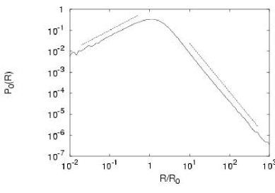
Figure 4:

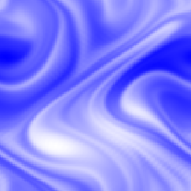
Figure 5:

Figure 6:

Figure 7:

References

- [1] P. G. De Gennes, Coil-stretch transition of dilute flexible polymer under ultra-high velocity gradients, J. Chem. Phys. 60:5030-5042 (1974).
- [2] T. T. Perkins, D. E. Smith, and S. Chu, Single Polymer Dynamics in an Elongational Flow, Science 276:2016-2021 (1997).
- [3] J. W. Hatfield and S. R. Quake, Dynamic Properties of an Extended Polymer in Solution, Phys. Rev. Lett. 82:3548-3551 (1999).
- [4] G. Falkovich, K. Gawȩdzki, and M. Vergassola, Particles and fields in fluid turbulence, Rev. Mod. Phys. 73:913-975 (2001).
- [5] E. Balkovsky, A. Fouxon, and V. Lebedev, Turbulent Dynamics of Polymer Solutions, Phys. Rev. Lett. 84:4765-4768 (2000).
- [6] E. Balkovsky, A. Fouxon, and V. Lebedev, Turbulence of polymer solutions, Phys. Rev. E 64:056301 (2001).
- [7] S. Gerashchenko, C. Chevallard, and V. Steinberg, Single polymer dynamics: coil-stretch transition in a random flow, to be published in Phys. Rev. Lett., arXiv:nlin.CD/0404045 (2004).
- [8] J. L. Lumley, On the solution of equations describing small scale deformation, Symp. Math. 9:315-334 (1972).
- [9] A. Gyr and H. W. Bewersdorff, Drag reduction of turbulent flows by additives (Kluwer Academic Publishers, Dordrecht, 1995).
- [10] G. K. Batchelor, Small-scale variation of convected quantities like temperature in turbulent fluid. Part 1. General discussion and the case of small conductivity, J. Fluid Mech. 5:113-133 (1959).
- [11] R. H. Kraichnan, Small-scale structure of a scalar field convected by turbulence, Phys. Fluids 11:945-963 (1968).
- [12] M. Chertkov, Polymer Stretching by Turbulence, Phys. Rev. Lett. 84:4761-4764 (2000).
- [13] J.-L. Thiffeault, Finite extension of polymers in turbulent flow, Phys. Lett. A 308:445-450 (2003).
- [14] E. Rouse, A Theory of the Linear Viscoelastic Properties of Dilute Solutions of Coiling Polymers, J. Chem. Phys. 21:1272-1280 (1953).
- [15] R. B. Bird, R. C. Armstrong, and O. Hassager, Dynamics of Polymeric Liquids, Fluid Mechanics, vol. I (Wiley, New York, 1977).
- [16] W. Kuhn, Über die Gestalt fadenförmiger Moleküle in Lösungen, Kolloid Z. 68:2-15 (1934).
- [17] R. B. Bird, O. Hassager, R. C. Armstrong, and C. F. Curtiss, Dynamics of Polymeric Liquids, Kinetic Theory, vol. II (Wiley, New York, 1977).
- [18] H. Risken, The Fokker-Planck Equation, Methods of Solution and Applications, in Springer Series in Synergetics, H. Haken ed. (Springer-Verlag, Berlin, Heidelberg, 1989).
- [19] J. L. Lumley, Drag reduction by additives, Annu. Rev. Fluid Mech. 1:367-384 (1969).
- [20] J. D. Schieber and H. C. Öttinger, The effect of bead inertia on the Rouse model, J. Chem. Phys. 89:6972-6981 (1988).
- [21] D. Vincenzi, unpublished (2004).
- [22] C. W. Gardiner, Handbook of Stochastic Methods for Physics, Chemistry, and the Natural Sciences, in Springer Series in Synergetics, H. Haken ed. (Springer-Verlag, Berlin, Heidelberg, 1985).
- [23] A. A. Monin and A. M. Yaglom, Statistical Fluid Mechanics, MIT Press, Boston, 1975.
- [24] A. Schenzle and H. Brand, Multiplicative stochastic processes in statistical physics, Phys. Lett. A 69:313-315 (1979).
- [25] A. Schenzle and H. Brand, Multiplicative stochastic processes in statistical physics, Phys. Rev. A 20:1628-1647 (1979).
- [26] R. Graham, Forward Hopf bifurcation with multiplicative gaussian white noise: exact Fokker-Planck solution, Phys. Lett. A 80:351-353 (1980).
- [27] R. Graham and A. Schenzle, Carleman imbedding of multiplicative stochastic processes, Phys. Rev. A 25:1731-1754 (1982).
- [28] K. Furutsu, On the statistical theory of electromagnetic waves in a fluctuating medium, J. Res. Nat. Bur. Standards D 67:303-323 (1963).
- [29] E. A. Novikov, Functionals and the random-force method in turbulence theory, Zh. Eksp. Teor. Fiz. 47:1919-1926 (1964) [Sov. Phys. JETP 20:1290-1294 (1965)].
- [30] U. Frisch, Turbulence: the legacy of A. N. Kolmogorov (Cambridge University Press, Cambridge, 1995).
- [31] R. H. Kraichnan, Convection of a passive scalar by a quasi-uniform random straining field, J. Fluid Mech. 64:737-762 (1974).
- [32] Y. Le Jan, Exposants de Lyapunov pour les mouvements browniens isotropes, C. R. Acad. Sci. Paris Sér. I 299:947-949 (1984).
- [33] Y. Le Jan, On Isotropic Brownian Motions, Z. Warscheinlichkeitstheorie verw. Gebiete 70:609-620 (1985).
- [34] D. T. Son, Turbulent decay of a passive scalar in the Batchelor limit: Exact results from a quantum-mechanical approach, Phys. Rev. E 59:R3811-R3814 (1999).
- [35] R. L. Stratonovich, Topics in the Theory of Random Noise (Gordon and Breach Science Publishers, Inc., New York, 1963).
- [36] I. S. Gradshteyn and I. M. Ryzhik, Table of Integrals, Series, and Products (Academic Press, New York, 1965).
- [37] G. Boffetta, A. Celani, and S. Musacchio, Two-dimensional Turbulence of Dilute Polymer Solutions, Phys. Rev. Lett. 91:034501 (2003).
- [38] B. Eckhardt, J. Kronjäger, and J. Schumacher, Stretching of polymers in a turbulent environment, Comput. Phys. Commun. 147:538-543 (2002).
- [39] R. H. Kraichnan and D. Montgomery, Two-dimensional turbulence, Rep. Prog. Phys., 43:547-619 (1980)
- [40] G. Boffetta, A. Celani, S. Musacchio, and M. Vergassola, Intermittency in two-dimensional Ekman-Navier-Stokes turbulence, Phys. Rev. E 66:026304 (2002).
- [41] E. Goursat, Léçons sur les séries hypergéométriques et sur quelques fonctions qui s’y rattachent, Vol. I (Hermann & C Editeurs, Paris, 1933).
- [42] E. T. Copson, An introduction to the theory of functions of a complex variable (Oxford University Press, Oxford, 1978).
- [43] L. Landau and E. Lifchitz, Quantum Mechanics, Nonrelativistic Theory (MIR Editions, Moscow, 1966).
- [44] A. Erdelyi et al., Tables of Integral Transforms (McGraw Hill, New York, 1954).