Emergence of chaotic attractor and anti-synchronization for two coupled monostable neurons

Abstract

The dynamics of two coupled piece-wise linear one-dimensional monostable maps is investigated. The single map is associated with Poincaré section of the FitzHugh-Nagumo neuron model. It is found that a diffusive coupling leads to the appearance of chaotic attractor. The attractor exists in an invariant region of phase space bounded by the manifolds of the saddle fixed point and the saddle periodic point. The oscillations from the chaotic attractor have a spike-burst shape with anti-phase synchronized spiking.

Spiking-bursting activity is a common feature of the temporal organization in many neural firing patterns john . Bursting activity means that clusters of spikes (of action potentials) occur more or less rhythmically and separated by phases of quiescence. Spiking-bursting dynamics can be regular or chaotic depending on the concentration of neuromodulators, currents and other control parameters. For example, many of the talamocortical neurons from central patterns generators generate chaotic spiking-bursting dynamics. In order to understand the emergence of chaotic oscillations in a neurones network, we use a two variables FitzHugh-Nagumo model of the membrane potential of an isolated neural cell. For appropriate values of the parameters, the system possesses a stable fixed point a focus surrounded by a separatrix such that for large enough perturbations, the system responds by an excitation pulse which also decays to the stable focus. Hence, introducing a section by a half-line, we obtain a one-dimensional piece-wise smooth map with one discontinuity point representing the excitation threshold. Then we consider a difference coupling between two such maps. In the linear approximation of the maps and for suitable values of the parameters, this two-dimensional system is locally hyperbolic having discontinuity lines and a strange attractor . The interesting fact is that these lines define regions in the phase space corresponding to the thresholds of excitability of each one of these neurones, or none of them. The symbolic dynamics represents then the bursting activity of the neurones. It is then possible to apply the approximation tools of statistical analysis of time series generated by the system, namely through Perron-Frobenius Operator, in order to study and interpret some important features of neural networks, like synchronization and time correlations.

I Introduction

Many neural systems composed of a number of interacting neurons exhibit self-sustained oscillatory behavior leading to the formation of various space-time patterns. Such patterns are believed to play a key role in signal and information processing functions of the brain kan ; mur ; sco . One of the fundamental problems is the understanding of possible dynamic mechanisms of such patterns to appear and to evolve in time and space man ; loe ; sher ; wang1 ; rul ; vries ; kop ; pinto . There are two basic phenomena of emergence of oscillations (regular or chaotic) in neuron assemblies. The first one is obvious and deals with the presence of local intra-cellular oscillations. Being coupled such units are capable of various oscillatory patterns, clustering and synchronization. The second one, found in recent theoretical and experimental studies, concerns the possibility of oscillations in assemblies of non-oscillatory cells man ; loe ; sher . The oscillations may also appear in coupled non-identical cells for sufficiently strong coupling. The assembly is characterized by an oscillatory “average” cell dynamics which makes the non-oscillatory cells oscillating. Another studies have reported that coupling even identical excitable cells can modify the dynamics to form oscillatory attractors co-existing with a stable fixed point sher . Such attractors are characterized by anti-phase spiking. The effects of electrical coupling between neural cells also include the appearance of bursting in two coupled pacemaker cells, modification of burst period in coupled bursters, synchronization and chaos wang1 ; rul ; vries ; kop ; pinto ; rul1 .

A model approach, in order to display the dynamical origin of neural oscillations, is to use a simplified behavior-based description of the system. For this purposes nonlinear maps could be helpful as they can provide an appropriate qualitative description of complex dynamic processes including chaotic behavior in lower dimensional systems rul ; vries ; courb . In this paper we study the system of two coupled piece-wise linear one-dimensional maps. The single map is derived from the dynamics of an isolated neural cell modelled by the FitzHugh-Nagumo excitable system sco ; izh ; kaz . The FitzHugh-Nagumo neuron model can be derived from Hodgkin-Huxley conductance-based model, for some parameter values, when we take into account the difference of kinetics between the potential dependent gating variables kan . The first variable describes the evolution of neuron membrane potential, the second mimics the dynamics of outward ionic currents. Then, the model can describe the salient features of neuron dynamics including the action potential generation, excitability and excitation threshold.The map has one globally stable fixed point and a discontinuity corresponding to the excitation threshold of the cell. We shall show how linear diffusive coupling between the two maps leads to the appearance of chaotic oscillations with anti-phase spiking. A number of studies of coupled chaotic maps have shown that anti-phase chaotic oscillations may appear when the synchronization manifold looses transverse stability and the system evolves to the off-diagonal attractors car ; gle ; ash ; ash1 ; lai ; courb .

The paper is organized as follows. In Sect. II we show how the dynamics of excitable FitzHugh-Nagumo model can be described by a piece-wise continuous point map and introduce two-dimensional map modeling a pair of coupled cells. In Sect. III we analyze the dynamics of the map. We numerically show the emergence of strange attractor in an invariant domain defined by invariant manifolds of saddle fixed point and saddle periodic orbit. Sect. IV describes the statistical characteristics of the attractor set and the emergent chaotic oscillations with anti-phase spiking. Section V contains a brief discussion of the results.

II Point map description of the excitable dynamics

To replicate the excitable dynamics of an isolated neural cell one can use the FitzHugh-Nagumo-like model. It can be taken in the following form

$$\begin{array}[]{l}\vspace{0.05 in}\dot{u}=u-u^{3}/3-v,\\ \vspace{0.05 in}\dot{v}=\epsilon(k(u)-v-I),\\ \end{array}$$ (1)

The $u$-variable describes the evolution of the membrane potential of the neuron, $v$ describes the dynamics of the outward ionic currents (the recovery variable) sco .The function $k$ is taken piece-wise linear, $k(u)=k_{1}u$, if $u<0$, and $k(u)=k_{2}u$, if $u\geq 0$. The parameters $k_{1}$ and $k_{2}$ control the shape and the location of the $v$-nullcline, hence the dynamics of the recovery term. The parameter $\epsilon$ defines the time scale of excitation pulse and the parameter $I$ is a constant stimulus. The excitable behavior of Eqs. (1) is illustrated in Fig. 1. Appropriate values of the parameters provide the existence of three fixed points $O_{1}(u^{(1)},v^{(1)})$, $O_{2}(u^{(2)},v^{(2)})$ and $O_{3}(u^{(3)},v^{(3)})$. The points $O_{1}$ and $O_{3}$ are stable and unstable foci, respectively, the point $O_{2}$ is a saddle with the incoming separatrix defining the excitation threshold. Then, if a perturbation of the rest state, $O_{1}$, is large enough, i.e. lies beyond the separatrix, the system responds with an excitation pulse, otherwise it decays to the stable rest point $O_{1}$ (Fig. 1).

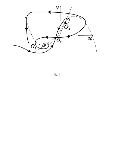
Figure 1: Qualitative picture of the phase plane of Eqs. (1). $S$ illustrates the transversal half-line.

In order to describe the dynamics of the unit (1) by a point map, we introduce the transversal half-line $L:\{v=v^{(1)},u>u^{(1)}\}$ (Fig. 1). It is found that the return map of the flow given by Eqs. (1) at the section $L$ defines a map, $\Phi:L\rightarrow L$, for all points excluding the one, $L_{0}$, corresponding to the intersection of the incoming saddle separatrix with the half-line $L$. This point never returns to the cross-section. Consequently, we also must exclude all the pre-images of the point $L_{0}$, $L_{k}=(\Phi^{-1})^{m}L_{0}$, $m=1,2,\ldots,\infty$ . Then, the Poincaré map $\Phi$ can be written as

$$x(n+1)=\Phi(x(n)),$$ (2)

$$n=1,2,\ldots,\infty,$$

with $x(n)$ accounting for $(u-u^{(1)})$-coordinates of the points at the Poincare section. The map is invertible and defined in the interval $[0,\infty)$ excluding the points $L_{k}$ . The shape of the curve $\Phi(x)$ calculated numerically is shown in Fig. 2. It is given by a piece-wise continuous curve with one stable fixed point. Then, the dynamics of the map is trivial. All its trajectories represent sequences of points monotonically approaching to the fixed point. The discontinuity point plays the role of the excitation threshold, i.e. the neuron exhibits spiking if the map evolves above this point. Note, that such map obtained from (1) gives an “average” description of the cell dynamics.

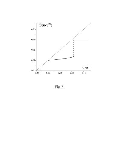
Figure 2: The curve $\Phi(x)$ obtained from Eqs. (1) at the section half-line $L$. Parameter values: $\epsilon=0.5,k_{1}=0.5,k_{2}=2,I=0.221$.

Let us approximate the piece-wise continuous curve $\Phi(x)$ by a piece-wise linear function and define the map for all points $(-\infty,\infty)$ excluding the points $L_{k}$. Then, for two cells we introduce difference coupling term (electrical coupling) and consider the following two-dimensional map $f$: $R^{2}\longrightarrow\ R^{2}$

$$\begin{array}[]{l}\vspace{0.05 in}x_{1}(n+1)=F(x_{1}(n))+d(x_{2}(n)-x_{1}(n)),\\ \vspace{0.05 in}x_{2}(n+1)=F(x_{2}(n))+d(x_{1}(n)-x_{2}(n)),\end{array}$$ (3)

where the variables $x_{1,2}$ refer to the dynamics of the two cells, $d$ is the coupling coefficient, the function $F(x)$ is taken in the form

$$F(x)=\left\{\begin{array}[]{l}\alpha x,\;\mbox{if}\;x\leq a;\\ \alpha x+\alpha(b-a)\;\mbox{if}\;x>a,\end{array}\right.$$ (4)

$0<\alpha<1$.

III Dynamics of the map

A. General properties of map

Since $F(x)$ is given by the piece-wise linear function, then the differential $Df$ of the map $f$ is a constant matrix, with eigenvalues

$$\mu_{1}=\alpha-2d,\;\mu_{2}=\alpha$$ (5)

.

Hence, Lyapunov exponents are defined by $\lambda_{i}=\ln|\mu_{i}|,i=1,2$, for a arbitrary trajectory of the map, except zero Lebesgue measure set of initial conditions.

Let us consider the system (3) in the parameter region

$D=\{\alpha,d,a:\;0<\alpha<a/b,\;\frac{1+\alpha}{2}<d<1,\;a>0\}$

For convenience, we shall fixed $a=1$. This region $D$ is chosen in order to have Lyapunov exponents $\lambda_{1}>0,\;\lambda_{2}<0$, hence any trajectory, $\{f^{i}x_{0},\;x_{0}\notin B\}$, where $B$ is a set of discontinuous points of the map $f$, is heavily dependent on initial conditions, and to have the modulus of Jacobian of the map $f$ less than one, in $D$. All these features allow us to speak of chaotic behavior.

We shall study the trajectories of the map $f$ missing the discontinuity set $B=\bigcup\limits_{i=0}^{\infty}f^{-i}\gamma$, where

$$\gamma=\{x_{1},x_{2}:\{x_{1}=a\}\bigcup\{x_{2}=a\}\}$$ (6)

For convenience, let us change variables, according to the eigenvectors of $Df$

$$y_{1}(n)=x_{2}(n)-x_{1}(n),\;y_{2}(n)=x_{2}(n)+x_{1}(n)$$ (7)

Then, the discontinuity lines become

$$\begin{array}[]{l}\Gamma_{1}=\{y_{1},y_{2}:\;y_{2}-y_{1}=2a\}\\ \Gamma_{2}=\{y_{1},y_{2}:\;y_{2}+y_{1}=2a\}\end{array}$$

The lines $\Gamma_{1}$ and $\Gamma_{2}$ divide the phase plane $(y_{1},y_{2})$ of the map $f$ into four regions

$$\begin{array}[]{l}G_{1}=\{y_{1},y_{2}:\;y_{2}+y_{1}<2a,\;y_{2}-y_{1}<2a\}\\ G_{2}=\{y_{1},y_{2}:\;y_{2}+y_{1}>2a,\;y_{2}-y_{1}<2a\}\\ G_{3}=\{y_{1},y_{2}:\;y_{2}+y_{1}<2a,\;y_{2}-y_{1}>2a\}\\ G_{4}=\{y_{1},y_{2}:\;y_{2}+y_{1}>2a,\;y_{2}-y_{1}>2a\}\par\end{array}$$

In each region $G_{i}$ the map $f$ is continuous and has the form

$$\left\{\begin{array}[]{l}y_{1}(n+1)=\mu_{1}y_{1}(n)+b_{1}\\ y_{2}(n+1)=\mu_{2}y_{2}(n)+b_{2},\end{array}\right.$$ (8)

with

$$b_{1}=\left\{\begin{array}[]{l}0,\;if\;(y_{1},y_{2})\in G_{1},G_{4}\\ \alpha(b-a),\;if\;(y_{1},y_{2})\in G_{2}\\ -\alpha(b-a),\;if\;(y_{1},y_{2})\in G_{3}\end{array}\right.$$

$$b_{2}=\left\{\begin{array}[]{l}0,\;if\;(y_{1},y_{2})\in G_{1}\\ \alpha(b-a),\;if\;(y_{1},y_{2})\in G_{2},G_{3}\\ 2\alpha(b-a),\;if\;(y_{1},y_{2})\in G_{4}\end{array}\right.$$

The map $f$ has one hyperbolic fixed point, $O(0,0)$. In region $G_{1}$ its invariant curves coincide with the coordinate axes. Analyzing map $f$ in the regions $G_{2}$, $G_{4}$ we find that it has a hyperbolic periodic orbit, $Q$, of period two with coordinates

$$y_{1}=\frac{\alpha(b-a)}{2d-\alpha-1}\equiv y_{1}(Q),\;\;\;\;\;y_{2}=\frac{\alpha(b-a)}{1-\alpha}\equiv y_{2}(Q),$$ (9)

if the parameters satisfy the inequality

$$d<d_{p}\;\;\;\mbox{with}\;\;\;d_{p}\equiv\frac{2a-\alpha^{2}(a+b)}{2[2a-\alpha(a+b)]}.$$ (10)

Stable and unstable invariant manifolds of the orbit $Q$ are

$$W^{s}(Q)=\left\{y_{1},y_{2}:\;\begin{array}[]{l}y_{1}=y_{1}(Q),\;\;\;\;if\;(y_{1},y_{2})\in G_{2}\\ y_{1}=-y_{1}(Q),\;if\;(y_{1},y_{2})\in G_{3}\\ \end{array}\right.$$

$$\;\;W^{u}(Q)=\{\;y_{1},y_{2}:\;\;y=y_{2}(Q),\;if\;(y_{1},y_{2})\in G_{2},G_{2}^{-}\}$$

It follows from (9) that

$$\lim_{d\to\frac{1+\alpha}{2}+0}y_{1}(Q)=+\infty.$$

Then periodic orbit $Q$ appears from infinity in the phase plane $(y_{1},y_{2})$ for the parameters belonging to the curve

$$N_{-1}=\left\{\alpha,d:\;\;d=\frac{1+\alpha}{2},\;\;0<\alpha<\frac{a}{b}\right\}$$

in the parameter plane $(\alpha,d)$. Note, that on this curve one of the multiplier hits the bifurcation value, $\mu_{1}=-1$. Then fixed point $O$ changes its stability becoming of saddle type in $D$.

B. Invariant region and chaotic attractor of the map $f$

Let us consider the location of invariant curves of the points $O$ and periodic orbit $Q$ in the phase plane with respect to the lines $\Gamma_{1},\;\Gamma_{2}$. The unstable invariant curve (the separatix) $W^{u}_{1}(Q)$ intersects the line $\Gamma_{2}$ at point $K$ with coordinates

$$y_{1}=\frac{2a-\alpha(b+a)}{1-\alpha},\;\;\;\;\;y_{2}=y_{2}(Q),$$ (11)

and invariant curve $W^{u}_{1}(O)$ at the point $M$ with coordinates

$$y_{1}=2a,\;\;\;\;\;y_{2}=0,$$ (12)

Figure 3 illustrates the location of the invariant curves of fixed point $O$ and orbit $Q$ in the phase plane $(y_{1},y_{2})$.

Let us introduce region $\Pi$ in the phase plane defined by

$$\Pi=\left\{y_{1},y_{2}:\;\;-y_{1}(Q)<y_{1}<y_{1}(Q),\;\;\;0<y<y_{2}(Q)\right\}$$

Let us find the conditions for region $\Pi$ to be an invariant region of map $f$. Since the system (8) is symmetric with respect to $y_{2}$-axis it is sufficient to consider only $y_{1}\geq 0$ region. Assuming ${(y_{1}(0),y_{2}(0))\in G_{1}^{+}}$, where ${G_{1}^{+}=\{\Pi\setminus B\}\bigcap G_{1}\bigcap\{y_{1}\geq 0\}}$, let us obtain the conditions on the parameter values for which ${(y_{1}(1),y_{2}(1))\in\Pi}$. In region $G_{1}^{+}$ we find that

$$\left\{\;\begin{array}[]{l}y_{1}(1)=-(2d-\alpha)y_{1}(0)\\ y_{2}(1)=\alpha y_{2}(0)\end{array}\right.$$ (13)

It follows from (13) that ${(y_{1}(1),y_{2}(1))\in\Pi}$ if the following inequalities

$$-\frac{y_{1}(Q)}{2d-\alpha}<y_{1}(0)<\frac{y_{1}(Q)}{2d-\alpha}\;\;\;\;\;\;\;\;y_{2}(0)<\frac{y_{2}(Q)}{\alpha}$$ (14)

are satisfied. Using the symmetry of $f$ with respect to $y_{1}$, we can restrict the above condition to the right part of $\Pi$, and since

$$\begin{split}\max_{{(y_{1}(0),y_{2}(0))\in G_{1}^{+}}}y_{1}(0)&<y_{1}(M),\\ \max_{{(y_{1}(0),y_{2}(0))\in G_{1}^{+}}}y_{2}(0)&<y_{2}(Q)\end{split}$$ (15)

the inequalities (14) are satisfied if

$$\frac{y_{1}(Q)}{2d-\alpha}>y_{1}(M),\;\;\;\;\;\;\;\;\frac{y_{2}(Q)}{\alpha}>y_{2}(Q)$$ (16)

The first inequalities in (16)impose the following condition on $d$:

$$d<d_{h}\;\;\mbox{with}\;\;d_{h}\equiv\frac{1+2\alpha+\sqrt{1+\frac{2\alpha(b-a)}{a}}}{4}$$ (17)

Thus, under the condition (17) $f(G_{1}^{+})\subseteq\Pi$. Similarly we find that the image of ${G_{2}^{+}=\{\Pi\setminus B\}\bigcap G_{2}\bigcap\;\{y_{1}>0\}}$ by $f$ is also included in $\Pi$, for the parameter in $D$.

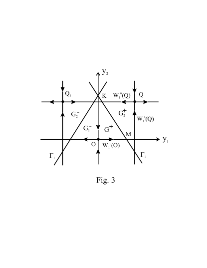
Figure 3: Mutual location of invariant manifolds of the fixed point $O$ and periodic orbit $Q$, and discontinuity lines $\Gamma_{1,2}$ on the phase plane of map $f$.

Finally, $\Pi$ is invariant region of map $f$ in the parameter region

$$D_{inv}=D\bigcap\{d<d_{p}\}\bigcap\{d<d_{h}\}$$

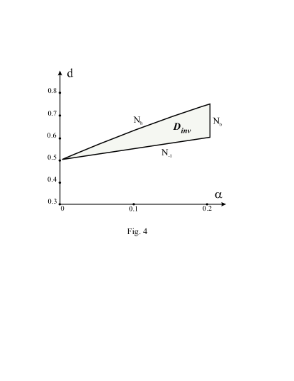
Figure 4: Parameter region $D_{inv}$ on the parameter plane $(\alpha,d)$.

Figure $4$ shows region $D_{inv}$ in the parameter plane $(\alpha,d)$. In this plane the boundary of $D_{inv}$ consists of three components:

$$\begin{array}[]{l}N_{-1}=\left\{\alpha,d:\;d=\frac{1+\alpha}{2},\;0<\alpha<\frac{a}{b}\right\}\\ N_{b}\;\;=\left\{\alpha,d:\;\alpha=\frac{a}{b},\;\frac{a+b}{2b}<d<d_{h}\right\}\\ N_{h}\;\;=\left\{\alpha,d:\;d=d_{h},\;0<\alpha<\frac{a}{b}\right\}.\end{array}$$

The line $N_{-1}$ corresponds to the appearance of periodic orbit $Q$ and changing stability of the fixed point $O$. The line $N_{b}$ is the boundary of the monostability of the uncoupled, $d=0$, maps (3). The points of the curve $N_{h}$ corresponds to the ”tangency” of the separatricies $W_{1}^{u}(O)$ and $W_{1}^{s}(Q)$, and for these parameter values $f(M)\in W_{1}^{s}(Q^{-})$.

Therefore, if the parameter values of system (8) belongs to region $D_{inv}$, then invariant (absorbing) region $\Pi$ and $\overline{f(\Pi\setminus B)}\subset\Pi$ exists in the phase plane. Consequently, $\Pi$ contains strange (chaotic) attractor $A$ of the map $f$. Figure 5 illustrates possible structure of the attractor $A$ in the phase plane.

Figure 5: Chaotic attractor $A$ on the phase plane $(y_{1},y_{2})$. Parameter values: $b=4.95,\alpha=0.2,d=0.74$.

To characterize the complexity of the chaotic attractor $A$ we calculated numerically its fractal dimension $d_{f}(A)$. It appears that, indeed, $d_{f}(A)$ takes non-integer values greater than $1$ (Fig. 6). Note that the box dimension of the set increases with the increase of coupling coefficient $d$. Corresponding estimate of the dimension $d_{f}$ using Lyapunov exponents $\Lambda_{i}$ is shown by dashed curve.

Figure 6: Fractal dimension $d_{f}(A)$ of the chaotic attractor $A$ calculated by box counting method versus coupling coefficient $d$. Parameter values: $b=4.95,\alpha=0.2$.

Figure 7: (a) Chaotic oscillations of the map (2). $x_{1,2}(n)$ are shown by solid and dashed curves, respectively. (b) Spike-burst behavior of binary variables $z_{1,2}(n)$. Parameter values: $b=4.95,\alpha=0.2,d=0.74$.

C. Chaotic oscillations and attractor.

Figure 7 (a) illustrates time evolution of the variables $x_{1}(n),x_{2}(n)$ corresponding to chaotic attractor $A$. Let us characterize the oscillations in terms of original model (1) describing neuron excitability. Note that the neuron excitation threshold accounted by saddle separatrix (Fig. 1) corresponds to the discontinuity lines $\Gamma_{1},\Gamma_{2}$ in the map description. Thus, if a map trajectory jumps above these lines then we can refer this event as a neuron spike, if it evolves below $\Gamma_{1},\Gamma_{2}$, the neuron is not excited . In such a way the map oscillations can be described with binary variables $z_{i}$:

$$z_{i}(n)=\left\{\begin{array}[]{ll}0,\mbox{if}&x_{i}(n)<a;\\ 1,\mbox{if}&x_{i}(n)>a.\end{array}\right.$$

The evolution of $z_{i}$-variables is shown in Fig. 7 (b). It appears that map oscillation represent sequence of bursts containing anti-phase spiking. Note that characteristic time scales of oscillations (burst duration and inter-burst period) depend coupling $d$. For smaller $d$ one can find longer lasting subthreshold period and shorter burst period. Then, the map describes a kind of chaotic spike-burst behavior typical for many neural systems.

IV Stationary probability distribution on the chaotic attractor

The global behavior of the chaotic dynamics is described by the probability of finding the trajectory in any given region of the attractor. It can be visualized by a distribution of a cloud of points, each moving under the deterministic mapping. A stationary distribution may be reached by the system after long term evolution. To obtain this distribution, we start from a histogram of clouds of points in each small “box” of the phase space. These points are mapped by $f$ and a new cloud is thus obtained. Thus to the initial probability density $\rho_{0}$ correspond a new density $\rho_{1}$. The operator which maps $\rho_{0}\longrightarrow\rho_{1}$ is called the Perron-Frobenius operator: $\rho_{1}=P\rho_{0}$ defined by:

$$\int_{A}P\rho_{0}(y_{1},y_{2})dy_{1}dy_{2}=\int_{f^{-}1(A)}\rho_{0}(y_{1},y_{2})dy_{1}dy_{2}$$ (18)

for any region $A$ of the phase space. The stationary density $\rho$ is an eigenfunction of $P$ corresponding to the eigenvalue $1$. The existence and uniqueness of the stationary distribution has been the object of many works boya ; wang1 . It is nevertheless difficult to obtain analytical exact expression of $\rho(y_{1},y_{2})$, apart from the restricted case of Markov maps. We shall use an approximating algorithm inspired from the method of Ding and Zhou ding .

The phase space of the coupled system is divided into $n\times m$ identical rectangles $\Delta_{i}$. We consider an initial probability density $\rho_{o}(y_{1},y_{2})$ that is constant on each $\Delta_{i}$:

$$\rho_{0}(Y)=\sum_{i=1}^{n\times m}\frac{a_{i}(0)}{m(\Delta_{i})}\chi_{\Delta_{i}}(Y)$$ (19)

where $Y=(y_{1},y_{2})$, $m(\Delta_{i})$ is the Lebesgue measure of $\Delta_{i}$ and $a_{i}(0)$ is the probability of finding a phase point in $\Delta_{i},\;\chi_{\Delta_{i}}$ is the characteristic function of $\Delta_{i}$:

$$\chi_{\Delta_{i}}(Y)=\left\{\begin{array}[]{l}1\;\;\;\;if\;\;\;Y\in\Delta_{i}\\ 0\;\;\;\;if\;\;\;Y\notin\Delta_{i}\\ \end{array}\right.$$

It is clear that $\rho_{1}$ has no reason to be of the “Coarse-grained” form (19). Smoothing this density by integrating it on each $\Delta_{j}$ we obtain by using the definition (18):

$$\begin{array}[]{rcl}a_{j}(1)&=&\int_{\Delta_{j}}P\rho_{0}(Y)dY\\ &=&\int_{f^{-1}(\Delta_{j})}\rho_{0}(Y)dY\\ &=&\int_{f^{-1}(\Delta_{j})}[\sum_{i}\frac{a_{i}(0)}{m(\Delta_{i})}\chi_{\Delta_{i}}(Y)]dY\\ &=&\sum_{i}\frac{a_{i}(0)}{m(\Delta_{i})}\int_{\Delta_{j}}\chi_{\Delta_{i}}(Y)]dY\\ &=&\sum_{i}a_{i}(0)\frac{m(f^{-1}(\Delta_{j})\bigcap\Delta_{i})}{m(\Delta_{i})}\\ \end{array}$$ (20)

Thus, the transition probability from $\Delta_{i}$ to $\Delta_{j}$ is given by the stochastic matrix:

$$p_{i,j}=m(f^{-1}(\Delta_{j})/\Delta_{i})\equiv\frac{m(f^{-1}(\Delta_{j})\bigcap\Delta_{i})}{m(\Delta_{i}}))$$ (21)

The matrix $p=(p_{i,j})$ is an approximate value of the Perron-Frobenius operator $P$. It can be proved that $p$ converges to $P$ as $|\Delta_{i}|\longrightarrow 0$ ding . Eq. (20) can be written under the matrix form:

$$a(t+1)=a(t)p,\ t=0,\ldots$$ (22)

where $a(t)$ is the row vector $(a_{1}(t),\ldots,a_{N}(t))$ with $N=n\times m$. Thus, an approximate stationary probability is the row eigenvector $\upsilon=(\upsilon_{1}(n),\ldots,\upsilon_{N}(n))$ such that:

$$\upsilon=\upsilon\cdot p,$$ (23)

We first calculate the matrix elements of $p$ and then we compute the eigenvector $v$. To calculate $p_{i,j}$ we use (21). In each rectangle $\Delta_{i}$ we put $k\times l$ points uniformly distributes - then we compute the number of point $(Y\in\Delta_{i})$ such that $f(Y)\in\Delta_{j}$, and we divide this number by the number of points in $\Delta_{i}$. This provides $p_{i,j}$.

We used this method to approximate the stationary distribution for $\alpha=0,2$ and $d=0,75$ (Fig. 8) showing a density distributed over some region, which is to be compared with the Fig. 5 where we have used only one trajectory. It is to be noted that the last figure shows the attractor generated by one trajectory whereas Fig.8 shows the approximate density of the attractor.

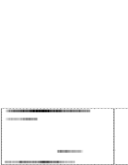
Figure 8: Approximative stationary distribution of the map $f$.Parameter values: $b=4.95,\alpha=0.2,d=0.74$.

V Synchronization.

The above method allows to obtain the statistical distribution of synchronized spikes. Recall that the variable $x_{1}$ is spiking if and only if $Y\in G_{2}^{-}$ and $x_{2}$ is spiking if and only if $Y\in G_{2}^{+}$, and no one is spiking if $Y\in G_{1}^{+}\cup G_{1}^{-}$ which we denote $G_{1}$. Recall also that the region $G_{4}$ corresponds to $x_{1}$ and $x_{2}$ are simultaneously spiking, which lies outside the invariant region. Moreover, because $G_{1},\ G_{2}^{\pm}$ are disjoint, $x_{1}$ and $x_{2}$ cannot be simultaneously spiking . Thus we shall consider a partition of the invariant domain $\Pi$ corresponding to one of the three possible states of spiking $S(Y)$:

$$\begin{array}[]{rcl}S(Y)=x_{1s}&\;if&Y\in G_{2}^{-}\\ S(Y)=x_{2s}&\;if&Y\in G_{2}^{+}\\ S(Y)=0&\;if&Y\in G_{1},\\ \end{array}$$

where $x_{is}$ means that the only spiking variable is $x_{i}$; and $0$ means that no one is spiking. This partition induces symbolic dynamics, that we shall study. We calculate the stochastic matrix $\pi_{i,j}$ from any one of these states to any other, where $i,j$ are the states $x_{1s},x_{2s},0$, for two values of the coupling parameter $d=0.65,\ 0.7$ (see Fig. 9).

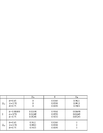
Figure 9: The $3*3$ stochastic matrices of transition probabilities for three values of the coupling d.

This table shows that we have only the following probable transitions in one step:

$$x_{2s}\longrightarrow x_{1s}\longrightarrow x_{2s}$$

and $0\longleftrightarrow 0$.

Less probable transitions are:

$$x_{1s}\longrightarrow 0,\;\;\;x_{2s}\longrightarrow 0$$

$$0\begin{array}[]{ll}&x_{1s}\\ \nearrow&\\ \searrow&\\ &x_{2s}\\ \end{array}$$

but these transition probabilities depend monotonically on the coupling $d$. Thus the transitions $x_{1s}\longrightarrow x_{2s}$ and $x_{2s}\longrightarrow x_{1s}$ (i.e. successive spikes) decreases slightly with coupling. So, strengthening the coupling in this range decreases the bursting probability.

We can understand these occurrences in considering the intersections of the image of each region by $f$ with these same regions (see Fig. 10). The most probable transition $x_{ls}\longrightarrow x_{ks},\ \{k,l\}\in\{1,2\}^{2}$ and $0\longrightarrow 0$ correspond respectively to $f(G_{2}^{\pm})\bigcap G_{2}^{\mp}$ and $f(G_{1})\bigcap G_{1}$. The less probable transitions $x_{ls}\longrightarrow 0$ and $0\longrightarrow x_{ls}$ correspond respectively to $f(G_{2}\pm)\bigcap G_{1}$ and $f(G_{1})\bigcap G_{2}^{\pm}$. The positive Lebesgue measure of these intersected regions give the transition probabilities of each of these occurrences. Some of the transition probabilities given by the calculation of the Lebesgue measures of the intersected regions are shown in Fig. 11, with their dependance over the coupling constant $d$, which can be compared to those obtained numerically in the table Fig. 9. All the calculations are made in appendix A, where we also show that ,when the parameters are in $D_{inv}$,a neuron can not fire twice, i.e. $G_{2}^{\pm}\bigcap f(G_{2}^{\pm})=\emptyset$.

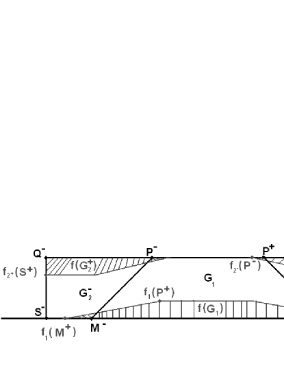
Figure 10: Image by $f$ of the partitions of the invariant region $\Pi$.

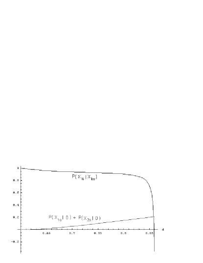
Figure 11: Probability transition from a spike to another, and from rest to spike, versus coupling constant $d$; $b=4.95,\alpha=0.2$.

We can now check the memory effects in studying the conditional probability of a state given the past. If we denote by $S_{0},S_{-1},S_{-2}\ldots$ the values of the variable $S$ at time, $0,\;-1,\;-2$ etc, we like to know if conditional probability $Prob(S_{0}|S_{-2},S_{-1})$ is equal to $Prob(S_{0}\;|\;S_{-1})$ or not. In the first case there is no memory of the process. In order to compute the above conditional probability we have to find $Prob(S_{0}=i_{0}\;|\;S_{-2}=i_{-2},S_{-1}=i_{-1})$ which implies $(3)^{3}=27$ calculations. But, neglecting rare events like $S_{-2}=0,S_{-1}=x_{2s}$ having $0,0422$ probability for $d=0,75$, we have only $4$ significant transitions.

$$\begin{array}[]{l}Prob(S_{0}=x_{2s}\;|\;S_{-2}=x_{2s},\;S_{-1}=x_{1s})=P_{1}\\ Prob(S_{0}=x_{1s}\;|\;S_{-2}=x_{1s},\;S_{-1}=x_{2s})=P_{2}\\ Prob(S_{0}=0\;|\;S_{-2}=x_{2s},\;S_{-1}=x_{1s})=P_{3}\\ Prob(S_{0}=0\;|\;S_{-2}=x_{1s},\;S_{-1}=x_{2s})=P_{4}\end{array}$$

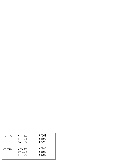
Figure 12: The conditional probabilities of spiking and non-spiking after two successive spikes respectively.

The first one is the probability of having $x_{2s}$ if it is preceded by a sequence of $x_{2s}$ and $x_{1s}$ and for the others the definition is the same. Thus we obtain the following table (Fig.12). The fact that the probability $P_{1}=0,879$ is not equal to $Prob(S_{0}=x_{2s}\;|\;S_{-1}=x_{1s})=0,9303$ means that the system has acquired a memory, the chain is not a Markov chain. The memory of a chain is given by the smallest positive integer $m_{o}$ such that:

$$Prob(S_{0}\;|\;S_{-m},\;S_{-m+1},\ldots,S_{-1})=Prob(S_{0}\;|\;S_{-m_{0},\ldots,S_{-1}})$$

for any $m\geq m_{o}$, and any value of $(S_{0},\ldots S_{-m})$.

It is also remarkable that the probability of having $0$ if it is preceded by the sequence $(x_{2s},\;x_{1s})$ is $0,1209$ the double of the probability of having $0$ preceded by $x_{1s}$ simply $0,0696$. This explain the frequent appearance of sequence of spikes. How could we estimate the memory of the process depends on the full calculation of all conditional probabilities for all past.

Another very interesting aspect is the dependence of this memory on the coupling coefficient as shown in Fig. 13. It is clear that the memory effects increase with coupling (the distance between the two curves increases with coupling).

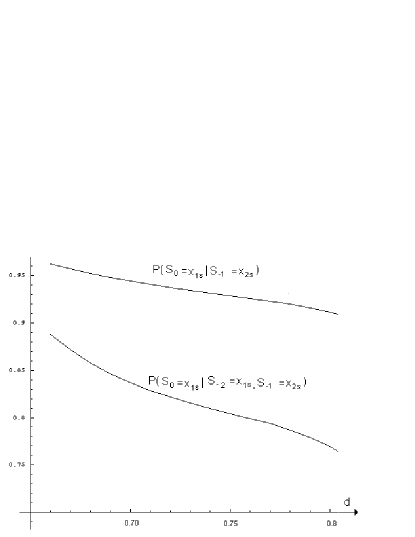
Figure 13: The effect of coupling on the memory effect. Parameter values: $b=4.95,\alpha=0.2$.

VI Conclusion

We have investigated chaotic dynamics of two coupled maps each formally derived from FitzHugh-Nagumo model of neuron excitability. Being uncoupled such maps are trivial with only one stable fixed point corresponding to neuron rest state. The excitation threshold is given by the discontinuity point. We have introduced the formal definition of spike if the map evolves above this threshold. The linear “diffusive” coupling term introduced for the maps can be treated as a kind of electrical inter-neuron coupling that mimics an “integral” coupling current between the two cells.

We have shown that increasing the coupling coefficient above certain threshold leads to the appearance of chaotic attractor. The attractor appears in the invariant region of the phase space confined by the invariant manifolds of saddle periodic orbit. This region attracts trajectories from outside and does not contain any stable trajectory inside. The oscillations emerging with such an attractor have a spike-burst shape with synchronous bursts with anti-phase spiking. Using probabilistic description we have found the probabilities to find a spike in different conditions. It has been also found that the system acquires a memory (in contrast with Markov’s processes).

Acknoledgments

This research has been supported by Russian Foundation for Basic Research (grants 03-02-17135) and by grant of President of Russian Federation (MK 4586.2004.2). V.B.K. acknowledges Russian Science Support Foundation for financial support. V.I.N. acknowledges the financial support from University Paris VII.

Appendix A Image of the invariant region after one iteration.

In order to understand the oscillatory behavior it is interesting to look at the image of the invariant region after one iteration (see Fig. 10). First of all, we have to determine the images of the regions of the invariant region, defined by the discontinuities, namely $G_{1}$, $G_{2}^{+}$ and $G_{2}^{-}$(e.q. to $G_{2}^{-}$).

$G_{1}$ is a polygon having for vertices $P^{+}$, $P^{-}$, $M^{+}$ and $M^{-}$; $G_{2}^{+}$, $Q^{-}$, $P^{-}$, $S^{-}$ and $M^{-}$; and $G_{2}^{-}$ , $P^{+}$, $Q^{+}$, $S^{+}$ and $M^{-}$ (when $M^{+}<S^{+}$ or equivalent, which is always satisfied for $d<d_{h}$). Let us compute the images of all these vertex, according to the definition of $f$ in each region. We have to keep in mind that some of these points belong to the lines of discontinuity; in this case, the computation is taken in the sense of a limit starting from the interior of each region.

First, we compute the image of $G_{1}$ obtained by the image of its vertices:

$$\begin{array}[]{l}f_{1}(M^{+})=\{2a(\alpha-2d),0\},\\ f_{1}(M^{-})=\{-2a(\alpha-2d),0\},\\ f_{1}(P^{+})=\{{(\alpha(b+a)-2a)(\alpha-2d)\over\alpha-1},{\alpha^{2}(a-b)\over\alpha-1}\},\\ f_{1}(P^{-})=\{-{(\alpha(b+a)-2a)(\alpha-2d)\over\alpha-1},{\alpha^{2}(a-b)\over\alpha-1}\},\end{array}$$ (24)

we shall show that $(f(G_{1})\bigcap G_{2}^{+})\bigcup(f(G_{1})\bigcap G_{2}^{-})\neq\emptyset$, which means that a neuron at rest can fire. That is to say

$$\begin{array}[]{l}y_{1}(f_{1}(M^{-}))>y_{1}(M^{+}),\\ -2a(\alpha-2d)>2a\end{array}$$ (25)

However, the last inequality is always true when we are in $D_{inv}$.

Next, we compute the image of $G_{2}^{+}$:

$$\begin{array}[]{l}f_{2}(M^{+})=\{\alpha(-a+b)+2a(\alpha-2d),\alpha(-a+b)\},\\ f_{2}(P^{+})=\{{\alpha b(-2\alpha+1+2d)+a(\alpha+2d(\alpha-2))\over 1-\alpha},{\alpha(b-a)\over 1-\alpha}\},\\ f_{2}(Q^{+})=\{{\alpha(b-a)\over\alpha+1-2d},{\alpha(b-a)\over 1-\alpha}\},\\ f_{2}(S^{+})=\{{\alpha(b-a)\over\alpha+1-2d},{\alpha(b-a)}\},\end{array}$$ (26)

We first shall see that $f(G_{2}^{+})$ is completely included in $G_{1}\bigcup G_{2}^{-}$ and excluded of $G_{2}^{+}$, which implies that one neuron can not spike twice. For the simplicity of proof, we shall use indirect calculations. We are going to show that:

$$\begin{array}[]{l}y_{1}(f_{2}(M^{+}))<0,\\ y_{1}(f_{2}(K))>0,\\ y_{2}(f_{2}(K))>y_{2}(f_{2}(K)))\\ y_{2}(f_{2}(K))-y_{1}(f_{2}(K)<2a\end{array}$$ (27)

The first three inequalities allow us to say that $f_{2}(M^{+})$ is under and on the left of $f_{2}(K)$; but, as $P^{+}$ is on the segment $[K\ M^{+}]$, $f_{2}(P^{+})$ is on the segment $[f_{2}(K)\ f_{2}(M^{+})]$, and so it is under and on the left of $f_{2}(K)$.The last inequality show that $f_{2}(K)$ (and by consequence$f_{2}(P^{+})$)is not in $G_{2}^{+}$.

First, we verify the first inequality

$$\begin{array}[]{l}y_{1}(f_{2}(M^{+}))<0,\\ \alpha(b-a)+2a(\alpha-2d)<0,\\ \alpha(b+a)<4ad,\end{array}$$ (28)

However in $D_{inv}$,

$$\begin{array}[]{l}\alpha(b+a)<a+\alpha a,\\ 2a+2\alpha a<4ad,\end{array}$$ (29)

but $a+\alpha a<2a+2\alpha a$ is always satisfied, as $a>0,\\ \alpha>0$. By consequence,

$$y_{1}(f_{2}(M^{+}))<0.$$

The second and the third inequalities are straightforward as $(b-a)>0$, $a>0$ and $\alpha>0$.

Finally, we check the last inequality:

$$\begin{array}[]{l}y_{2}(f_{2}(K))-y_{1}(f_{2}(K)=\alpha(b-a)+2a\alpha-\alpha(b-a),\\ y_{2}(f_{2}(K))-y_{1}(f_{2}(K)=-2\alpha b<0<2a,\end{array}$$ (30)

and so a neuron can not fire twice.

Finally, we compute $G_{2}^{-}$:

$$\begin{array}[]{l}f_{3}(M^{-})=\{-\alpha(-a+b)-2a(\alpha-2d),\alpha(-a+b)\},\\ f_{3}(P^{-})=\{{\alpha b(2\alpha-1-2d)-a(\alpha+2d(\alpha-2))\over 1-\alpha},{\alpha(b-a)\over 1-\alpha}\},\\ f_{3}(Q^{-})=\{-{\alpha(b-a)\over\alpha+1-2d},{\alpha(b-a)\over 1-\alpha}\},\\ f_{3}(S^{-})=\{-{\alpha(b-a)\over\alpha+1-2d},{\alpha(b-a)}\},\end{array}$$ (31)

By symmetry, the above results for $G_{2}^{+}$ hold for $G_{2}^{-}$.

The computation of the Lebesgue measure of the regions of intersection involve only computation of polygonal area which it is straightforward with the coordinates of the vertices.

References

- (1) Johnson S.W., Seutin V. and North R. A., Science, 258, 665 (1992)
- (2) E.R. Kandel, J.H. Schwartz, T.M. Jessell (Eds.) Principles of Neural Science. Third Edition (Prentice-Hall Intern. Inc., 1991).
- (3) A. Scott, Neuroscience: A mathematical primer (Oxford Univ. Press, Oxford, 1998).
- (4) J.D. Murray, Mathematical Biology (Springer-Verlag, Berlin, 1989).
- (5) Y. Manor, J. Rinzel, I. Segev, and Y. Yarom, J. Neurophysiol. 77, 2736 (1997).
- (6) Y. Loewenstein, Y. Yarom, and H. Sompolinsky, Proc. Natl. Acad. Sci. U.S.A. 98, 8095 (2001).
- (7) A. Sherman and J. Rinzel, Proc. Natl. Acad. Sci. U.S.A. 89, 2471 (1992)
- (8) X.-J. Wang, D. Golomb and J. Rinzel, Proc. Natl. Acad. Sci. U.S.A. 92, 5577 (1995)
- (9) N.F. Rulkov, Phys. Rev. Lett. 86, 183 (2001); Phys. Rev. E 65 041922 (2002).
- (10) G. de Vries, Phys. Rev. E 64, 051914 (2001).
- (11) B. Cazelles, M. Courbage and M. Rabinovich, Europhys. lett. 56(4) 504 (2001).
- (12) C.C. Chow and N. Kopell, Neural Computation 12, 1643 (2000)
- (13) R.D. Pinto et al, Phys. Rev. E 62, 2644 (2000).
- (14) N.F. Rulkov et al., Phys. Rev. E 64, 016217 (2001).
- (15) E.M. Izhikevich, Int. J. Bifurc. Chaos 10(6), 1171 (2000); S.P. Dawson, M.V. D’Angelo and J.E. Pearson, Phys. Lett. A A265, 346 (2000).
- (16) V.B. Kazantsev, Phys. Rev. E 64, 056210 (2001).
- (17) J.F. Heagy, T.L. Carrol and L. Pecora, Phys. Rev. Lett. 73, 3528 (1994); 52, R1253 (1995).
- (18) P. Glendinning, Phys. Lett. A 264, 303 (1999).
- (19) P. Ashwin, J. Buescu and I. Stewart, Phys. Lett. A 193, 126 (1994); Nonlinearity 9, 703 (1996).
- (20) P. Ashwin and J. Terry, Physica D 142, 87 (2000).
- (21) Y.-C. Lai, C. Grebogi, J.A. Yorke and S.C. Venkataramani, Phys. Rev. Lett. 77, 55 (1996).
- (22) A. Boyarsky and P. Góra, Laws of Chaos (Boston MA: Birkhauser,Basel, 1997).
- (23) Q. Wang and L.-S. Young, Strange attractor with one direction of instability, Commun. Math. Phys. 218 (2001).
- (24) J. Ding and A. Zhou, A convergence rate analysis for Markov finite approximations to a class of Frobenius-Perron operators, Nonlinear Anal., 31 (1998).