Scattering of solitons on resonance. Asymptotics and numeric simulations

Abstract

We investigate a propagation of solitons for nonlinear Schrödinger equation under small driving force. The driving force passes through the resonance. The process of scattering on the resonance leads to changing of number of solitons. After the resonance the number of solitons depends on the amplitude of the driving force. The analytical results were obtained by WKB and matching method. We bring two examples of numeric simulations for verifying obtained analytical formulas.

Introduction

Nonlinear Schrödinger equation (NLSE) is a mathematical model for wide class of wave phenomenons from the signal propagation into optical fibre [1, 2] to the surface wave propagation [3]. This equation is integrable by inverse scattering transform method [4] and can be considered as an ideal model equation. The perturbations of this ideal model lead to nonintegrable equations. Here we consider such nonintegrable example which is NLSE perturbed by the small driving force.

$$i\partial_{t}\Psi+\partial_{x}^{2}\Psi+|\Psi|^{2}\Psi=\varepsilon^{2}fe^{iS/\varepsilon^{2}},\qquad 0<\varepsilon\ll 1.$$ (1)

The perturbed NLSE in form (1) is relative to describing of nonlinear effects of optical soliton propagation in the presence of an input fast oscillating forcing beam [5].

The most known class of the solutions of NLSE is solitons [4]. The structure of this kind of solutions is not changed in a case of nonperturbed NLSE. The perturbations usually lead to modulation of parameters of solitons [6, 7], for driven NLSE see also [8]. Number of solitons does not change.

In this work we investigate a new effect called the scattering of solitons on the local resonance. Typical picture for this process may be obtained by numerical simulations (see fig.1).

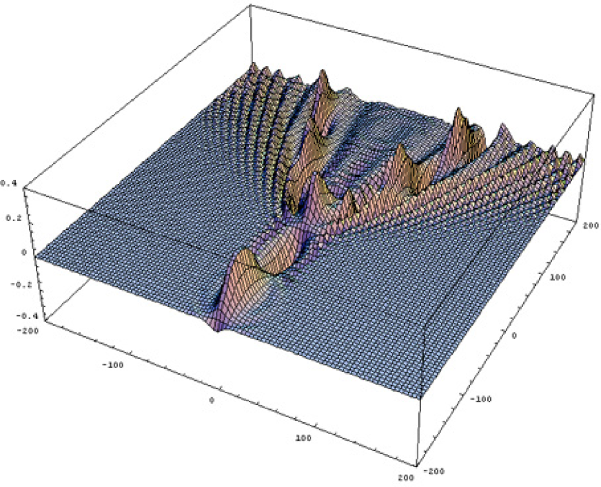
Figure 1: This picture shows the scattering process of one soliton to two solitons for equation (1), where amplitude of external force $\varepsilon=0.1$, $S=0.005t^{2}$, $f=2\sqrt{2}\cosh^{-1}(0.2x)+$ $2\sqrt{2}\exp(0.2ix)\cosh^{-1}(0.2x-5)+$ $2\sqrt{2}\exp(-0.2ix)\cosh^{-1}(0.2x+5),$ initial data is pure soliton of NLSE at $\Psi|_{t=-200}=0.2\sqrt{2}\cosh^{-1}(0.2x)$ , resonance curve is $t=0$.

Let us explain the terms ’scattering’ and ’resonance’ which is used in the work. Usually one says ’scattering’ for process when a wave is changed after obstacle. The same process is studied in our work for solitons which are nonlinear waves of NLSE. The obstacle is a line where the external force has a resonance in the equation for first-order term in the asymptotic solution for perturbed NLSE. Under ’resonance’ we understand standard phenomenon of grows solution because of oscillating external force. The resonance phenomenon takes place in a thin domain near some curve usually called a resonance curve. So we use the term ’local resonance’.

We consider the process of scattering in detail and obtain the connection formula between pre-resonance and post-resonance solutions. In general case the passage through the resonance leads to changing of the number of solitons. This effect is based on the phenomenon of soliton generation due to the passage through the resonance by the external driving force [9].

We found that the scattering of solitary waves on the resonance is a general effect for the wave propagation in a nonlinear media. In this work we investigate this effect for the simplest model. It allows to show the essence of this effect without unnecessary details.

This paper has the following structure. The first section contains the statement of the problem and the main result. The sections 2-4 are reviewed asymptotic analysis of the problem which was developed in [10]. The second section contains the asymptotic construction in the pre-resonance domain. In the third section we construct the asymptotic solution in the neighborhood of the resonance curve. The fourth section of the paper is devoted to construction of the post-resonance asymptotics. Asymptotics are constructed by multiple scale method [11] and matched [12]. At last five section contains the results of numerical simulation which justify the obtained asymptotic formulas.

1 Statement of the problem and result

We study the perturbed NLS equation (1) with a special phase of the driving force: $S/\varepsilon^{2}=\varepsilon^{2}t^{2}$. The amplitude $f=f(\varepsilon x)$ is a smooth and rapidly vanished function. The small parameter in the right hand side of the equation is defined as $\varepsilon^{2}$ only for a convenience.

The goal of our work is the study of a slow evolution of the solution with a small amplitude for the equation (1). In the general case the small amplitude solutions are defined by the linear Schrödinger equation. However there exists a magic relation between scales of independent variables of a carrier wave and an amplitude of its envelope function which leads to the nonlinear Schrödinger equation for the envelope function of the leading-order term of the asymptotics. This relation was observed for different physical problems in pioneer works [1, 2, 3]. An example of such relation give the following substitution

$$\Psi=\varepsilon U(t_{2},x_{1},\varepsilon),\quad t_{2}=\varepsilon^{2}t,\ \ x_{1}=\varepsilon x,$$

then the equation (1) has the form:

$$i\partial_{t_{2}}U+\partial_{x_{1}}^{2}U+|U|^{2}U=\varepsilon^{-1}fe^{iS/\varepsilon^{2}}.$$ (2)

The strong perturbation with rapid phase for NLSE may be considered as a model for the high-frequency heating of plasma [13] and leads to the phenomenon of the scattering of solitons.

It is known if $f\equiv 0$ then there exists a soliton solution of the NLSE. We’ll show that for $f\not\equiv 0$ the number of solitons may be changed due to passage through the resonant curve. The resonant curve defines as a line where the frequency of the driving force is equal to the eigenfrequency of linearized Schródinger equation. In our case this curve is $t=0$. After passage the resonance the number of solitons depends on amplitude of the perturbation on the resonance curve $t=0$.

In the simplest case the phase is linear function with respect to $t$ $S/\varepsilon^{2}=\omega t,\ \omega=\hbox{const}$. In general situation the constant frequency of the driving force does not lead to the scattering of solitons. Let us investigate the driving force with slowly varying frequency. The most simplest dependence on $t$ for $\omega$ has a form $\omega=\varepsilon^{2}t/2$. Hence $S=\varepsilon^{4}t^{2}/2$. Namely the equation with this form of the phase function of the driving force is studied in this work. The amplitude $f$ of the driving force admit an additional dependency on $\varepsilon^{2}t$ but it leads to complicated formulas and no more.

Let us formulate the result of this work. Below we use the following variables $x_{j}=\varepsilon^{j}x,\ t_{j}=\varepsilon^{j}t,\ j=1,2$.

Let the asymptotic solution of (1) be

$$\Psi(x,t,\varepsilon)=\varepsilon\stackrel{{\scriptstyle 1}}{{u}}(x_{1},t_{2})+O(\varepsilon^{2})\quad\mbox{as}\quad-c<t_{2}<0,$$

where $c=\hbox{const}>0$ and $\stackrel{{\scriptstyle 1}}{{u}}(x_{1},t_{2})$ satisfies

$$\partial_{t_{2}}\stackrel{{\scriptstyle 1}}{{u}}+\partial_{x_{1}}^{2}\stackrel{{\scriptstyle 1}}{{u}}+|\stackrel{{\scriptstyle 1}}{{u}}|^{2}\stackrel{{\scriptstyle 1}}{{u}}=0$$

and initial condition

$$\stackrel{{\scriptstyle 1}}{{u}}|_{t_{2}=t^{0}}=h_{1}(x_{1}),\quad t^{0}=\hbox{const}<0.$$

Then in the domain $0<t_{2}<c$ the asymptotic solution of (1) has a form

$$\Psi(x,t,\varepsilon)=\varepsilon\stackrel{{\scriptstyle 1}}{{v}}(x_{1},t_{2})+O(\varepsilon^{2}),$$ (3)

where $\stackrel{{\scriptstyle 1}}{{v}}(x_{1},t_{2})$ is a solution of NLSE with initial condition

$$\stackrel{{\scriptstyle 1}}{{v}}|_{t_{2}=0}=\stackrel{{\scriptstyle 1}}{{u}}(x_{1},0)+(1-i)\sqrt{\pi}f(x_{1}).$$ (4)

Formula (4) is the main result of the paper. This formula connects the main order term $\stackrel{{\scriptstyle 1}}{{u}}$ of the asymptotic solution before the scattering, external driving force $f$ and initial condition $\stackrel{{\scriptstyle 1}}{{v}}$ for the main order term of the asymptotic solution after the scattering. This formula is derived in the end of section 4.

Let us explain the result for soliton solution. If in the domain $-c<t_{2}<0$ the solution has $N$-soliton form then in the domain $0<t_{2}<c$ the number of solitons is defined by initial condition (4).

Given analysis is valid at $|t_{2}|\leq C$, for $\forall C=\hbox{const}$. When $|\varepsilon^{2}t|\gg 1$ the perturbation force will modulate the parameters of the soliton solution, see [6, 7].

2 Incident wave

In this section we construct the asymptotic solution of equation (1) in pre-resonance domain. This solution contains two parts. The first part is a specific solution of the nonhomogeneous equation. This solution oscillates with the frequency of the driving force. The amplitudes are determined by an algebraic equations. The second part of the solution is a solution of the homogeneous equation. The solution contains an undefined function due to integration. This undefined function usually determines by initial condition for the Cauchy problem.

We construct the formal asymptotic solution in the WKB-like form

$$\Psi(x,t,\varepsilon)=\varepsilon\stackrel{{\scriptstyle 1}}{{u}}(x_{1},t_{2})+\varepsilon^{3}\stackrel{{\scriptstyle 3}}{{u}}(x_{1},t_{2})+\varepsilon^{2}\stackrel{{\scriptstyle 2}}{{B}}(x_{1},t_{2})\exp(iS/\varepsilon^{2})+$$

$$\varepsilon^{4}\bigg{(}\stackrel{{\scriptstyle 4}}{{B}}_{1}(x_{1},t_{2})\exp(iS/\varepsilon^{2})+\stackrel{{\scriptstyle 4}}{{B}}_{-1}(x_{1},t_{2})\exp(-iS/\varepsilon^{2})\bigg{)}$$ (5)

$$+\varepsilon^{5}\stackrel{{\scriptstyle 5}}{{B}}_{2}(x_{1},t_{2})\exp(2iS/\varepsilon^{2}).$$

To determine the coefficients of the asymptotics substitute (5) into equation (1). It yields

$$\varepsilon^{2}\bigg{(}-S^{\prime}\stackrel{{\scriptstyle 2}}{{B}}-f\bigg{)}\exp(iS/\varepsilon^{2})+\varepsilon^{3}\bigg{(}i\stackrel{{\scriptstyle 1}}{{u}}_{t_{2}}+\stackrel{{\scriptstyle 1}}{{u}}_{x_{1}x_{1}}+|\stackrel{{\scriptstyle 1}}{{u}}|^{2}\stackrel{{\scriptstyle 1}}{{u}}\bigg{)}$$

$$+\varepsilon^{4}\bigg{(}\bigg{(}-S^{\prime}\stackrel{{\scriptstyle 4}}{{B}}_{1}+i\stackrel{{\scriptstyle 2}}{{B}}_{t_{2}}+\stackrel{{\scriptstyle 2}}{{B}}_{x_{1}x_{1}}+2|\stackrel{{\scriptstyle 1}}{{u}}|{}^{2}\stackrel{{\scriptstyle 2}}{{B}}\bigg{)}\exp(iS/\varepsilon^{2})+$$

$$+\bigg{(}S^{\prime}\stackrel{{\scriptstyle 4}}{{B}}_{-1}+\stackrel{{\scriptstyle 1}}{{u}}{}^{2}\stackrel{{\scriptstyle 2}}{{B}}{}^{*}\bigg{)}\exp(-iS/\varepsilon^{2})\bigg{)}$$

$$\varepsilon^{5}\bigg{(}i\stackrel{{\scriptstyle 3}}{{u}}_{t_{2}}+\stackrel{{\scriptstyle 3}}{{u}}_{x_{1}x_{1}}+2|\stackrel{{\scriptstyle 1}}{{u}}|^{2}\stackrel{{\scriptstyle 3}}{{u}}+\stackrel{{\scriptstyle 1}}{{u}}{}^{2}\stackrel{{\scriptstyle 3}}{{u}}{}^{*}+2\stackrel{{\scriptstyle 1}}{{u}}|\stackrel{{\scriptstyle 2}}{{B}}|{}^{2}+$$

$$\bigg{(}-2S^{\prime}\stackrel{{\scriptstyle 5}}{{B}}_{2}+\stackrel{{\scriptstyle 1}}{{u}}{}^{*}\stackrel{{\scriptstyle 2}}{{B}}{}^{2}\bigg{)}\exp(2iS/\varepsilon^{2})\bigg{)}=\varepsilon^{6}R(t_{2},x_{1}).$$

The residue part of the asymptotics has a form

$$R(t_{2},x_{1})=O(|\stackrel{{\scriptstyle 2}}{{B}}|^{3}+\varepsilon^{3}|\stackrel{{\scriptstyle 3}}{{u}}|^{3}+\varepsilon^{6}|\stackrel{{\scriptstyle 4}}{{B}}_{1}|^{3}+\varepsilon^{6}|\stackrel{{\scriptstyle 4}}{{B}}_{-1}|^{3}+\varepsilon^{9}|\stackrel{{\scriptstyle 5}}{{B}}_{2}|^{3}).$$ (6)

Collect the terms with the same order of $\varepsilon$ up to the order of $\varepsilon^{5}$ and reduce similar terms. It yields differential equations for $\stackrel{{\scriptstyle 1}}{{u}},\stackrel{{\scriptstyle 3}}{{u}}$ and algebraic equations for $\stackrel{{\scriptstyle 2}}{{B}}$, $\stackrel{{\scriptstyle 4}}{{B}}_{\pm 1}$ and $\stackrel{{\scriptstyle 5}}{{B}}_{2}$.

$$i\stackrel{{\scriptstyle 1}}{{u}}_{t_{2}}+\stackrel{{\scriptstyle 1}}{{u}}_{x_{1}x_{1}}+|\stackrel{{\scriptstyle 1}}{{u}}|^{2}\stackrel{{\scriptstyle 1}}{{u}}=0,$$ (7)

$$i\stackrel{{\scriptstyle 3}}{{u}}_{t_{2}}+\stackrel{{\scriptstyle 3}}{{u}}_{x_{1}x_{1}}+2|\stackrel{{\scriptstyle 1}}{{u}}|^{2}\stackrel{{\scriptstyle 3}}{{u}}+\stackrel{{\scriptstyle 1}}{{u}}{}^{2}\stackrel{{\scriptstyle 3}}{{u}}{}^{*}=-2|\stackrel{{\scriptstyle 2}}{{B}}|^{2}\stackrel{{\scriptstyle 1}}{{u}},$$ (8)

$$-S^{\prime}\stackrel{{\scriptstyle 2}}{{B}}=f,$$ (9)

$$-S^{\prime}\stackrel{{\scriptstyle 4}}{{B}}_{1}=i\stackrel{{\scriptstyle 2}}{{B}}_{t_{2}}+\stackrel{{\scriptstyle 2}}{{B}}_{x_{1}x_{1}}+|\stackrel{{\scriptstyle 1}}{{u}}|^{2}\stackrel{{\scriptstyle 2}}{{B}},$$ (10)

$$S^{\prime}\stackrel{{\scriptstyle 4}}{{B}}_{-1}=-\stackrel{{\scriptstyle 1}}{{u}}{}^{2}\stackrel{{\scriptstyle 2}}{{B}}{}^{*},$$ (11)

$$-2S^{\prime}\stackrel{{\scriptstyle 5}}{{B}}_{2}=\stackrel{{\scriptstyle 1}}{{u}}{}^{*}\stackrel{{\scriptstyle 2}}{{B}}{}^{2}.$$ (12)

The functions $\stackrel{{\scriptstyle 1}}{{u}},\stackrel{{\scriptstyle 3}}{{u}}$ are uniquely determined by initial conditions at the moment $t_{2}=t^{0}$. We suppose that $t^{0}=\hbox{const}<0$ and

$$\stackrel{{\scriptstyle 1}}{{u}}|_{t_{2}=t^{0}}=h_{1}(x_{1});\quad\stackrel{{\scriptstyle 3}}{{u}}|_{t_{2}=t^{0}}=h_{3}(x_{1});$$

where functions $h_{1},h_{3}$ are smooth and rapidly vanish as $|x_{1}|\to\pm\infty$.

It’s known the solutions $\stackrel{{\scriptstyle 1}}{{u}}$ and $\stackrel{{\scriptstyle 3}}{{u}}$ exist for bounded values of $t_{2}$, see [14, 15].

Remark The solution of the equation for $\stackrel{{\scriptstyle 3}}{{u}}$ contains growing terms as $t_{2}\to\infty$, see for example [15]. These terms are secular as $t_{2}\sim\varepsilon^{-1}$. But we do not consider such long times in this work.

The coefficients of the representation (5) have a singularity as $S^{\prime}\to 0$. The order of singularity of $\stackrel{{\scriptstyle j}}{{B}}_{k}$ is easy calculated.

$$\stackrel{{\scriptstyle 2}}{{B}}=O(t^{-1}),\quad\stackrel{{\scriptstyle 4}}{{B}}_{1}=O(t^{-3}).$$

To determine the asymptotics of $\stackrel{{\scriptstyle 3}}{{u}}$ as $t_{2}\to-0$ we construct the solution of the form

$$\stackrel{{\scriptstyle 3}}{{u}}=t_{2}^{-1}\stackrel{{\scriptstyle 3}}{{u}}{}^{(-1,0)}(x_{1},t_{2})+\ln|t_{2}|\stackrel{{\scriptstyle 3}}{{u}}{}^{(0,1)}(x_{1},t_{2})+t_{2}\ln|t_{2}|\stackrel{{\scriptstyle 3}}{{u}}{}^{(1,1)}(x_{1},t_{2})+\widehat{\stackrel{{\scriptstyle 3}}{{u}}}(x_{1},t_{2}).$$ (13)

Substitute this representation into equation (8) and collect the terms of the same order with respect to $t_{2}$. It yields equations for coefficients of the asymptotics (13)

$$\stackrel{{\scriptstyle 3}}{{u}}{}^{(-1,0)}=i2|f|^{2}\stackrel{{\scriptstyle 1}}{{u}},$$

$$\stackrel{{\scriptstyle 3}}{{u}}{}^{(0,1)}=-iL(\stackrel{{\scriptstyle 3}}{{u}}{}^{(-1,0)}),$$

$$\stackrel{{\scriptstyle 3}}{{u}}{}^{(1,1)}=-iL(\stackrel{{\scriptstyle 3}}{{u}}{}^{(0,1)}),$$

$$L(\widehat{\stackrel{{\scriptstyle 3}}{{u}}})=it_{2}\ln|t_{2}|L(\stackrel{{\scriptstyle 3}}{{u}}{}^{(1,1)})+i\stackrel{{\scriptstyle 3}}{{u}}{}^{(1,1)}.$$ (14)

Here $L(u)$ is a linear operator of the form

$$L(u)=i\partial_{t_{2}}u+\partial_{x_{1}}^{2}u+2|\stackrel{{\scriptstyle 1}}{{u}}|^{2}u+\stackrel{{\scriptstyle 1}}{{u}}{}^{2}u^{*}.$$

Functions $\stackrel{{\scriptstyle 3}}{{u}}{}^{(-1,0)}$, $\stackrel{{\scriptstyle 3}}{{u}}{}^{(0,1)}$ and $\stackrel{{\scriptstyle 3}}{{u}}{}^{(1,1)}$ are determined from algebraic equations. These functions are bounded as $-\hbox{const}<t_{2}\leq 0,\ \hbox{const}>0$.

The function $\widehat{\stackrel{{\scriptstyle 3}}{{u}}}$ is a solution of nonhomogeneous linearized Schrodinger equation. The right hand side of the equation is a smooth function as $-\hbox{const}<t_{2}\leq 0,\ \hbox{const}>0$. The solution of this equation can be obtained using results of [15]. In particularly if $\stackrel{{\scriptstyle 1}}{{u}}$ is N-solitons solution of NLSE then exists the bounded solution of nonhomogeneous linearized Schrodinger equation (14) as $-\hbox{const}<t_{2}\leq 0,\ \hbox{const}>0$.

The asymptotic form (5) allows to solve equation (1) up to the order $\varepsilon^{6}$. To obtain more accurate approximation one have to include terms without fast oscillating of the order $o(\varepsilon^{3})$ into asymptotic solution (5). Therefore we define the domain of validity of (5) by following relation:

$$\varepsilon^{6}R(t_{2},x_{1})=o(\varepsilon^{3}),\quad\varepsilon\to 0.$$

Coefficients of (5) have singularity at $t_{2}=0$. The residue part increases as $t_{2}\to 0$. From formulas (6) and (7)–(12) one can easily obtain the behaviour of the residue part:

$$R(t_{2},x_{1})=O(t_{2}^{-3}+\varepsilon^{6}t_{2}^{-9}),\quad t_{2}\to-0.$$

It yields the domain of validity of (5)

$$-t_{2}\gg\varepsilon\quad\hbox{or}\quad-t\gg\varepsilon^{-1}.$$

3 Scattering

In the neighborhood of the point $t_{2}=0$ the frequency of the driving force becomes resonant. Formally it means representation (5) is not valid.

In this part of the work we construct another representation for the solution of equation (1). This representation is valid in the neighborhood of the resonance line $t_{2}=0$.

$$\Psi(x,t,\varepsilon)=\varepsilon\stackrel{{\scriptstyle 1}}{{w}}(x_{1},t_{1})\big{)}+\varepsilon^{2}\stackrel{{\scriptstyle 2}}{{w}}(x_{1},t_{1})+$$

$$\varepsilon^{3}\ln\varepsilon\stackrel{{\scriptstyle 3,1}}{{w}}(x_{1},t_{1})+\varepsilon^{3}\stackrel{{\scriptstyle 3}}{{w}}(x_{1},t_{1})\qquad\varepsilon\to 0.$$ (15)

Here we use a new scaled variable $t_{1}=t_{2}/\varepsilon$. Representation (15) is matched with (5). It means these formulas are equivalent up to value $o(\varepsilon^{5})$ as $t_{2}\to-0$. The coefficients of (15) are determined by ordinary differential equations (16), (18), (20) and matching conditions.

To obtain the behaviour of the coefficients of (15) as $t_{1}\to-\infty$ match (15) with (5). Write (5) in terms of $t_{1}$

$$\Psi(x,t,\varepsilon)=\varepsilon\bigg{(}\stackrel{{\scriptstyle 1}}{{u}}(x_{1},0)-\big{(}t_{1}^{-1}f+it_{1}^{-3}f\big{)}\exp(iS/\varepsilon^{2})\bigg{)}+$$

$$\varepsilon^{2}\bigg{(}\partial_{t_{2}}\stackrel{{\scriptstyle 1}}{{u}}(x_{1},t_{2})|_{t_{2}=0}t_{1}+t_{1}^{-1}i|f|^{2}\stackrel{{\scriptstyle 1}}{{u}}(x_{1},0)+O\big{(}t_{1}^{-2}\big{)}\bigg{)}+$$

$$\varepsilon^{3}\ln\varepsilon\bigg{(}-iL(2i|f|^{2}\stackrel{{\scriptstyle 1}}{{u}})|_{t_{2}=0}+o(1)\bigg{)}+$$

$$+\varepsilon^{3}\bigg{(}{1\over 2}\partial_{t_{2}}^{2}\stackrel{{\scriptstyle 1}}{{u}}(x_{1},t_{2})|_{t_{2}=0}t_{1}^{2}+\widehat{\stackrel{{\scriptstyle 3}}{{u}}}(x_{1},0)+o(1)\bigg{)},\quad 1\ll-t_{1}\ll\varepsilon^{-1},\,\,\varepsilon\to 0.$$

To obtain equations for coefficients of (15) substitute (15) into equation (1). It yields

$$\varepsilon^{2}\bigg{(}(\partial_{t_{1}}\stackrel{{\scriptstyle 1}}{{w}}-f\exp(iS/\varepsilon^{2})\bigg{)}+\varepsilon^{3}\bigg{(}\partial_{t_{1}}\stackrel{{\scriptstyle 2}}{{w}}+\partial_{x_{1}}^{2}\stackrel{{\scriptstyle 1}}{{w}}+\gamma|\stackrel{{\scriptstyle 1}}{{w}}|\stackrel{{\scriptstyle 1}}{{w}}\bigg{)}+$$

$$\varepsilon^{4}\bigg{(}\partial_{t_{1}}\stackrel{{\scriptstyle 3}}{{w}}+\partial_{x_{1}}^{2}\stackrel{{\scriptstyle 2}}{{w}}++\stackrel{{\scriptstyle 1}}{{w}}{}^{2}\stackrel{{\scriptstyle 2}}{{w}}{}^{*}+2\gamma|\stackrel{{\scriptstyle 1}}{{w}}|\stackrel{{\scriptstyle 2}}{{w}}\bigg{)}=\varepsilon^{5}\rho(t_{1},x_{1},\varepsilon).$$

The function $\rho(t_{1},x_{1},\varepsilon)$ can be represented in the form

$$\rho(t_{1},x_{1},\varepsilon)=O(|\stackrel{{\scriptstyle 1}}{{w}}|^{2}\stackrel{{\scriptstyle 3}}{{w}}+\partial_{x_{1}}^{2}\stackrel{{\scriptstyle 3}}{{w}}+\varepsilon|\stackrel{{\scriptstyle 2}}{{w}}|^{3}+\varepsilon^{4}|\stackrel{{\scriptstyle 3}}{{w}}|^{3}).$$

Collect the terms of the same order with respect to $\varepsilon$. As result we obtain the equations for coefficients of (15).

$$i\partial_{t_{1}}\stackrel{{\scriptstyle 1}}{{w}}=f\exp(it_{1}^{2}/2).$$ (16)

The matching conditions give $\stackrel{{\scriptstyle 1}}{{w}}=\stackrel{{\scriptstyle 1}}{{u}}(x_{1},0)\,\,\,t_{1}\to-\infty$. The solution of this problem is represented in terms of Fresnel integral

$$\stackrel{{\scriptstyle 1}}{{w}}=\stackrel{{\scriptstyle 1}}{{u}}(x_{1},0)-if(x_{1})\int_{-\infty}^{t_{1}}\exp(i\theta^{2}/2)d\theta.$$ (17)

Equations for higher-order terms are

$$i\partial_{t_{1}}\stackrel{{\scriptstyle 2}}{{w}}=-\partial_{x_{1}}^{2}\stackrel{{\scriptstyle 1}}{{w}}+|\stackrel{{\scriptstyle 1}}{{w}}|^{2}\stackrel{{\scriptstyle 1}}{{w}},$$ (18)

$$i\partial_{t_{1}}\stackrel{{\scriptstyle 3,1}}{{w}}=0,$$ (19)

$$i\partial_{t_{1}}\stackrel{{\scriptstyle 3}}{{w}}=-\partial_{x_{1}}^{2}\stackrel{{\scriptstyle 2}}{{w}}-2|\stackrel{{\scriptstyle 1}}{{w}}|^{2}\stackrel{{\scriptstyle 2}}{{w}}-\stackrel{{\scriptstyle 1}}{{w}}{}^{2}\stackrel{{\scriptstyle 2}}{{w}}{}^{*}.$$ (20)

The higher-order terms satisfy fist order ordinary differential equations with respect to $t_{1}$. The spatial variable $x_{1}$ is a parameter in these equations. The solutions of these equation are uniquely defined by terms of the order of $1$ in asymptotics as $t_{1}\to-\infty$. The asymptotics as $t_{1}\to-\infty$ is obtained by matching

$$\stackrel{{\scriptstyle 2}}{{w}}=\partial_{t_{2}}\stackrel{{\scriptstyle 1}}{{u}}(x_{1},t_{2})|_{t_{2}=0}t_{1}+o(1);$$

$$\stackrel{{\scriptstyle 3,1}}{{w}}=-iL(2i|f|^{2}\stackrel{{\scriptstyle 1}}{{u}})|_{t_{2}=0}+o(1),$$

$$\stackrel{{\scriptstyle 3}}{{w}}={1\over 2}\partial_{t_{2}}^{2}\stackrel{{\scriptstyle 1}}{{u}}(x_{1},t_{2})|_{t_{2}=0}t_{1}^{2}+\widehat{\stackrel{{\scriptstyle 3}}{{u}}}(x_{1},0)+o(1).$$

To determine the behaviour of the solution after resonance we need to calculate the asymptotics as $t_{1}\to+\infty$ of the coefficients for representation (15). Calculations give

$$\stackrel{{\scriptstyle 1}}{{w}}(x_{1},t_{1})=\stackrel{{\scriptstyle 1}}{{u}}(x_{1},0)-if(x_{1})\bigg{[}ic_{1}+{\exp(it_{1}^{2}/2)\over it_{1}}+O(t_{1}^{-3})\bigg{]},$$

where $c_{1}=(1-i)\sqrt{\pi}$.

Denote by

$$\stackrel{{\scriptstyle 1}}{{w}}(x_{1},t_{1})|_{t_{1}\to\infty}=\stackrel{{\scriptstyle 1}}{{w}}_{0}(x_{1}).$$

The function $\stackrel{{\scriptstyle 2}}{{w}}(x_{1},t_{1})$ has the asymptotics of the form

$$\stackrel{{\scriptstyle 2}}{{w}}(x_{1},t_{1})=t_{1}\stackrel{{\scriptstyle 2}}{{w}}{}_{1}(x_{1})+\stackrel{{\scriptstyle 2}}{{w}}{}_{0}(x_{1})+g_{1}(x_{1}){\exp(it_{1}^{2}/2)\over it_{1}^{2}}+O(t_{1}^{-4}),$$

where

$$\stackrel{{\scriptstyle 2}}{{w}}{}_{1}=-\partial_{x_{1}}^{2}\stackrel{{\scriptstyle 1}}{{w}}_{0}+|\stackrel{{\scriptstyle 1}}{{w}}_{0}|^{2}\stackrel{{\scriptstyle 1}}{{w}};$$

$$\stackrel{{\scriptstyle 2}}{{w}}{}_{0}(x_{1})=\lim_{t_{1}\to\infty}\bigg{(}\int_{-\infty}^{t_{1}}\big{[}\partial_{x_{1}}^{2}\stackrel{{\scriptstyle 0}}{{w}}(x_{1},\theta)+|\stackrel{{\scriptstyle 0}}{{w}}(x_{1},\theta)|^{2}\stackrel{{\scriptstyle 0}}{{w}}(x_{1},\theta)\big{]}d\theta-\stackrel{{\scriptstyle 2}}{{w}}_{1}t_{1}\bigg{)},$$

$g_{1}(x_{1})=k_{1}\partial_{x_{1}}f+k_{2}|f|^{2}f$, $k_{1}$ and $k_{2}$ are constants.

$$\stackrel{{\scriptstyle 3}}{{w}}(x_{1},t_{1})=t_{1}^{2}\stackrel{{\scriptstyle 3}}{{w}}{}_{2}(x_{1})+o(t_{1}^{2}),\quad t_{1}\to\infty,$$

where

$$\stackrel{{\scriptstyle 3}}{{w}}{}_{2}(x_{1})=i\left(\partial_{x_{1}}^{2}\stackrel{{\scriptstyle 2}}{{w}}_{1}+2|\stackrel{{\scriptstyle 1}}{{w}}_{0}|^{2}\stackrel{{\scriptstyle 2}}{{w}}_{1}+\stackrel{{\scriptstyle 1}}{{w}}{}_{0}^{2}\stackrel{{\scriptstyle 2}}{{w}}{}_{1}^{*}\right),$$

The domain of validity for (15) is defined by the same way as was shown in previous section. We require the following relation is valid

$$\varepsilon^{5}\rho(t_{1},x_{1},\varepsilon)=o(\varepsilon^{2}),\quad t_{1}\to\infty.$$

The determined above behaviour of coefficients of asymptotics (15) give the domain of validity for (15)

$$|t_{1}|\ll\varepsilon^{-1}\quad\hbox{or}\quad|t|\ll\varepsilon^{-2}.$$

4 Scattered wave

In this section we construct the asymptotic solution of equation (1) after passage through the resonance. The leading-order term of the solution satisfies NLSE and depends on $x_{1},t_{2}$ as well as before resonance. But this leading-order term is determined by another solution of NLSE which contains generally speaking another number of solitons.

We construct the asymptotic solution of the form

$$\Psi(x,t,\varepsilon)=\varepsilon\stackrel{{\scriptstyle 1}}{{v}}(x_{1},t_{2})+\varepsilon^{2}\stackrel{{\scriptstyle 2}}{{v}}(x_{1},t_{2})+$$

$$\varepsilon^{2}\stackrel{{\scriptstyle 2}}{{A}}(t_{2},x_{1})\exp(iS/\varepsilon^{2})+\varepsilon^{4}(\stackrel{{\scriptstyle 4}}{{A}}_{1}(t_{2},x_{1})\exp(iS/\varepsilon^{2})+$$

$$\stackrel{{\scriptstyle 4}}{{A}}_{-1}(t_{2},x_{1})\exp(-iS/\varepsilon^{2})).$$ (21)

Substitute this representation into (1):

$$\varepsilon^{2}(-S^{\prime}\stackrel{{\scriptstyle 2}}{{A}}-f)\exp(iS/\varepsilon^{2})+\varepsilon^{3}(\partial_{t_{2}}\stackrel{{\scriptstyle 1}}{{v}}+\partial_{x_{1}}^{2}\stackrel{{\scriptstyle 1}}{{v}}+|\stackrel{{\scriptstyle 1}}{{v}}|^{2}\stackrel{{\scriptstyle 1}}{{v}})+$$

$$\varepsilon^{4}(\partial_{t_{2}}\stackrel{{\scriptstyle 2}}{{v}}+\partial_{x_{1}}^{2}\stackrel{{\scriptstyle 2}}{{v}}+2|\stackrel{{\scriptstyle 1}}{{v}}|^{2}\stackrel{{\scriptstyle 2}}{{v}}+\stackrel{{\scriptstyle 1}}{{v}}^{2}\stackrel{{\scriptstyle 2}}{{v}}{}^{*}+$$

$$(-S^{\prime}\stackrel{{\scriptstyle 4}}{{A}}_{1}+\partial_{t_{2}}\stackrel{{\scriptstyle 2}}{{A}}+\partial_{x_{1}}^{2}\stackrel{{\scriptstyle 2}}{{A}}+2|\stackrel{{\scriptstyle 1}}{{v}}|^{2}\stackrel{{\scriptstyle 2}}{{A}})\exp(iS/\varepsilon^{2})+$$

$$(S^{\prime}\stackrel{{\scriptstyle 4}}{{A}}_{-1}+\stackrel{{\scriptstyle 1}}{{v}}{}^{2}\stackrel{{\scriptstyle 2}}{{A}}{}^{*})\exp(-iS/\varepsilon^{2}))=\varepsilon^{5}r(t_{2},x_{1},\varepsilon).$$

Here $r(t_{2},x_{1},\varepsilon)$ depends on coefficients of the asymptotics (21). This dependence is easy calculated. The coefficients $\stackrel{{\scriptstyle 2}}{{A}}$, $\stackrel{{\scriptstyle 4}}{{A}}_{1}$ and $\stackrel{{\scriptstyle 4}}{{A}}_{-1}$ have singularity on the resonance curve. To determine the domain of validity of (21) we need to derive the explicit formula for $r$

$$r(t_{2},x_{1},\varepsilon)=O(1+\varepsilon|\stackrel{{\scriptstyle 2}}{{A}}|^{3}+\varepsilon\ln|\varepsilon|+\varepsilon^{7}(|\stackrel{{\scriptstyle 4}}{{A}}_{1}|^{3}+|\stackrel{{\scriptstyle 4}}{{A}}_{-1}|^{3})).$$

Collect the terms of the same order of small parameter and the same exponents. It yields the equations for coefficients of representation (21).

$$\partial_{t_{2}}\stackrel{{\scriptstyle 1}}{{v}}+\partial_{x_{1}}^{2}\stackrel{{\scriptstyle 1}}{{v}}+|\stackrel{{\scriptstyle 1}}{{v}}|^{2}\stackrel{{\scriptstyle 1}}{{v}}=0;$$ (22)

$$\partial_{t_{2}}\stackrel{{\scriptstyle 2}}{{v}}+\partial_{x_{1}}^{2}\stackrel{{\scriptstyle 2}}{{v}}+2|\stackrel{{\scriptstyle 1}}{{v}}|^{2}\stackrel{{\scriptstyle 2}}{{v}}+\stackrel{{\scriptstyle 1}}{{v}}{}^{2}\stackrel{{\scriptstyle 2}}{{v}}{}^{*}=0$$ (23)

$$-S^{\prime}\stackrel{{\scriptstyle 2}}{{A}}=f;$$

$$-S^{\prime}\stackrel{{\scriptstyle 4}}{{A}}_{1}=-\partial_{t_{2}}\stackrel{{\scriptstyle 2}}{{A}}-\partial_{x_{1}}^{2}\stackrel{{\scriptstyle 2}}{{A}}-2|\stackrel{{\scriptstyle 1}}{{v}}|^{2}\stackrel{{\scriptstyle 2}}{{A}};$$

$$S^{\prime}\stackrel{{\scriptstyle 4}}{{A}}_{-1}=-\stackrel{{\scriptstyle 1}}{{v}}{}^{2}\stackrel{{\scriptstyle 2}}{{A}}{}^{*}.$$

Initial conditions for differential equations for $\stackrel{{\scriptstyle 1}}{{v}}$ are obtained by matching. These conditions are evaluated on the resonance curve $t_{0}=0$.

$$\stackrel{{\scriptstyle 1}}{{v}}|_{t_{2}=0}=\stackrel{{\scriptstyle 1}}{{u}}(x_{1},0)+(1-i)\sqrt{\pi}f(x_{1});$$ (24)

$$\stackrel{{\scriptstyle 2}}{{v}}|_{t_{2}=0}=\stackrel{{\scriptstyle 2}}{{w}}_{0}(x_{1}).$$ (25)

The residue part $\varepsilon^{5}r(t_{2},x_{1},\varepsilon)=o(\varepsilon^{2})$ as $t_{2}\gg\varepsilon$. This condition is determined the domain of validity for (21).

Formula (24) is connection formula for the leading-order term of the asymptotic solution before and after the resonance. Additional term $(1-i)\sqrt{\pi}f(x_{1})$ leads to changing of the solution after passage through the resonance.

5 Numerical justification of asymptotic analysis

In this section we justify our asymptotic formula (4). Let us consider the pure soliton initial condition for equation (1):

$$\Psi(x,t,\varepsilon)|_{t=t_{0}}={{2\sqrt{2}\varepsilon\eta\exp\{-i2c\varepsilon x-4(c^{2}-\eta^{2})t_{0}\varepsilon^{2}\}}\over{\cosh(2\eta\varepsilon x+8c\eta\varepsilon^{2}t_{0}+s)}}$$ (26)

According of our analytical results this initial condition leads to one soliton solution as the leading-order term of the asymptotic solution:

$$\stackrel{{\scriptstyle 1}}{{u}}(x_{1},t_{2})={{2\sqrt{2}\eta\exp\{-i2cx_{1}-4i(c^{2}-\eta^{2})t_{2}\}}\over{\cosh(2\eta x_{1}+8c\eta t_{2}+s)}}.$$

This soliton propagates up to the resonance curve $t=0$.

To annihilate this soliton on the resonance curve one may choose the specific form of the amplitude of the perturbation such that the left hand side of relation (4) equals zero:

$$0=\stackrel{{\scriptstyle 1}}{{u}}(x_{1},0)+(1-i)\sqrt{\pi}f(x_{1}).$$

Hence

$$f(x_{1})={-(1+i)\over 2\sqrt{\pi}}\stackrel{{\scriptstyle 1}}{{u}}(x_{1},0)={-(1+i)\over\sqrt{\pi}}{{\sqrt{2}\eta\exp\{-i2cx_{1}\}}\over{\cosh(2\eta x_{1}+s)}}$$

To illustrate this by numerical simulations we choose $\varepsilon=0.1,\eta=1,s=0,c=0,t^{0}=-200$. Then the original equation (1) has the form

$$i\partial_{t}\Psi+\partial_{x}^{2}\Psi+|\Psi|^{2}\Psi=0.01f\exp\{i0.005t^{2}\}.$$

Initial condition is

$$\Psi|_{t=-200}={0.2\sqrt{2}\over{\cosh(0.2x)}},$$

and amplitude of the perturbation is

$$f={-(1+i)\over\sqrt{\pi}}{{\sqrt{2}}\over{\cosh(0.2x)}}$$

The numerical simulations of annihilation process for soliton of NLSE are presented on the following figure. This justifies the formulas obtained above by matching method.

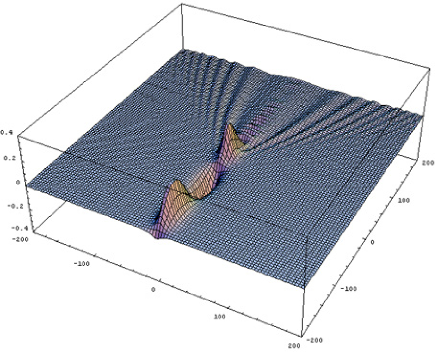
Figure 2: Annihilation of soliton.

6 Summary

We have studied the scattering process on the resonance and obtained the way for the control the parameters of scattered solitons. Using formula (4) one can choose the form of the perturbation to obtain the scattered pattern of the given form. The process of the scattering on the local resonance is an universal phenomenon for waves propagate in dispersion media. We believe that our work can be useful for further understanding and description of solitary waves evolution under perturbation.

Acknowledgments. We are grateful to I.V. Barashenkov, L.A. Kalyakin and B.I.Suleimanov for helpful comments. This work was supported by RFBR 03-01-00716, grant for Sci. Schools 1446.2003.1 and INTAS 03-51-4286.

References

• [1] Kelley P.L. Self-focusing of optical beams. Phys.Rev.Lett., 1965, v.15, 1005-1008.
• [2] Talanov V.I. O samofokusirovke malykh puchkov v nelineinykh sredakh, Pis’ma v ZhETF, 1965, n2, 218-222.
• [3] Zakharov V.E. Ustoichivost’ periodicheskikh voln s konechnoi amplitudoi na poverkhnosti glubokoi zhidkosti. Zhurnal prikladnoi mekhaniki i tekhnicheskoi fiziki, 1968, n2, 86-94.
• [4] Zakharov V.E., Manakov S.V., Novikov S.P., Pitaevskii L.P. Teoriya solitonov: metod obratnoi zadachi. M.:Nauka, 1980.
• [5] Lugiato L.A. and Lefever R., Spatial Dissipative Structures in Passive Optical Systems. Phys. Rev. Lett. 58, 2209 (1987).
• [6] Kaup D.J. A perturbation expansion for the Zakharov-Shabat inverse scattering transform. SIAM J.on Appl.Math., 1976, v. 31, 121–133.
• [7] Karpman V.I., Maslov E.I. Teoriia vozmusheniy dlia solitonov ZhETPh, 1977, t.73, 537–559.
• [8] I.V. Barashenkov, E.V. Zemlyanaya, Existence threshold for the ac-driven damped nonlinear Schrodinger solitons, arXiv:patt-sol/9906001 v1 28 May 1999.
• [9] Glebov S.G., Kiselev O.M., Lazarev V.A. Birth of soliton during passage through local resonance. Proceedings of Steklov Mathematical Institute. Suppl.1, 2003, S84-S90.
• [10] Kiselev O.M., Glebov S.G. Scattering of solitons on resonance. ArXiv:math-ph/0403038.
• [11] Jeffrey A. and Kawahara T. Asymptotic methods in nonlinear wave theory. Pitman Publishing INC, 1982.
• [12] Il’in A.M. Matching of Asymptotic Expansions of Solutions of Boundary Value Problem, AMS, 1992.
• [13] Petviashvili V.I., Pokhotelov O.A. Uedinennye volny v plazme i atmosfere. M.: Energoatomizdat, 1989.
• [14] Dodd R.K., Eilbeck J.C., Gibbon J.D., Morris H.C., Solitons and nonlinear wave equations. Academic Press, 1984.
• [15] Keener J.P., McLaughlin D.W., Solitons under perturbation. Phys. Rev. A. 1977, v.16, N2. 777-790.