Pattern formation by boundary forcing in convectively unstable, oscillatory media with and without differential transport

Abstract

Motivated by recent experiments and models of biological segmentation, we analyze the excitation of pattern-forming instabilities in convectively unstable reaction-diffusion-advection systems, occuring by constant or periodic forcing at the upstream boundary. Such boundary-controlled pattern selection is a generalization of the flow-distributed-oscillation (FDO) mechanism that can be modified to include differential diffusion (Turing) and differential flow (DIFI) modes. Our goal is to clarify the relationships among these mechanisms in the general case where there is differential flow as well as differential diffusion. We do so by analyzing the dispersion relation for linear perturbations and showing how its solutions are affected by differential transport. We find a close relationship between DIFI and FDO modes, while the Turing mechanism gives rise to a distinct set of unstable modes. Finally, we illustrate the relevance of the dispersion relations using nonlinear simulations and we discuss experimental implications of our results.

I Introduction

Recently,  theoretical Andresen -Vasquez and experimental Kaern1 ,Bamforth3 -Santiago attention has been focused on spatiotemporal instabilities in one-dimensional reactive flows.  Among these pattern-forming instabilities are the differential flow (DIFI)Rovinsky92 Rovinsky93 MRDIFI Wu , TuringTuring Kapral , and the physically distinct flow-distributed oscillation (FDO)Andresen Kaern1 Kaern4 Kaern5 Faraday mechanisms. Two of these, DIFI and FDO, necessarily involve a flow, while Turing and DIFI necessarily involve the differential transport of activator and inhibitor species.

Instabilities in a flowing medium may be absolute or convective.Andresen Bamforth1 Proctor Deissler .  In the first case, a localized disturbance grows with time and spreads both upstream and downstream.  In the convective case, on the other hand,  a localized disturbance can not propagate upstream, and so the effect of a temporary localized perturbation is eventually washed downstream and out of the system if there is a downstream boundary.   However, persistent disturbances upstream can have a large effect on the downstream behavior.   This leads to the possibility of noise-sustained structuresProctor Deissler or patterns which are controlled primarily by the upstream boundary conditions. We are insterested here in this latter case, where the upstream boundary is crucial to the control of the pattern.  FDO is a convective mechanism of pattern formation whereby an open flow maps the temporal dynamics of an oscillating medium, whose phase is set at the upstream boundary, onto space.  In the limit of vanishing diffusion, the resulting stationaryAndresen Bamforth1 Bamforth2 Kaern1 Kaern5 , travellingKaern1 Kaern2 Kaern5 and pulsatingKaern2 Kaern5 waves are simple kinematic phase wavesKaern1 , making FDO conceptually the simplest of the pattern-forming mechanisms, although it was discovered later than the others.  The Turing instability, by contrast, was initially conceived of as an absolute instability of a stationary reaction-diffusion medium.  In a flow system, however, Turing Faraday and DIFI RazvanNew patterns can also be generated and controlled by means of the upstream boundary condition under convectively unstable conditions.

Since an open flow with a fixed upstream boundary is equivalent, via a Galilean transformation, to a stationary medium with a moving boundaryKaern3 Kaern4 Faraday Kaern6 , the physical ideas of FDO and other boundary-driven convective instabilities are also applicable to growing media.  In developmental biology an FDO mechanism driven by an oscillator or ”segmentation clock”  at the growing tip of an embryo leads to the formation of somites Wolpert ,  the precursors of vertebrae and body segments during early embryogenesisKaern3 Kaern4 Faraday Kaern6 (the best-studied examples are chick and mouse.). Quite generally, the issue of pattern formation on a growing domain is vitally important to developmental biology.Murray  Recent laboratory experiments Kaern6 Santiago Miguez1 in Turing or Hopf unstable media also make use of a moving boundary that mimics a flow.  By contrast, a packed bed reactor (PBR) is a flow reactor in which the inlet, not the medium, is fixed in the laboratory frame of reference.  In the experiments of Kaern1 Bamforth3 Toth Kaern2 Kaern5 the reactor is fed by the outlet of a continuous stirred tank reactor (CSTR) which can be made to oscillate, generating travelling waves in the PBR-tube, or remain at a fixed point, leading to stationary waves.

An extensive comparison of the parameter ranges for the production of stationary waves by means of various instabilities was made by Satnoianu et al.Satnoianu2 , who suggested that all of these waves be viewed as variants of a general mechanism called ”flow and diffusion- distributed structures”  (FDS).   In reference RazvanNew ,  travelling waves and combinations of differential flow and diffusion were also considered.  Travelling waves were refered to as DIFI waves while stationary waves were referred to as FDS.

Our goal is to clarify the relationships among the convectively driven FDO and differential transport (Turing and DIFI) modes in an open flow. We develop a general linear stability analysis for convective modes driven by boundary perturbations.  We illustrate the relationships visually by plotting solutions of the dispersion  relations.  Our approach differs from that of Satnoianu2 and RazvanNew in several ways.  First, we choose to focus on patterns driven convectively by the upstream boundary condition, distinguishing them from absolute instabilities. We do this because the possibility of convective instability embodies much of the new behavior that is possible with a flow (or growth) as opposed to a stationary medium.  Accordingly, we treat the dispersion relation for small disturbances differently,  taking the real frequency, set by the boundary condition, as the independent variable and examining the spatial behavior of the resulting disturbance rather than examining the temporal behavior of an imposed spatial perturbation.  We consider a mode unstable if it grows with downstream distance in response to a constant or periodic driving at the boundary.  This approach resembles that of Andresen and McGraw .

Within this approach we find it useful to distinguish wave modes not by whether they are stationary or travelling as in RazvanNew but by other criteria including the phase velocity and the relative phase between oscillations of the activator and inhibitor.  We find that the FDO and DIFI mechanisms are closely related to each other, both being related to an underlying Hopf instability, while the Turing mechanism gives rise to a distinct set of modes.  The two sets of modes are apparent as two distinct peaks in the spatial growth rate at different perturbation frequencies.   The DIFI/FDO modes can be either travelling or stationary, while Turing modes are stationary only in the case of zero flow velocity.   In the zero-flow case (the original case in which the Turing mechanism was considered), the instability is absolute and therefore not controlled by the boundary.  However, it has been observed that Turing patterns can be generated in a system with nonzero flow Faraday Kaern6 Santiago in which case they are advected along with the flow, i.e., stationary in the co-moving frame.  In this case the instability can be convective and a Turing mode with a particular wavelength can be selected by imposing a periodic perturbation at the inflow.  We find that in the presence of simultaneous differential flow and differential diffusion (relevant to the packed-bed reactor)  some of the distinguishing features of Turing modes are modified, but the essential picture of two separate peaks remains unchanged.

At the end of the paper, we describe some nonlinear simulations which help to illustrate some of the linear results and relationships we describe.  We find that the linear results give a rather good insight into the nature of the fully nonlinear solutions, at least in the case where the nonlinearity is not very strong.

II Linear analysis of RDA equations

We consider the reaction-diffusion-advection  (RDA) equations describing the transport and chemical kinetics of an activator and an inhibitor species.  The chemical medium is defined by the “local” or batch reactor dynamics together with transport terms. We wish to consider several forms of differential transport, so we allow each species to have its own flow velocity and diffusion coefficient.  The RDA equations are:

$$\frac{\partial A}{\partial t} =f(A,B)-\phi_{A}\frac{\partial A}{\partial x}+D_{A}\frac{\partial^{2}A}{\partial x^{2}}$$ (1)

$$\frac{\partial B}{\partial t} =g(A,B)-\phi_{B}\frac{\partial B}{\partial x}+D_{B}\frac{\partial^{2}B}{\partial x^{2}}.$$

Our aim is to analyze the pattern-forming instabilities, so we shall assume that the local kinetics has a stable or unstable fixed point, and linearize the equations for small perturbations of the uniform fixed point state.  For convenience, we shall use units in which the flow velocity of species B is unity.  Linearizing near the fixed point $(A_{0},B_{0})$, transforming the units to ones where $\phi_{B}=1,$ and defining the velocity and diffusion ratios $\delta_{v}=\phi_{A}/\phi_{B}$ and $\delta_{D}=D_{A}/D_{B}$ respectively, and $D=D_{B}$ gives:

$$\frac{\partial a}{\partial t} =-\delta_{v}\frac{\partial a}{\partial x}+\delta_{D}D\frac{\partial^{2}a}{\partial x^{2}}+a_{11}a+a_{12}b$$ (2)

$$\frac{\partial b}{\partial t} =-\frac{\partial b}{\partial x}+D\frac{\partial^{2}b}{\partial x^{2}}+a_{21}a+a_{22}b.$$

where the matrix

$$\frac{\partial(f,g)}{\partial(a,b)}=\begin{pmatrix}a_{11}&a_{12}\\ a_{21}&a_{22}\end{pmatrix}$$

is the Jacobian of the local kinetic system evaluated at the fixed point and $a=A-A_{0}$, $b=B=B_{0}$ are the perturbations.  A complex exponential solution

$$\begin{pmatrix}a\\ b\end{pmatrix}=\begin{pmatrix}u\\ v\end{pmatrix}e^{iwt+kx}$$ (3)

represents a travelling wave in which the concentrations of both species oscillate.  The relative amplitude and phase are determined by the complex amplitudes $u$ and $v.$  (A real solution is formed from (3) and its complex conjugate.) Substitution into (2) gives

$$i\omega u =-\delta_{v}ku+\delta_{D}Dk^{2}u+a_{11}u+a_{12}v$$ (4)

$$i\omega v =-kv+Dk^{2}v+a_{21}u+a_{22}v.$$

which can be combined to give the dispersion relation

$$0 =\delta_{D}D^{2}k^{4}-(\delta_{D}+\delta_{V})Dk^{3}+D\left(a_{11}+\delta_{D}a_{22}+\delta_{V}/D-i\omega(\delta_{D}+\delta_{V})\right)k^{2}+$$ (5)

$$\left(-(a_{11}+\delta_{V}a_{22})+i\omega(1+\delta_{V})\right)k+\Delta-i\omega Tr-\omega^{2},$$

where $Tr=a_{11}+a_{22}$ and $\Delta=a_{11}a_{22}-a_{12}a_{21}$ are respectively the trace and determinant of the Jacobian.   Two particular cases of differential transport were studied in previous work.  The case $\delta_{V}=1,$ $\delta_{D}\neq 1$ is relevant to Santiago , in which there is differential diffusion due to the immobilization of one of the species, but the flow velocities are the same, since it is actually the boundary that moves relative to the medium.  On the other hand, Satnoianu et al.Satnoianu2  considered the case $\delta_{V}=\delta_{D}\neq 1,$  which may be a good approximation in a flow system when one of the species is immobilized and the other moves freely. The pure FDO case $\delta_{V}=\delta_{D}=1$ has no differential transport. With the appropriate changes of variables and restrictions on the transport ratios,  the above dispersion relation reduces to the ones given in the previous references Andresen Faraday Satnoianu2 RazvanNew McGraw for particular cases.   We wish to consider more general forms of differential transport, for both theoretical and experimental reasons.   First, varying the two transport ratios independently allows a fuller understanding of the effects of the two types of differential transport and their interaction.  Second, we wish to allow the possibility of experiments in which the transport coefficients are related in ways other than those previously considered.

We wish to analyze the steady-state  response of the system to a sinusoidal forcing of the inflow boundary at a constant amplitude.  In general, in the linear approximation, this gives rise to a travelling wave with a complex wave number.  The frequency $\omega$ will be taken to be purely real, reflecting the constant amplitude of the forcing.   However, the convective dynamics of the medium may cause the disturbance to grow or damp with the downstream distance, so that $k$ may be complex.  Thus, we consider the real $\omega$ as an independent variable and solve the dispersion relation numerically for the complex $k$.  The dispersion relation is quartic in $k$ and so has in general four solutions.  Each is associated with an eigenvector $\mathbf{u=}\begin{pmatrix}u\\ v\end{pmatrix}$  which can be found by substituting the solution $k$ back into (4).  In this way we can find $k(\omega)$ and $\mathbf{u(\omega).}$   The ratio $R(\omega)\equiv v/u$,  which in general is complex, gives information about the relative amplitude and phase of oscillations in the two species (an example is discussed below).  We will see that in general the four solutions comprise two pairs,  of which only one pair is relevant to the system’s behavior near the upstream boundary.  The two solutions of a pair together give one physical oscillation mode with an arbitrary phase.

II.1 Pure FDO: $\delta_{V}=\delta_{D}=1$

To illustrate the physical meaning of the dispersion relation, we consider first the simplest case of pure FDO, in which $\delta_{V}=\delta_{D}=1.$  It can easily be verified that in this case the dispersion relation (5) relation does not depend on the Jacobian matrix elements separately, but only on the trace and determinant.  The pair of equations (4) can then be diagonalized completely by changing coordinates to the eigenbasis of the Jacobian, and the quartic dispersion relation factorizes into two quadratic ones as derived in McGraw , one for each eigenvector.  The quadratic dispersion relations depend on the Jacobian eigenvalues, which are given by $Tr/2\pm\sqrt{Tr^{2}/4-\Delta}$ and are complex conjugates if $Tr^{2}/4-\Delta<0$.   For the sake of simplicity we consider the particular case with

$$\mathbf{J}=\begin{pmatrix}1&1\\ -1&1\end{pmatrix},$$ (6)

whose eigenvalues and eigenvectors are $\lambda_{\pm}=1\pm i$ and

$$\mathbf{u}_{\pm}\mathbf{=}\begin{pmatrix}1\\ \pm i\end{pmatrix}\$$ (7)

In general, the relative amplitude of the two components is complex for an oscillatory system, indicating a phase difference between the the two components.  In this particular case, the phase difference is $\pi/2$.  A plot of the four solutions $k_{m}(\omega)$ ($m=1,2,3,4$) then has the form shown in figure 1.   There are two solutions associated with each of the two eigenvectors,  of which one has a much larger real component.   Both solutions are necessary in order to satisfy a boundary value problem in which boundary conditions are specified at $x=0$ and at some downstream point $x=L$.  However,  it has been arguedProctor that for quite general boundary conditions at a far-away downstream boundary,  it is the solution with the less positive growth rate that predominates near the upstream boundary ($x\ll L$).   As an example,  consider adjusting the coefficients $A$ and $B$ in the general solution $Ae^{\kappa_{1}x}+Be^{\kappa_{2}x}$ (with $\kappa_{2}>\kappa_{1}$) so as to satisfy either Dirichlet or Neumann boundary conditions at $x=L$.   In either of these cases, $B$ is smaller than $A$ by a factor of order $e^{(\kappa_{2}-\kappa_{1})L}$.  Therefore, when there is a clear separation between the pairs of solutions, the one with lower growth rate dominates everywhere but close to the downstream boundary, which we take to be far away compared to the growth or damping length scales  ($\left|\kappa_{1,2}\right|L\gg 1$ ).  We therefore focus attention on the lower solutions with smaller growth rates.  These two solutions are associated with the two eigenvectors of the Jacobian, so we may label them $k_{\pm}$.   They are complex conjugate mirror images of each other under reflection through the vertical axis ($k_{+}(\omega)=k_{-}^{\ast}(-\omega)$)  and represent the same physical wave solution, namely

$$\begin{pmatrix}a\\ b\end{pmatrix}=\operatorname{Re}\left[e^{i\omega t}e^{k_{+}x}\mathbf{u}_{+}\right]=\operatorname{Re}\left[e^{-i\omega t}e^{k_{-}x}\mathbf{u}_{-}\right]=\begin{pmatrix}\cos(\omega t+\operatorname{Im}k_{+}x)\\ \sin(\omega t+\operatorname{Im}k_{+}x)\end{pmatrix}e^{(\operatorname{Re}k_{+})x}.$$ (8)

Because of this reflection symmetery, it will be convenient in the remainder of the paper to plot only one solution, with the understanding that the reflected complex conjugate is also present.

Figure 1 shows the growth rates and wave numbers for all four solutions.   Note that:  1) $\operatorname{Im}k$ has a zero at the natural frequency $\omega_{0}=\beta$.   When $\operatorname{Im}k$=0, the phase velocity

$$c=-\omega/\operatorname{Im}k$$ (9)

has a corresponding pole, as will be seen in figures 2-7.  Disturbances at precisely the natural frequency result in growing uniform oscillations of the medium (this is essentially the batch Hopf mode) while perturbations faster or slower than $\beta$ give downstream or upstream travelling waves, respectively Kaern1 Faraday .  Stationary waves occur for $\omega=0$.    As shown in McGraw , the sharpness of the growth rate peak depends on the dimensionless quantity $DTr/\phi^{2}$.  Increasing the value of $D$  (or, equivalently, reducing the flow velocity)  makes the peak sharper and narrower and reduces the gap between the upper and lower solutions, until, at the threshold of absolute instability, the growth rate curve develops a cusp and the upper and lower solutions cross.  When the growth rate curves of the two solutions cross, it is no longer correct to view the solution in the bulk as being determined primarily by the upstream boundary condition— it is also strongly influenced by downstream conditions.  This is the signature of an absolute rather than a convective instability.   The peak of the growth rate occurs precisely at the frequency defined by the imaginary part of the Jacobian eigenvalue.  If the fixed point is not Hopf unstable but instead has eigenvalues $\alpha\pm i\beta$ with $\alpha=Tr/2\leq 0$, then the picture is qualitatively the same, except that the peak remains below the horizontal axis.   Thus all perturbations are damped in this case,  but the most slowly damped ones are at the natural frequency.

The pure FDO case can be viewed as a “baseline” for the physical interpretation of the dispersion relations and their solution curves in the presence of differential transport.  Differential transport will modify the shapes of the curves, and will make the eigenvectors $\omega$-dependent and no longer coincident with those of the Jacobian.

Finally, note that in the case when the fixed point is an unstable node rather than a focus, the Jacobian has distinct real eigenvalues and eigenvectors instead of complex conjugate pairs. Peak growth rates for the modes along both eigenvectors then occur at $\omega=0.$McGraw  The above results are qualitatively universal for any system with a Hopf instability.

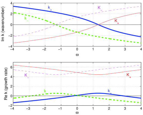
Figure 1: (color online) All four solutions of the dispersion relation for the pure FDO case with a Hopf unstable local system and no differential transport.  The two lower solutions are labelled $k_{\pm}$ and the two upper solutions are $K_{\pm}$.  $K_{+}$ and $k_{+}$ are both associated with the eigenvector $\mathbf{u}_{+}$ and the other two with $\mathbf{u}_{-}$.  

II.2 The effects of differential transport

With the pure FDO case as a comparison, we now examine the effects of differential transport and the convective, boundary driven manifestations of DIFI and Turing instabilities.    Typical results are shown in figs. 2-8 using the Fitzhugh-Nagumo-like FNModel (FN) model (10-11) for the local dynamics.

The key features of the relevant solutions in the FDO case are that $k_{+}$ has a growth peak and the associated phase velocity has a pole at positive $\omega$, while $k_{-}$ has a peak and pole on the opposite side, $\omega<0$.   A brief summary of the effects of differential transport on the dispersion relation solutions is as follows:

1. The primary effect of differential flow is to displace and distort the positive-$\omega$ peak of $k_{+\text{ }}$(and its mirror image in $k_{-}$).  Depending on the details of the model, the peak may be shifted to the left, right, upward or downward.  The pole in the phase velocity may also be shifted left or right.  If sufficiently strong,  differential flow can raise the peak growth rate from negative to positive, thus giving an instability even for a stable fixed point.  This is precisely what happens in DIFI.  For $\delta_{V}\neq 1$,  the peak growth rate may occur quite far from the pole of the phase velocity; thus the strongest instability is to a travelling wave solution rather than to a uniform oscillation.

2.  The most important effect of differential diffusion in the absence of differential flow ($\delta_{D}\neq 1,\delta_{v}=1$) is to alter the shape of the negative-$\omega$ tail of the $k_{+}$ solution (or, equivalently, the positive tail of $k_{-}$).  For fast inhibitor diffusion ($\delta_{D}<1$) the negative tail can develop first an inflection point and then a second growth rate peak.   The modes within this second peak are distinguished by the following features, confirming their interpretation as Turing patterns imposed by the boundary condition and advected with the flow:   A)  Their phase velocities are all very close to unity (in units where the flow velocity is 1) showing that they are stationary in the comoving frame.  B)  The amplitude ratio $R$ from the associated eigenvector is almost purely real, meaning that, contrary to the situation in self-sustained oscillations,  there is no phase lag between the two species (the activator and inhibitor are almost exactly in phase or $\pi$ out of phase).

For the most general case of differential transport, then, the dispersion relation has either one or two peaks, which we can identify as Hopf/FDO/DIFI and Turing peaks respectively.   Changing $\delta_{D}$ can alter the shape of the FDO peak and conversely, $\delta_{V}$ can alter the Turing peak, but they generally retain a separate identity, and for the most part exist in a “see-saw” relation.

We now illustrate these statements using examples based on particular models for the form of the Jacobian.  The examples we present in figures 2-8 and the nonlinear simulations used a form of the FitzHugh-Nagumo (FN) modelFNModel ,  for which the local dynamics is given by

$$\frac{dA}{dt} =\varepsilon(A-A^{3}-B)$$ (10)

$$\frac{dB}{dt} =-B+2A$$

and the Jacobian is

$$\mathbf{J=}\begin{pmatrix}\varepsilon&-\varepsilon\\ 2&-1\end{pmatrix}$$ (11)

where $\varepsilon$ is a control parameter.  $A$ and $B$ play the roles of activator and inhibitor, respectively.  A Hopf bifurcation occurs at $\varepsilon=1$;  the fixed point is unstable for $\varepsilon>1$.   We also studied another model using the simpler Jacobian

$$\mathbf{J}=\begin{pmatrix}\alpha&1\\ -1&\alpha\end{pmatrix}$$ (12)

with control parameter $\alpha$ and Hopf instability for $\alpha>0$,  hereafter referred to as the “$\alpha$-model.”  For the $\alpha$-model with $\alpha>0$, both species are autocatalytic, but one inhibits the other.  In most cases, qualitatively similar results were obtained for both models. When the results for the $\alpha$-model differ from theose of the FN model, we describe them verbally.

Figures 2 and 3 show typical effects of differential flow on the FDO peak.  Differential flow with either fast inhibitor or fast activator transport shifts the position and height of the peak growth rate.  It can also shift slightly the location of the pole in the phase velocity (i.e., the zero of $\operatorname{Im}k$)  but usually this shift is less pronounced than the shift of the peak in $\operatorname{Re}k$.  In the case shown in figures 2 and 3,  the peak height and location are both apparently monotonic in $\delta_{v}$ near $\delta_{v}=1$;  the peak shifts upward and to the right as $\delta_{v}$ decreases.   This is not universal, however.  In some cases (see for example figures 4 and 7 below),  the peak height has its minimum when $\delta_{v}=1$, so that faster flow of either species raises the height of the instability peak.  In one case we examined using the marginally stable $\alpha$-model with $\alpha=1$, the peak shifts to the right both for $\delta_{v}>1$ and $\delta_{v}<1$.   What has been referred to as the differential flow instability (DIFI)  can be understood a special case in which a growth rate peak whose maximum is less than zero in the absence of differential flow is shifted above zero when $\delta_{v}\neq 1$, thus creating a convective instability even though the fixed point of the local system is stable.  An example of this is shown in figure 4.  Physically, the shifting of the peak relative to the phase velocity pole means that in the presence of differential flow the fastest-growing mode is a travelling wave with some finite velocity, rather than a uniform oscillation.  From figure 3 it is evident that, while the amplitude ratio $R$ of the two species remains constant in the pure FDO case $\delta_{v}=1$,  differential flow modifies both their amplitude and phase relations in a frequency-dependent manner.

Figure 2: (color online) Effect of differential flow on the FDO peak.  FN model, $\varepsilon=1.5,D=0.1,\delta_{D}=1.$  $\delta_{v}=0.5,0.75,1,1.5,2.$ For the family of curves, the arrows show the direction of increasing $\delta_{v}$.  Dashed lines:  $\delta_{v}>1$; solid thin lines: $\delta_{v}<1$;  Thick line:  $\delta_{v}=1$.

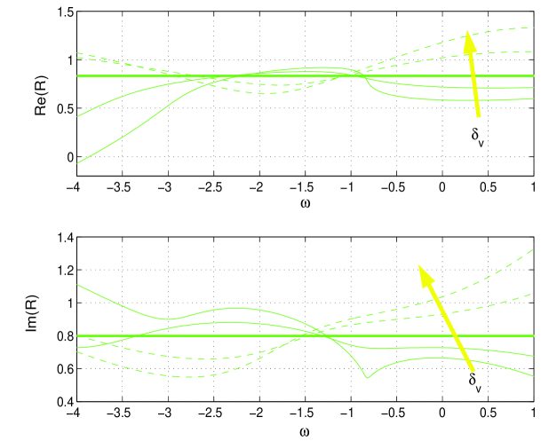
Figure 3: (color online) Amplitude ratios $R$ plotted for the same cases as in figure 2.  For the pure FDO case ($\delta_{v}=1$; thick line) the amplitude ratio is constant, corresponding to an eigenvector of the Jacobian.  In the presence of differential transport, however, it becomes frequncy-dependent.  The imaginary part of the amplitude ratio is related to the relative phase of the two components.  

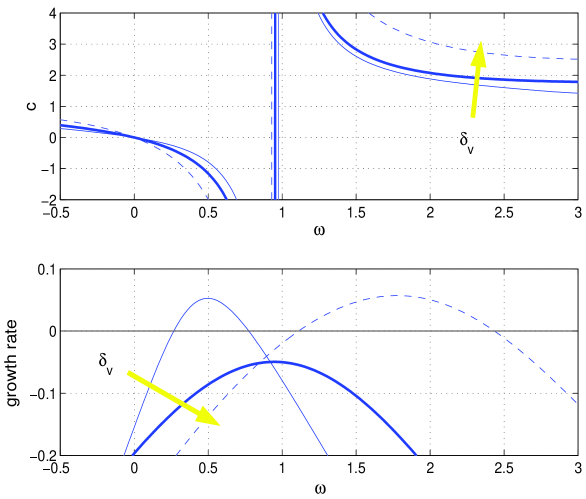
Figure 4: (color online) An example of the differential flow instability.  FN model, $\varepsilon=0.9$, $D=0.2$, $\delta_{D}=1$, $\delta_{v}=0.5$ (thin solid line), 1 (thick line), 2 (dashed line).  In the absence of differential flow,  there are no unstable modes, but there is nonetheless a peak in the (negative) growth rate at the natural oscillation frequency.  Sufficiently strong differential flow shifts the peak so that it rises above zero and unstable travelling wave modes appear.  For $\delta_{v}>1$, the unstable modes are downstream travelling waves, for $\delta_{v}<1$ they are upstream.  The medium remains stable against uniform oscillations.  Viewed in this way, the differential flow instability can be viewed as simply a continuous deformation of the FDO instability.  

Figures 5 and 6 show the effect of differential diffusion without differential flow $(\delta_{D}\neq 1,\delta_{v}=1)$.   A family of solution curves is shown for $\delta_{D}\leq 1$ (i.e., equal diffusion or fast inhibitor diffusion).  This is the case that renders a Turing instability possible in a stationary medium.  The growth rate peak is distorted somewhat relative to that of the pure FDO case.  This effect was more pronounced in some other examples we studied.  In one case, fast inhibitor diffusion lowered and broadened the FDO peak slightly while fast activator diffusion raised and sharpened the peak significantly.  In any case, however, the distortion of the FDO peak is rather less salient than the growth of a second peak at a different frequency.  When this second peak rises above zero, the modes contained within it have two important features:  First, their phase velocity is close to 1.  The phase velocity curves in fig. 5 flatten out at $c\approx 1$ for the range of amplified frequencies in the second peak.  This means that, in the co-moving frame, the waves are stationary.   Second, for frequencies within the range of the second peak,  the imaginary part of the amplitude ratio $\operatorname{Im}R$ is very small,  indicating a lack of phase lag between the two components.   Both of these observations are consistent with the Turing instability caused by differential diffusion.  Because diffusion is directionally symmetric, a mechanism driven by differential diffusion cannot cause a phase lag between the two components.  Turing patterns are reflection-symmetric, and stationary in the co-moving frame.  In view of these observations we attribute the second peak to Turing-like modes and refer to it as a Turing peak.  In this example it is quite clearly separated from the FDO peak,  the latter being characterized by strongly frequency dependent phase velocities and a non-zero, imaginary component $\operatorname{Im}R$ of the amplitude ratio.  There is a range of frequencies between the two peaks for which there are only damped modes.   In some cases, however, the two peaks can grow broader and almost merge, so that as the driving frequency changes, the resulting waves change continuously from an FDO-like to a Turing-like character.  Even in such cases, the Turing modes are distinguishable by means of their near-unity phase velocities and nearly real amplitude ratios.

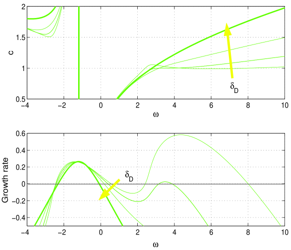
Figure 5: (color online) The effect of differential diffusion on the dispersion relation in the absence of differential flow.  FN model, $\varepsilon=1.5,D=0.2,\delta_{v}=1$.  $\delta_{D}=0.1,0.25,0.5,1.$  Thick line: $\delta_{D}=1$; thin lines: $\delta_{D}<1$.  Arrows show the direction of increasing $\delta_{D}$.  As $\delta_{D}$ decreases, the FDO peak is distorted slightly, but much more noticeable is the growth of a second peak.  The modes in this peak can be identified as Turing modes.  Their phase velocity is close to 1, and, as shown in fig 6, their amplitude ratio is almost purely real.  

Figure 6: (color online) Amplitude ratio $R$ plotted for the same cases as in figure 5.  The imaginary component nearly vanishes for frequencies within the Turing peak.  Near the FDO peak, on the other hand, the amplitude ratio is close to that of an eigenvector of the Jacobian.  

In figures 7 and 8, we examine the interaction between differential flow and differential diffusion, allowing both differential transport modes to operate simultaneously, as in refs. Satnoianu1 Satnoianu2 RazvanNew .  Here we plot the dispersion solutions for a constant value of $\delta_{D}$ as $\delta_{v}$ varies.  $\delta_{D}$ is such that a well-defined Turing peak exists for $\delta_{v}=1$.   We observe that setting $\delta_{v}\neq 1$ shifts the FDO peak as we expect.  In this case, unlike that of figure 2 but similar to fig. 4, the peak grows higher for either fast activator or fast inhibitor flow.  On the other hand,  the Turing peak is lowered for any $\delta_{v}\neq 1$.  The two peaks appear to have a “see-saw” relation.   Differential flow has other effects on the modes within the Turing peak.  Their velocity begins to depart from unity and is less uniform across the peak, and the amplitude ratio is no longer purely real.  In these senses,  the “Turing” modes begin to lose their Turing-like character in the presence of differential flow, even though one can still perceive two separate peaks in the growth rate.

Figure 7: (color online) Interacting effects of differential flow and diffusion.  Here the differential diffusion is constant, and the velocity ratio is varied.  FN model, $\varepsilon=1.2,D=0.05,\delta_{D}=0.15.$ $\delta_{v}=0.5,0.75,1,1.5,2.$  Thick curve: $\delta_{v}=1$; thin solid curves: $\delta_{v}<1$; dashed curves: $\delta_{v}>1$.  With increasing flow ratio, the two peaks are shifted closer together and begin to merge.  Departure from equal flow in either direction raises the height of the FDO peak while lowering the Turing peak.  Departure from equal flow also causes the phase velocities of the Turing modes to depart from 1.  

Figure 8: (color online) Amplitude ratios plotted for the same cases as in fig. 7

III Nonlinear Simulations

We now show the results of some nonlinear simulations of the FitzHugh-Nagumo flow system in order to illustrate the application of the dispersion relations to experiments. We choose to simulate the FN model with $\varepsilon=1.5$, $D=0.05$, $\delta_{v}=1$ and $\delta_{D}=0.2$.  As in the examples of figures 5 and 6, the dispersion relation shows both an FDO and a Turing peak.  The natural oscillation frequency (the pole in the phase velocity) is $\omega_{0}\approx 1.2$.   For comparison with the simulations, we plot both solutions $k_{\pm}$ on the same axes, for physical frequencies $\omega>0.$  These plots are shown in figs. 9-10.  Figure 11  shows a series of simulations with different driving frequencies.  The boundary conditions for these simulations were given by

$$\mathbf{u}(0,t)=a_{0}\begin{pmatrix}\cos\omega t\\ \sin\omega t\end{pmatrix}$$

where $a_{0}=0.05$.  The plots in the left column of this figure show the space-time patterns of the waves generated by the boundary perturbation.  The dotted white line in each plot represents the trajectory of a point co-moving with the flow. This allows the phase velocities of the waves to be compared readily with the flow velocity.  The plots in the right column show both dynamical variables $a$ and $b$ as functions of position for a single time. The latter plots allow an examination of the waveforms, including the phase shifts between activator and inhibitor.  The dispersion relation (fig. 9) predicts a positive growth rate at $\omega=0$, and, accordingly,  a constant (zero-frequency) perturbation indeed gives rise to growing stationary waves which saturate at a finite amplitude.   At $\omega=0.9$, below the natural frequency, the dispersion relation shows that both $k_{+}$ and $k_{-}$ have positive growth rates. $k_{-}$ (the solid curves in fig. 9) gives waves with a phase velocity of $\sim 0.5$, i.e.,  downstream waves moving slower than the flow velocity, while $k_{+}$ gives waves with a negative phase velocity, i.e., upstream travelling waves.   Near the boundary,  a superposition of both waves occurs, but the upstream waves have a much larger growth rate and they dominate at positions farther downstream, crowding out the other mode entirely and reaching a nonlinear saturated amplitude.  At $\omega=2.5>\omega_{0}$,  only $k_{+}$ has a positive growth rate, giving waves with an positive (downstream) phase velocity faster than the flow speed.  A small admixture of the other mode $k_{-}$ can be discerned near the boundary, but it decays rapidly with downstream distance.   $\omega=3.5$ falls within the gap between the FDO and Turing peaks.  Thus there are no growing modes at this frequency and the disturbance decreases with downstream distance.   $\omega=5$, however, lies within the Turing peak of the $k_{-}$ solution.  As predicted by the dispersion relation, the resulting waves have a velocity nearly equal to the flow velocity and there is almost no phase difference between the two species.

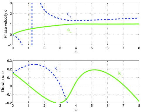
Figure 9: (color online) Growth rate and phase velocity as functions of frequency for the model of our nonlinear simulations.  Both relevant solutions are plotted

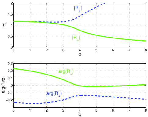
Figure 10: (color online) Modulus and phase of the complex amplitude ratio.  The modulus gives the ratio of the peak amplitudes for the oscillations of the two dynamical variables, while the phase gives the relative phase shift.  

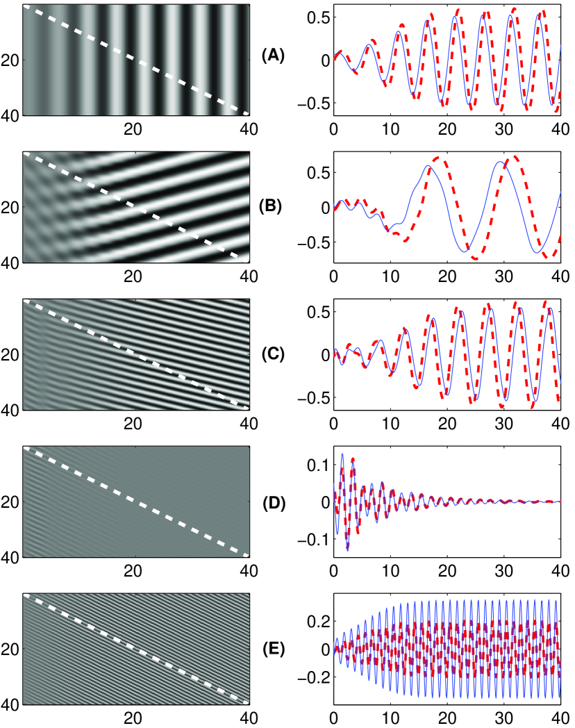
Figure 11: (color online):  Results of nonlinear simulations of the FN model for sinusoidal boundary perturbations at five different frequencies.  a) 0 b) 0.9 c) 2.5 d) 3.5  e) 5.   Left column:  space(horizontal) vs. time (vertical) plots with gray scale whowing concentration $A.$ Right column:  concentrations $A$ (thin line), $B$ (thick dashed line) vs. space (horizontal axis).  

The amplitude and phase characteristics of the nonlinear waveforms may also be compared with the predictions of the linear dispersion relation, and in this case the agreement is quite close.  In the complex exponential solution eq. 3,  the modulus of the ratio $R=v/u$ gives the ratio of the peak amplitudes of the oscillations of the two dynamical variables, while the argument of $R$ gives the relative phase.  For frequencies within the FDO peak,  our nonlinear simulations show that, as one expects from figure 10, the ratio of the peak amplitudes of $b$ and $a$ is slightly larger than unity, while the phase shift is approximately $\pi/4$.  For $\omega=5$,  on the other hand, the linear dispersion relation gives a very small phase shift for the relevant $k_{-}$ solution, and an amplitude ratio slightly larger than $0.5$.  The phase shift is indeed almost zero and the $b$ amplitude is indeed smaller than that of $a$.  The actual amplitude ratio in the saturated waveform is approximately $0.6$, close to the prediction of the linearized analysis.

Finally, we note that at frequencies where more than one mode is present, one can be selected by manipulating the driving function itself so as to align it with one eigenvector or the other.  As an example, consider $\omega=0.9$, a frequency at which both solution branches exhibit positive growth rates.  Here, we find that for the faster-growing $k_{+}$ mode the complex amplitude ratio is $R_{+}\approx 0.84-0.8i$ while for the other mode $R_{-}\approx 0.94+0.68i$.  The driving function used in fig. 11 excites both of these modes and a superposition is seen near the upstream boundary.  By tuning the driving function to be

$$\mathbf{u}(0,t)=a_{0}\operatorname{Re}\begin{pmatrix}1\\ R_{+}\end{pmatrix}e^{i\omega t}=a_{0}\operatorname{Re}\begin{pmatrix}e^{i\omega t}\\ \left|R_{+}\right|e^{i(\omega t+\phi_{+})}\end{pmatrix}=a_{0}\begin{pmatrix}\cos\omega t\\ 0.84\cos\omega t+0.8\sin\omega t\end{pmatrix},$$

however,  we can excite mostly the $k_{+}$ mode so that the upstream travelling waves appear almost uncontaminated.  Conversely, by choosing the amplitude and phase of the driving to align with the other eigenvector, we excite mostly the other, $k_{-}$ mode.  Eventually, however, the other, faster-growing mode begins to appear, possibly through nonlinear effects or through the small admixture still present in the boundary condition,  and the $k_{+}$ mode eventually wins in the asymptotic downstream region.  Simulation results which show this selection effect are plotted in figure 12.

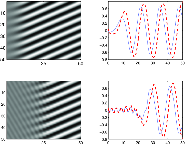
Figure 12: (color online) Simulations with sinusoidal boundary perturbations at $\omega=0.9$, but with the driving amplitudes and phases tuned to select the upstream (top) or downstream (bottom) mode.  Even if the downstream mode is selected near the boundary, the faster-growing upstream mode eventually takes over farther downstream.  As in fig. 11, the plots on the left are space-time, and those on the right are of $A$ and $B$ vs. position.  

IV Conclusions and experimental tests

We have examined the linear stability analysis relevant to the convective growth of spatiotemporal patterns in a reactive flow system, excited by a small sinusoidal perturbation of a fixed point at the inflow boundary. We examined the real and imaginary parts of the wavenumber as functions of the real boundary forcing frequency. They represent the downstream growth rate and periodicity of the disturbances caused by a boundary perturbation.  We found that the growth rate as a function of frequency exhibits at most two physically distinct peaks corresponding to two types of waves, one or both of which may be present and convectively unstable. We found that, in addition to the phase velocity, the complex ratio $R$ of activator and inhibitor concentrations, which encodes the relative amplitude and phase of oscillations in the activator and inhibitor concentrations, provides an additional criterion for distinguishing the types of modes.  Turing-like modes are distinguished from FDO-like modes by the lack of a phase lag between the two components and by phase velocities that are close to the flow velocity, so that in the co-moving frame they are stationary patterns. Viewing the different types of modes as belonging to peaks in the growth rate, we saw the close relationship between FDO and the differential flow instability.  One can be viewed as a continuous deformation of the other.  A primary effect of differential flow is to shift the FDO peak.  What has been referred to as the differential flow instability (the appearance of a travelling wave instability in a medium which is neither Hopf nor Turing unstable) can be interpreted as a case in which a sub-threshold FDO peak is shifted sufficiently to bring it above zero and to create unstable modes (fig. 4).

We now comment on experimental verifications of the present predictions. The presence of two peaks could be seen in an experiment in which the perturbation frequency at the inflow is the control parameter.  Frequencies for which the growth rate is positive will result in sustained waves, while the waves will die out and fail to propagate if the growth rate is negative.  Based on our results we expect that growing waves will appear within at most two frequency ranges.  The phase velocities can also be measured and compared with our general findings.

Two types of experiments may be envisaged, in which oscillatory driving is implemented differently.  The first type Kaern6 Miguez1 Santiago makes use of a linearly growing, light-sensitive reaction-diffusion system.  The effective moving boundary is provided by a moving mask which extinguishes the reaction on the illuminated side of a moving line.   The illumination at the moving boundary can be modulated periodically, resulting in an oscillatory perturbation. In these experiments, differential diffusion $\delta_{D}\neq 1$ is achieved by immobilizing one species on a gel, but differential flow is absent, $\delta_{v}=1$.

The second type of experiment is conducted in a packed bed reactor (PBR), which is by the outlet of a continuous stirred tank reactor (CSTR).Kaern1 Bamforth3 Toth Kaern2 Kaern5 Rovinsky93  The CSTR may be manipulated to be stationary or to oscillate slower or faster than the medium in the PBR. This leads to stationary, upstream and downstream moving waves Kaern1 Kaern3 Kaern4 Kaern5 Faraday . By packing the PBR with ion-exchanger beads that immobilize either activator or inhibitor, conditions of simultaneous differential diffusion and differential flow may be obtained.  Refs. Satnoianu1 Satnoianu2  modelled this by setting $\delta_{D}=\delta_{v}.$  It is a challenge to devise experiments in which the flow ratio, diffusion ratio and driving frequency can be varied independently. While the phase velocities of travelling waves can easily be measured,  verification of other properties of the waves may present experimental challenges. Verification of the predicted phase relationships would require simultaneous measurements of both activator and inhibitor concentrations.

References

- (1) P. Andrésen, M. Bache, E. Mosekilde, G. Dewel and P. Borckmans, Phys. Rev. E. 60, 297 (1999).
- (2) S.P. Kuznetsov, E. Mosekilde, G. Dewel, and P. Borckmanns, J Chem. Phys. 106, 7609 (1997).
- (3) J.R. Bamforth, S. Kalliadasis, J. H. Merkin, S. K. Scott, Phys. Chem. Chem. Phys. 2, 4013 (2000).
- (4) J.R. Bamforth, J. H. Merkin, S.K. Scott., R.Toth and V. Gaspar, Phys. Chem. Chem. Phys. 3, 1435 (2001).
- (5) M. Kærn and M. Menzinger. Phys. Rev. E. 60, 3471 (1999); 62, 2994 (2000); P. Andresen, E. Mosekilde, G. Dewel and P. Borckmans, Phys. Rev. E 62, 2992 (2000).
- (6) M. Kærn, M. Menzinger, A. Hunding, Biophys. Chem. 87, 121 (2000).
- (7) M. Kærn, M. Menzinger, A. Hunding, J. Theor Biol. 207, 473 (2000).
- (8) M. Kærn, M. Menzinger, R. Satnoianu and A. Hunding, Faraday Disc. 120, 295 (2002).
- (9) A.B. Rovinsky and M. Menzinger, Phys.Rev.Let. 69, 1193 (1992).
- (10) X.G.Wu, S.Nakata, M.Menzinger and A.Rovinsky, J.Phys.Chem. 100, 15810-15814 (1996).
- (11) R. Satnoianu and M. Menzinger, Phys. Rev. E. 62, 113 (2000).
- (12) R. Satnoianu, P.K. Maini and M. Menzinger., Physica D 160, 79, (2001).
- (13) R. Satnoianu, Phys. Rev. E 68, 032101 (2003).
- (14) P. McGraw and M. Menzinger, Phys.Rev. E 62 066122 (2003).
- (15) Vasquez D., Phys. Rev. Let., in press.
- (16) J.R. Bamforth, R. Toth, V. Gaspar and S.K. Scott, Phys. Chem. Chem. Phys. 4, 1299 (2002).
- (17) R. Toth, A. Papp, V. Gaspar, J.H. Merkin, S.K. Scott and A.F. Taylor, Phys. Chem. Chem. Phys. 3, 957 (2001).
- (18) M. Kærn, M. Menzinger. Phys. Rev. E. 61, 3334 (2000).
- (19) M. Kærn and M. Menzinger M., J. Phys. Chem. 106, 4897 (2002).
- (20) M. Kaern, D.G. Miguez, A. P. Munuzuri and M. Menzinger, Biophys. Chem. 110, 231 (2004).
- (21) A.B. Rovinsky and M. Menzinger, Phys.Rev.Let. 70, 778 (1993).
- (22) M. Kaern, R. Satnoianu, A. Munuzuri and M. Menzinger, Phys. Chem. Chem. Phys. 4, 1315 (2002).
- (23) A.M. Turing, Philos. Trans. R. Soc. London, Ser. B 237, 37 (1952).
- (24) R. Kapral R. and K. Showalter, Chemical waves and patterns. (Kluwer, Dorderecht,1995).
- (25) M. Menzinger and A.B. Rovinsky, “The Differential Flow Instability,” in R. Kapral and K. Showalter, Chemical waves and patterns. (Kluwer, Dorderecht,1995).
- (26) M.R.E. Proctor, S.M. Tobias and E. Knobloch, Physica D 145, 191 (2000).
- (27) R.J. Deissler, J. Stat. Phys. 40, 371 (1985); 54, 1459 (1989).
- (28) Wolpert L., Principles of Development. (Oxford Univ. Press, 1998).
- (29) J.D. Murray, Mathematical Biology II: Spatial models and biomedical applications. (Springer, Berlin, 2003)
- (30) C.B. Muratov and V.V. Osipov, Phys. Rev. E 54, 4860 (1996). S.P. Dawson, M.V. D’Angelo and J.E. Pearson, Phys. Lett. A 265, 346 (2000). A. Hagberg and E. Meron, Chaos 4, 477 (1994).
- (31) D.G. Miguez, R. Satnoianu, A.P. Munuzuri. Submitted to Phys. Rev. Lett.