Elliptic instability in the Lagrangian-averaged Euler-Boussinesq-alpha equations

Abstract

We examine the effects of turbulence on elliptic instability of rotating stratified incompressible flows, in the context of the Lagrangian-averaged Euler-Boussinesq-alpha, or LAEB$-\alpha$, model of turbulence. We find that the LAEB$-\alpha$ model alters the instability in a variety of ways for fixed Rossby number and Brunt-Väisälä frequency. First, it alters the location of the instability domains in the $(\gamma,\cos\theta)-$parameter plane, where $\theta$ is the angle of incidence the Kelvin wave makes with the axis of rotation and $\gamma$ is the eccentricity of the elliptic flow, as well as the size of the associated Lyapunov exponent. Second, the model shrinks the width of one instability band while simultaneously increasing another. Third, the model introduces bands of unstable eccentric flows when the Kelvin wave is two-dimensional. We introduce two similarity variables–one is a ratio of the Brunt-Väisälä frequency to the model parameter $\Upsilon_{0}=1+\alpha^{2}\beta^{2}$, and the other is the ratio of the adjusted inverse Rossby number to the same model parameter. Here, $\alpha$ is the turbulence correlation length, and $\beta$ is the Kelvin wave number. We show that by adjusting the Rossby number and Brunt-Väisälä frequency so that the similarity variables remain constant for a given value of $\Upsilon_{0}$, turbulence has little effect on elliptic instability for small eccentricities $(|\gamma|\ll 1)$. For moderate and large eccentricities, however, we see drastic changes of the unstable Arnold tongues due to the LAEB$-\alpha$ model. Additionally, we find that introducing anisotropy in the vertical component of the transported velocity field merely alters the definition of the model parameter $\Upsilon_{0}$, which effectively reduces the original parameter value. When the similarity variables are viewed with the new definition, the results are similar to those for the isotropic case.

I Introduction

This paper is the third in a continuing investigation of the effects of a turbulence closure model on the classic solution of elliptic instability. The first fab:holm:03 examined the effects of the Lagrangian-averaged Navier-Stokes-alpha, or LANS$-\alpha$, turbulence closure model in an inertial frame. The second fab:holm:04a examined the effects of this turbulence model in a rotating frame, as well as the effects of a few related turbulence closure models. In the present paper, we continue the investigation by examining the effect of stratification with rotation in the inviscid LANS$-\alpha$ model, also called the Lagrangian-averaged Euler-Boussinesq-alpha, or LAEB$-\alpha$, model holm:marsden:rat:98a ; holm:99 ; holm:mar:rat:02 .

Turbulence models are ubiquitous in fluid mechanics today. They are used with the hopes that they adequately describe the evolution of real-world flows, governed by the Navier-Stokes equations. The question that arises, then, is how do individual turbulence models affect classical solutions of the Navier-Stokes equations? A natural thought process is that a model which preserves classical solutions is preferred over a model which drastically alters the solutions. However, imposing such a strict requirement on a turbulence model is unrealistic. An alternative thought process asks how to change the problem so that the effects of the model on classical solutions is negated while using the low-resolution advantage the turbulence model possesses. Our present investigation has two goals. First, we seek to understand how the LAEB$-\alpha$ turbulence model affects the classical solution known as elliptic instability. The model is formulated in a way that preserves the existence of the solution, something which is not possible with every turbulence model. We find that the model alters the instability, which leads to our second goal. Namely, we seek a reformulation of the problem so that the effects are negated. Turbulence models are being used in applications such as ocean circulation. Our motivation is to determine how turbulence closure models affect instabilities before implementing the models in such applications.

The LAEB$-\alpha$ model is a turbulence closure model which has two velocities, a transport velocity and a transported velocity. The transport velocity $\mathbf{u}$ is smoother that the velocity $\mathbf{v}$ (or momentum) which it transports, given by the relation $\mathbf{v}=(1-\alpha^{2}\Delta)\mathbf{u}$ in the isotropic version. (An anisotropic version will be given in Section 5.) This approach was first introduced by Leray leray:34 as a regularization of the Navier-Stokes equations. Here, the parameter $\alpha$ is interpreted as the turbulence correlation length. The idea is that in numerical simulation, $\alpha$ is set to be the grid size, and that the dynamics which occur at scales smaller than $\alpha$ are swept along to scales larger than $\alpha$ by the transport velocity $\mathbf{u}$.

Elliptic instability is a mechanism by which two-dimensional swirling flows become unstable to three-dimensional perturbations. The instability in the Euler equations was investigated by Lord Kelvin kelvin for the case of circular streamlines and by Bayly bayly:86 for elliptic streamlines. Further work by others craik:crim:86 ; craik:88 ; craik:89 ; wal:90 ; miya:fuku:92 ; kers:93 ; miya:93 ; leb:03 examined the effects of rotation, stratification, and magnetic fields on the instability. We refer the reader to a recent reviewkers:02 for details about the history of elliptic instability. It is a member of the Craik-Criminale, or CC, class of exact solutions to the Navier-Stokes equations craik:crim:86 . The velocity field in this class of solutions is the sum of a flow linear in the spatial coordinates and a Kelvin wave. The present authors have shown that this class of solutions are valid in a family of turbulence closure models fab:holm:04a . This investigation is continued here.

The paper is organized as follows. In Section 2, we state the LAEB$-\alpha$ equations and discuss the CC class of solutions for these equations. We examine a specific member of this class in Section 3, namely elliptic instability. We combine analysis and numerical simulation to give a full description of elliptic instability in the isotropic LAEB$-\alpha$ model in Section 4. The analysis yields two similarity variables which fully describe the behavior of the instability for elliptic flows of small eccentricity. We briefly discuss the effects of the anisotropic version of the LAEB$-\alpha$ model in Section 5. We show that the effects of anisotropy are similar to the isotropic version, once the similarity variables of Section 4 are redefined. Finally, Section 6 concludes the paper with a summary of our findings, including a conjecture as to why the model alters the unstable Arnold tongues for moderate and large eccentricities.

II CC solutions in LAEB$-\alpha$ equations

The isotropic version of the LAEB$-\alpha$ equations holm:marsden:rat:98a ; holm:99 ; holm:mar:rat:02 are

$$\partial_{t}\mathbf{v}+\mathbf{u}\cdot\nabla\mathbf{v}+(\nabla\mathbf{u})^{T}\cdot\mathbf{v}+2\mathbf{\Omega}\times\mathbf{u}+bg\mathbf{e}_{z}+\nabla\left(p-\frac{1}{2}|\mathbf{u}|^{2}-\frac{\alpha^{2}}{2}|\nabla\mathbf{u}|^{2}\right)=\mathbf{F},$$ (1)

$$\partial_{t}b+\mathbf{u}\cdot\nabla b=0,$$ (2)

$$\text{div}\,\mathbf{u}=0.$$ (3)

The variables are as follows:

• $\mathbf{v}=(1-\alpha^{2}\Delta)\mathbf{u}$ is the fluid velocity field,

• $\mathbf{u}$ is the mean transport fluid velocity field,

• $p$ is the pressure,

• $b=b(z)$ is the dimensionless buoyancy term which reflects the deviation from mean density [that is, we have taken $\rho=\rho_{0}(1+b)$],

• $\mathbf{\Omega}=\Omega\mathbf{e}_{z}$ is the Coriolis force,

• $g$ is the gravitational constant,

• $\mathbf{F}$ is the contribution of all external body forces,

• in index notation, $(\nabla\mathbf{u})_{ij}=\partial_{j}u_{i}=u_{i,j}$.

The equations reduce to the classic Euler-Boussinesq (EB) equations upon setting $\alpha=0$. The equations admit solutions $(\mathbf{u},p,b)=(\mathbf{U}_{0},P_{0},b_{0})$ given by $\mathbf{U}_{0}=\mathcal{S}(t)\cdot\mathbf{x}+\bar{\mathbf{U}}(t)$, $P_{0}=\mathbf{x}^{T}\cdot\mathcal{T}(t)\cdot\mathbf{x}+P(t)$, and $b_{0}(z)=s(h-z)$, provided

$$d_{t}\mathcal{S}_{ij}+\mathcal{S}_{ir}\mathcal{S}_{rj}+2\Omega\epsilon_{i3p}\mathcal{S}_{pj}-sg\delta_{3i}\delta_{3j}=\mathcal{M}_{ij},$$ (4)

$$\mathcal{S}_{ii}=0,$$ (5)

where we sum over repeated indices. Here, $\mathbf{V}_{0}=(1-\alpha^{2}\Delta)\mathbf{U}_{0}=\mathbf{U}_{0}$, and the (symmetric) Hessian $\mathcal{M}$ is defined by $\mathcal{M}_{ij}=-\partial_{i}\partial_{j}\mathbb{P}$, where

$$\mathbb{P}=p-\int\mathbf{F}\cdot\,d\mathbf{x}+(d_{t}\bar{U}_{q}-\mathcal{S}_{qr}\bar{U}_{r}+shg\delta_{3q})x_{q}\,.$$

The Brunt-Väisälä frequency, defined for the EB equations as $N^{2}=-(g/\rho_{0})(d\rho/dz)$, is $N^{2}=sg$ with $s>0$.

One can construct a new exact solution of the LAEB$-\alpha$ equations of the form

$$\mathbf{u}=\mathbf{U}_{0}+\mathbf{U}_{1},\quad b=b_{0}+b_{1},\quad p=P_{0}+P_{1}.$$ (6)

Consequently, $\mathbf{v}=\mathbf{V}_{0}+\mathbf{V}_{1}$, where $\mathbf{V}_{1}=(1-\alpha^{2}\Delta)\mathbf{U}_{1}$. The generic equations of motion for $\mathbf{V}_{1}$, $b_{1}$, and $P_{1}$ are

$$\begin{split}&\partial_{t}\mathbf{V}_{1}+\mathbf{U}_{0}\cdot\nabla\mathbf{V}_{1}+\mathbf{U}_{1}\cdot\nabla\mathbf{V}_{0}+\mathbf{U}_{1}\cdot\nabla\mathbf{V}_{1}+(\nabla\mathbf{U}_{0})^{T}\cdot\mathbf{V}_{1}+(\nabla\mathbf{U}_{1})^{T}\cdot\mathbf{V}_{0}\\ &\hskip 20.00003pt+(\nabla\mathbf{U}_{1})^{T}\cdot\mathbf{V}_{1}+2\mathbf{\Omega}\times\mathbf{U}_{1}+b_{1}g\mathbf{e}_{z}-(\nabla\mathbf{U}_{0})^{T}\cdot\mathbf{U}_{1}-(\nabla\mathbf{U}_{1})^{T}\cdot\mathbf{U}_{0}\\ &\hskip 20.00003pt+\nabla\left(P_{1}-\frac{1}{2}|\mathbf{U}_{1}|^{2}-\frac{\alpha^{2}}{2}|\nabla\mathbf{U}_{1}|^{2}-\alpha^{2}(\nabla\mathbf{U}_{0})_{ij}(\nabla\mathbf{U}_{1})_{ij}\right)=\mathbf{0},\end{split}$$ (7)

$$\partial_{t}b_{1}+\mathbf{U}_{0}\cdot\nabla b_{1}+\mathbf{U}_{1}\cdot\nabla b_{0}+\mathbf{U}_{1}\cdot\nabla b_{1}=0,$$ (8)

$$\text{div}\,\mathbf{U}_{1}=0.$$ (9)

Equations (7) and (8) contain two nonlinear terms. We choose the disturbance for the buoyancy and transport velocity field $\mathbf{u}$ in the form of a traveling Kelvin wave:

$$\mathbf{U}_{1}=\mu\mathbf{a}(t)e^{i\beta\psi},\quad b_{1}=s\mu\hat{b}(t)e^{i\beta\psi},\qquad P_{1}=\mu\hat{p}_{1}(t)e^{i\beta\psi}+\mu^{2}\hat{p}_{2}(t)e^{2i\beta\psi},$$ (10)

where $\psi(\mathbf{x},t)=\mathbf{k}^{T}(t)\cdot\mathbf{x}+\delta(t)$, $\beta$ is the wave number chosen so that $|\mathbf{k}(0)|=1$, and $\mu$ is a scaling parameter so that $|\mathbf{a}(0)|=1$. Consequently, the transported velocity field has the form $\mathbf{V}_{1}=\mu\Upsilon(t)\mathbf{a}(t)e^{i\beta\psi}$, where

$$\Upsilon(t)=1+\alpha^{2}\beta^{2}|\mathbf{k}(t)|^{2}.$$ (11)

We refer to solutions of the form (6) with (10) as Craik-Criminale, or CC, solutions craik:crim:86 . A CC solution can be viewed as the sum of a ‘base flow’ $\mathbf{U}_{0}$ plus a ‘disturbance’ $\mathbf{U}_{1}$ in the form of a traveling Kelvin wave. The incompressibility condition (9) yields transversality of the wave

$$\mathbf{k}^{T}\cdot\mathbf{a}=0.$$ (12)

Upon inserting (10) into (7) and (8), the terms in (7) and (8) nonlinear in the disturbance identically vanish due to wave transversality, implied by (12). The remaining terms are linear and constant in $\mathbf{x}$. The CC solution ansatz requires that the coefficients of these terms vanish separately, thereby yielding the following system of equations for the wave vector $\mathbf{k}$, wave amplitude $\mathbf{a}$, and pressure harmonics $\hat{p}_{1,2}$:

$$d_{t}\mathbf{k}^{T}\cdot\mathbf{x}+\mathbf{k}^{T}\cdot\mathcal{S}\cdot\mathbf{x}=0,$$ (13)

$$\begin{split}&d_{t}(\Upsilon\mathbf{a})+i\beta\Upsilon\mathbf{a}(d_{t}\delta+\mathbf{k}^{T}\cdot\bar{\mathbf{U}})+\mathcal{S}^{T}\cdot(\Upsilon\mathbf{a})+\mathbf{\Pi}\times\mathbf{a}-(i\beta\hat{p}_{1}-\alpha^{2}\beta^{2}\mathbf{k}^{T}\cdot\mathcal{S}\cdot\mathbf{a})\mathbf{k}\\ &\hskip 10.00002pt+N^{2}\hat{b}\mathbf{e}_{z}=\mathbf{0},\end{split}$$ (14)

$$sd_{t}\hat{b}+is\beta\hat{b}(d_{t}\delta+\mathbf{k}^{T}\cdot\bar{\mathbf{U}})+(\nabla b_{0})\cdot\mathbf{a}=0,$$ (15)

$$\hat{p}_{2}+(\Upsilon-1)|\mathbf{a}|^{2}=0.$$ (16)

Here, $\mathbf{\Pi}=2\mathbf{\Omega}+\text{curl}~{}\mathbf{U}_{0}$ is the total vorticity of the rotating coordinate system and the base flow. Without loss of generality, we set $d_{t}\delta+\mathbf{k}^{T}\cdot\bar{\mathbf{U}}=0$. We take the gradient of (13) and obtain the following system of equations:

$$d_{t}\mathbf{k}+\mathcal{S}^{T}\cdot\mathbf{k}=\mathbf{0},$$ (17)

$$d_{t}(\Upsilon\mathbf{a})+\mathcal{S}^{T}\cdot(\Upsilon\mathbf{a})+\mathbf{\Pi}\times\mathbf{a}-\tilde{P}\mathbf{k}+N^{2}\hat{b}\mathbf{e}_{z}=\mathbf{0},$$ (18)

$$d_{t}\hat{b}-\mathbf{a}\cdot\mathbf{e}_{z}=0,$$ (19)

subject to (12). The term $\tilde{P}$ represents the coefficient of $\mathbf{k}$ in (14). At this point, one may assume that $\mathbf{a}(t)$, $\hat{b}(t)$, $i\hat{p}_{1}(t)$, and $\hat{p}_{2}(t)$ are real-valued functions.

The operator $(d_{t}+\mathcal{S}^{T}\cdot)$ in (17) and (18) is the total derivative of a vector field in a Galilean frame moving with $\mathbf{U}_{0}$. Thus, these equations state that the wave vector $\mathbf{k}$ is frozen in the fluid, and the scaled amplitude $\Upsilon\mathbf{a}$ in the Galilean frame moving with $\mathbf{U}_{0}$ is affected by the total vorticity of the system, by pressure, by the buoyancy, and by the base flow. Once the CC solutions are established, introduction of the factors of $\Upsilon$ in equations (16) and (18) reveals the key differences between the elliptic instability analyses for the EB equations and the mean turbulence equations of the LAEB$-\alpha$ model.

As is common when working with incompressible fluids, the pressure term can be removed from the problem by taking the dot product of (18) with $\mathbf{k}$ and using the fact that $\mathbf{k}^{T}\cdot\mathbf{a}$ is an integral of motion:

$$\tilde{P}=\frac{\mathbf{k}^{T}\cdot(\Upsilon(\mathcal{S}+\mathcal{S}^{T})\cdot\mathbf{a}+\mathbf{\Pi}\times\mathbf{a}+N^{2}\hat{b}\mathbf{e}_{z})}{|\mathbf{k}|^{2}}.$$

Once (17) is solved for $\mathbf{k}$, the equations for $\mathbf{a}$ and $\hat{b}$ can be written compactly as

$$\frac{d}{dt}\begin{pmatrix}\mathbf{a}\\ \hat{b}\end{pmatrix}=\mathcal{N}(t;\ldots)\begin{pmatrix}\mathbf{a}\\ \hat{b}\end{pmatrix}.$$ (20)

Here, $\mathcal{N}$ is a $4\times 4$ matrix whose coefficients contain elements from $\mathcal{S}$ and $\mathbf{k}$, and the dots indicate parameter dependence.

Multi-harmonic disturbances.

Finally, we point out that for the EB equations (corresponding to $\alpha=0$), the perturbation can be over a sum of harmonics of $e^{i\beta\psi}$. In this case, different harmonics do not interact. This phenomenon changes slightly for the LAEB$-\alpha$ equations. For example, if we were to consider $\mathbf{U}_{1}=\mu\mathbf{a}^{(1)}\exp(i\beta\psi)+\mu^{2}\mathbf{a}^{(2)}\exp(2i\beta\psi)$ and similarly for $\mathbf{V}_{1}$ and $b_{1}$, then the correct form for the pressure perturbation $P_{1}$ would carry the first four harmonics of $\exp(i\beta\psi)$. The pressure coefficients $\hat{p}_{i}(t)$ of the first, third and four harmonics would be purely real. However, the coefficient of the second harmonic would be complex-valued such that the real part balances a contribution from $\mathbf{a}^{(1)}$ and the imaginary part from $\mathbf{a}^{(2)}$. Thus, different harmonics do interact, but the interaction is absorbed by the pressure. The remainder of the paper considers only single-harmonic disturbances.

III Elliptic instability

The classic problem of elliptic instability resides among the CC solutions. The base flow for elliptic instability is

$$\mathcal{S}=\bar{\omega}\begin{pmatrix}0&-1+\gamma&0\\ 1+\gamma&0&0\\ 0&0&0\end{pmatrix},\qquad\bar{\mathbf{U}}=\mathbf{0}.$$ (21)

This base flow is a rigidly rotating column of fluid whose streamlines are ellipses with eccentriticy $\gamma$ and vorticity $2\bar{\omega}\mathbf{e}_{z}$. We rescale time by $\bar{\omega}$ so that the Coriolis parameter $\Omega$ is replaced by $\Omega^{\prime}=\Omega/\bar{\omega}$, which we interpret as an inverse Rossby number miya:fuku:92 ; fab:holm:04a . We now suppress the prime notation. The extreme values of the solution in (21) represent pure shear at $\gamma=\pm 1$ (along different axes) and rigid body rotation at $\gamma=0$. The solution of (17) is

$$\mathbf{k}=\begin{pmatrix}\sin\theta\cos\hat{t}\\ \kappa\sin\theta\sin\hat{t}\\ \cos\theta\end{pmatrix},$$ (22)

where $\hat{t}=t\sqrt{1-\gamma^{2}}$, $\kappa^{2}=(1-\gamma)/(1+\gamma)$, and $\theta$ is the polar angle the wave vector $\mathbf{k}$ makes with the axis of rotation $\mathbf{e}_{z}$. We note that a more arbitrary initial orientation of $\mathbf{k}$ is equivilaent to a shift in the starting time $t\to t-t_{0}$.

In general, the solution of (20) must be simulated numerically. Since the coefficient matrix $\mathcal{N}$ in (20) is periodic with period $\tau=2\pi/\sqrt{1-\gamma^{2}}$, it follows that (20) can be rewritten as a pair of Schrödinger equations with periodic potentials, shown in the appendix. Thus, we analyze the system using Floquet theory yaku:star:76 . One needs to determine the eigenvalues $\rho_{i}$ of the monodromy matrix $\mathcal{P}(\tau)$, where $d_{t}\mathcal{P}=\mathcal{N}\cdot\mathcal{P}$ with the initial condition $\mathcal{P}(0)=\mathcal{I}_{4}=\text{diag}\{1,1,1,1\}$. The Lyapunov growth rates, which exist only if $\max_{i}|\rho_{i}|>1$, are given by $\sigma=\ln(\max_{i}|\Re(\rho_{i})|)/\tau$.

IV Isotropic LAEB$-\alpha$ model

We begin by examining the isotropic model presented in Section II. The classical results for the EB equations were obtained by Miyazaki and Fukumotomiya:fuku:92 and Miyazakimiya:93 . Rather than review the classical results separately, we will study the solution in the isotropic LAEB$-\alpha$ model directly, regaining the classical results upon setting $\alpha=0$, which is equivalent to setting $\Upsilon(t)\equiv 1$. To illustrate the effects of the model, we plot the classical results next to those generated by the model. The pièce de résistance of the present paper is the introduction of the similarity variables

$$\chi=\frac{N^{2}}{\Upsilon_{0}},\qquad\zeta=\frac{2|\Omega+1|}{\Upsilon_{0}},$$ (23)

where

$$\Upsilon_{0}=1+\alpha^{2}\beta^{2}.$$ (24)

Since $\alpha$ has dimensions of length, it follows that $\Upsilon_{0}$ is a dimensionless parameter.

IV.1 Circular streamlines–exact solutions

The circular case $\gamma=0$ can be analyzed analytically. Here, $|\mathbf{k}(t)|=1$, and any solution to (20) can be written as

$$\begin{pmatrix}\mathbf{a}\\ \hat{b}\end{pmatrix}=c_{1}\begin{pmatrix}\mathbf{a}_{1}\\ \hat{b}_{1}\end{pmatrix}+c_{2}\begin{pmatrix}\mathbf{a}_{2}\\ \hat{b}_{2}\end{pmatrix}+c_{3}\begin{pmatrix}\mathbf{a}_{3}\\ \hat{b}_{3}\end{pmatrix}+c_{4}\begin{pmatrix}\mathbf{a}_{4}\\ \hat{b}_{4}\end{pmatrix},$$ (25)

where

$$\mathbf{a}_{1} =\sin(\omega t+\phi)\mathbf{k}_{\perp 1}+\frac{1}{\sqrt{1+q^{2}\chi}}\cos(\omega t+\phi)\mathbf{k}_{\perp 2},\quad \hat{b}_{1}=\frac{q}{\sqrt{1+q^{2}\chi}}\cos(\omega t+\phi)$$

$$\mathbf{a}_{2} =-\cos(\omega t+\phi)\mathbf{k}_{\perp 1}+\frac{1}{\sqrt{1+q^{2}\chi}}\sin(\omega t+\phi)\mathbf{k}_{\perp 2},\quad \hat{b}_{2}=\frac{q}{\sqrt{1+q^{2}\chi}}\sin(\omega t+\phi)$$

$$\mathbf{a}_{3} =\begin{pmatrix}q^{2}\chi\cot\theta\cos t+q\chi t\sin t\\ q^{2}\chi\cot\theta\sin t-q\chi t\cos t\\ 1\end{pmatrix},\quad \hat{b}_{3}=t,$$

$$\mathbf{a}_{4} =-q\chi\mathbf{k}_{\perp 2},\quad \hat{b}_{4}=1.$$

Here, $\mathbf{k}_{\perp 1}=[\cos\theta\cos t,\cos\theta\sin t,-\sin\theta]^{T}$, $\mathbf{k}_{\perp 2}=[-\sin t,\cos t,0]^{T}$, $\omega=2\zeta\cos\theta\sqrt{1+q^{2}\chi}$ and $q=\tan\theta/\zeta$. For $\alpha=0$, these solutions are the exact version of the $O(N^{2})$ solutions of Kerswellkers:02 . Additionally, for $N^{2}=0$ ($\chi=0$), we regain the LANS$-\alpha$ solutionsfab:holm:04a for $\alpha>0$ and the classic Euler solutionswal:90 ; kers:02 for $\alpha=0$.

To compute the monodromy matrix $\mathcal{P}(2\pi)$, we use the solution in (25) and determine the coefficients $c_{i}$ for each column of the monodromy matrix by the condition $\mathcal{P}(0)=\mathcal{I}_{4}$. The resulting eigenvalues $\rho_{i}$ are $\rho_{1,2}=1,\rho_{3,4}=\exp(\pm 2i\omega\pi)$. Since all of the eigenvalues satisfy $|\rho_{i}|=1$, the circular case ($\gamma=0$) is stable. Furthermore, the angle of critical stability, that is, the parameter value at which instabilities will set in as $\gamma$ increases from zero, is determined by the condition $\rho_{i}=1$, or equivalently, $2\omega\pi=\pm 2n\pi$, where $n=1,2,3,\ldots$. This corresponds to

$$\cos\theta=\pm\sqrt{\frac{n^{2}-\chi}{\zeta^{2}-\chi}},\,\,\,n=1,2,\ldots.$$ (26)

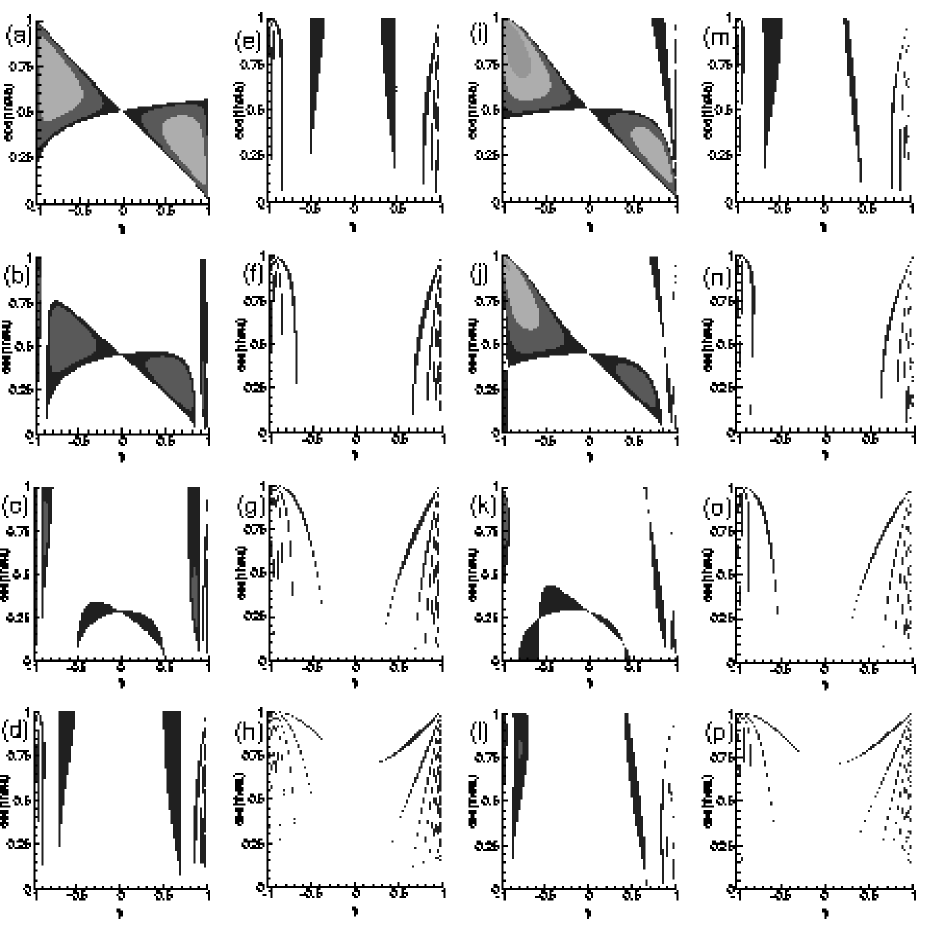
Figure 3: Instability domain of $\mathbf{a}(t)$ in the classical EB equations (Figs.(a)-(h) with $\Upsilon_{0}=1$) and the LAEB$-\alpha$ model (Figs. (i)-(p) with $\Upsilon_{0}=5/4$) for rotation parameter $\zeta=2$ (no rotation) and various values of buoyancy parameter $\chi$: (a),(i) 0; (b),(j) 1/4; (c),(k) 3/4; (d),(l) 2; (e),(m) 3; (f),(n) 5; (g),(o) 8; and (h),(p) 14. Regions in white represent parameter values for which the amplitude $\mathbf{a}$ is bounded in time. For all other regions, the amplitude grows exponentially in time. The contour lines are level lines of the Lyapunov-like growth rate with the same coloring in each figure. The fact that some of the fingers appear to be disjoint regions is merely an artifact of numerical simulation and data visualization. See the text for a description of the behavior of each individual subfigure. The values of $N^{2}$ and $\Omega$ in (a)-(h) differ from those in (i)-(p) due to the fact that $\chi$ and $\zeta$ are similarity variables (see (23)).

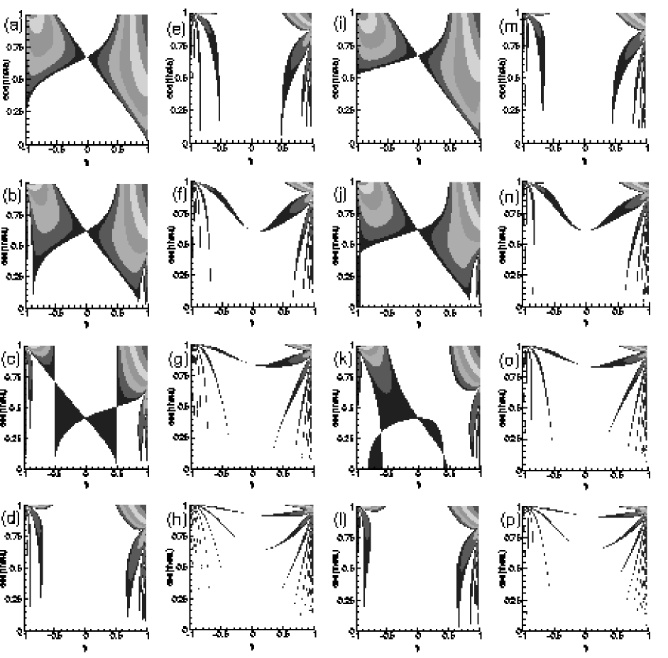
Figure 4: The instability domains of $\mathbf{a}(t)$ in the classical EB equations (Figs.(a)-(h) with $\Upsilon_{0}=1$) and the LAEB$-\alpha$ model (Figs.(i)-(p) with $\Upsilon_{0}=5/4$) for rotation parameter $\zeta=3/2$ and the same values of buoyancy parameter $\chi$ as in Fig. 3: (a),(i) 0; (b),(j) 1/4; (c),(k) 3/4; (d),(l) 2; (e),(m) 3; (f),(n) 5; (g),(o) 8; and (h),(p) 14. Note the presence of a stable band in (d)-(e) and (l)-(m), corresponding to $1<\sqrt{\chi}<2$ (see (29)).

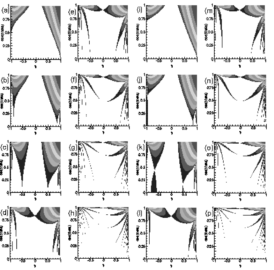
Figure 5: The instability domains of $\mathbf{a}(t)$ in the classical EB equations (Figs.(a)-(h) with $\Upsilon_{0}=1$) and the LAEB$-\alpha$ model (Figs.(i)-(p) with $\Upsilon_{0}=5/4$) for rotation parameter $\zeta=3/4$ and the same values of buoyancy parameter $\chi$ as in Fig. 3: (a),(i) 0; (b),(j) 1/4; (c),(k) 3/4; (d),(l) 2; (e),(m) 3; (f),(n) 5; (g),(o) 8; and (h),(p) 14. Note that since $\zeta<1$, we have a stable band of flows in (a)-(c) and (i)-(k), where $\chi<1$ (see (30)).

The first conclusion is that stratification and rotation increases the angle of critical stability (decreases $\cos\theta$). The different values of $n$ indicate the primary, secondary, tertiary, etc., instability domains. These different instability domains, or fingers, have been extensively studiedmiya:fuku:92 ; miya:93 ; fab:holm:04a . The principal finger, $n=1$, is the main instability domain for elliptic instability, and it is call the ‘subharmonic frequency.’ The secondary finger, $n=2$, corresponds to a resonance phenomenon with internal gravity waves, and thus is called the ‘fundemental frequency.’ The remaining fingers, $n=3,4,\ldots$, naturally are referred to as ‘superharmonic frequencies.’ In the absence of statification, only the subharmonic frequency ($n=1$) is physically interesting from the viewpoint of elliptic instability, although rotation increases the width of the other frequencies. (These fingers are displayed in Figs. 3-5 below.) Since the expression for $\cos\theta$ is independent of $\Upsilon_{0}$ explicitly, the second conclusion we draw is that the LAEB$-\alpha$ model has no effect on the circular case, provided that the values of $N^{2}$ and $\Omega$ change as $\alpha$ changes so that $\chi$ and $\zeta$ remain fixed.

IV.2 Slightly elliptic streamlines–perturbation analyses

The parameter values which yield critical stability for the circular case will produce instability in the elliptic case for small eccentricities. We derive an analytical expression for the leading order growth rate of this instability to $O(\gamma^{2})$, defined for the LAEB$-\alpha$ model as

$$\sigma\equiv\frac{1}{2(\Upsilon_{0}|\mathbf{a}|^{2}+N^{2}\hat{b}^{2})}\frac{d}{dt}\Big{(}\Upsilon_{0}|\mathbf{a}|^{2}+N^{2}\hat{b}^{2}\Big{)}.$$ (27)

This is a natural extension of the definition given by Kerswellkers:02 for $\Upsilon_{0}=1$, and differs slightly from that in previous work on the LANS$-\alpha$ modelfab:holm:03 ; fab:holm:04a . By taking the dot product of (18) with $\mathbf{a}$, multiplying (19) by $N^{2}\hat{b}$, and adding, we find that the following expression for $\sigma$:

$$\sigma=\frac{-\mathbf{a}^{T}\cdot\mathcal{S}^{T}\cdot(\Upsilon_{0}\mathbf{a})}{2\Upsilon_{0}}=-\gamma a_{1}a_{2}$$

valid for all $\gamma$, where $a_{1,2}$ are the first and second components of $\mathbf{a}$, respectively. We insert the circular solutions (that is, for $\gamma=0$) into the above equation, say $\mathbf{a}_{1}$ and $\hat{b}_{1}$, and average over a period of the solutions. Typicallywal:90 , the average will vanish except when $\omega\pm 1=0$, a condition which again yields (26). A maximum is attained when $\phi=\pm\pi/4$, yielding

$$\sigma_{\text{max}}=\Big{(}\frac{9}{16}\times\frac{4(n^{2}-\chi)(\zeta+n)}{9\Upsilon_{0}n^{2}(\zeta^{2}-\chi)}\Big{)}\gamma+O(\gamma^{2}).$$ (28)

We see that for base flows with small deviations from circular, that is, for flows with $|\gamma|\ll 1$, the growth rates are linear in the eccentricity. Of particular interest is the fact that $\sigma_{\text{max}}$ is a function of all three parameter $\chi$, $\zeta$, and $\Upsilon_{0}$, rather than just the first two. We conclude that although properly adjusting the Brunt-Väisälä frequency and Rossby number preserves the effects the model has on circular flows, the growth rate in the LAEB$-\alpha$ model is a decreasing function of the model parameter $\Upsilon_{0}$. Numerical simulations below will show that for moderate and large eccentricities, the effect is more dramatic. In particular, the subharmonic finger ($n=1$) has a maximum growth rate of $\sigma_{\text{max}}=\gamma/(2\Upsilon_{0})$, which occurs at $\zeta=1$ ($\Omega=-1/2$). For this parameter value, the critical angle is $\cos\theta=1$, that is, when the wave vector is parallel to the ellipse’s axis of rotation. This is referred as the zero tilting vorticitycambon:94 ; leb:03 . We will expand on this case in a separate section.

The expression for the critical angle (26) separates the parameter space into four distinct regions. We describe each region by its characteristic behavior. We preserve the $\zeta$ and $\chi$ notation since the behavior will remain unchanged under the redefinition of these two variables for the LAEB$-\alpha$ model in the next section.

1. Both the numerator and denominator of the radicand have the same sign and the ratio is less than unity. For parameter values in this region, we have $\cos\theta<1$. Thus, slight perturbations in the columnar vortex’s eccentricity from circular will yield exponentially growing amplitudes. This is due to the fact that the fingers touch the line $\gamma=0$ at a point (a consequence of parametric resonance and the fact that $\gamma=0$ is stable). For a given finger with index $n$, we have that either $\cos\theta\to 0^{+}$ as $\chi\to(n^{2})^{-}$ and it vanishes for larger values of $\chi$ or $\cos\theta\to 1^{-}$ as $\chi\to\infty$, in which case it never vanishes.

2. Both the numerator and denominator of the radicand are positive and the ratio is greater than unity. Parameter values in this region correspond to $\cos\theta>1$ and experience a window of nonzero eccentricities for which the Kelvin waves are bounded (i.e. stability). If we could extend the parameter plane to include values of $\cos\theta$ larger than unity, then the fingers which fall into region (II) would also experience instability. The unique property here is that $\cos\theta\to+\infty$ as $\chi\to(\zeta^{2})^{-}$.

3. Both the numerator and denominator of the radicand are negative and the ratio is greater than unity. For these parameter values, the fingers whose index corresponds to $n<\zeta$ have vanished and will not reappear. They enter this region at $\chi=(\zeta^{2})^{+}$ with $\cos\theta=+\infty$ and has the feature that $\cos\theta\to 1^{+}$ as $\chi\to\infty$.

4. The numerator and denominator have different signs. Parameter values which fall into this region are particularly interesting. For these values, the instability domains align themselves vertically in the $(\gamma,\cos\theta)-$plane rather than horizontally or diagonally towards $\cos\theta=1$, $\gamma=0$.

Figures 1 and 2 shows the four regions in the $(\chi,n)$ and $(\chi,\zeta)$ parameter planes, respectively, and Figs. 3-5 show numerical simulations which exhibit the described behavior of the fingers. These figures show domains of stable and unstable behavior as a function of buoyancy $\chi$ and rotation $\zeta$ parameters for elliptic instabilities of various orders; subharmonic ($n=1$), fundamental ($n=2$), and superharmonic ($n=3,4,\ldots$). In particular, subfigures (a)-(h) show the results for the EB equations ($\Upsilon_{0}=1$) and subfigures (i)-(p) show the effects of the LAEB$-\alpha$ model for the same values of the similarity variables $\zeta$ and $\chi$.

Figure 1 shows the different regions for a fixed representative value of $\zeta$. The horizontal and vertical lines which separate the different regions intersect on the parabola at the point $(\zeta^{2},\zeta)$. As $\zeta$ decreases, the intersection point slides down the parabola towards the origin and the unstable fingers in region (I) stabilize and enter region (II). The figure, as drawn, indicates that the fingers corresponding to the subharmonic ($n=1$) and fundamental ($n=2$) frequencies live in region (I) for $n<\sqrt{\chi}$, in region (IV) for $\sqrt{\chi}<n<\zeta^{2}$, and in region (III) for $n>\zeta^{2}$. These fingers will be unstable in (I) and vanish in (IV) and (III). In contrast, the fingers for the superharmonic frequencies $n\geq 3$ live in region (II) for $n<\zeta^{2}$, region (IV) for $\zeta^{2}<n<\sqrt{\chi}$, and finally region (I) for $n>\sqrt{\chi}$. These fingers are aligned diagonally in the $(\gamma,\cos\theta)$-plane for region (II) and vertically for region (IV), and then meet at the line $\gamma=0$ as parameter values enter region (I).

We deduce two stability criteria from Figs. 1-2 and (26). First, for parameter values satisfying $\lfloor\zeta\rfloor<\sqrt{\chi}<\lceil\zeta\rceil$, or in original variables,

$$\Big{\lfloor}\frac{2|\Omega+1|}{\Upsilon_{0}}\Big{\rfloor}<\sqrt{\frac{N^{2}}{\Upsilon_{0}}}<\Big{\lceil}\frac{2|\Omega+1|}{\Upsilon_{0}}\Big{\rceil},$$ (29)

where $\lfloor x\rfloor$ and $\lceil x\rceil$ the floor and ceiling of $x$, respectively, the flow is always stable. Here, floor and ceiling refer to rounding the the nearest integer less than and greater than the current value, respectively. Essentially, (29) follows from the fact that none of the fingers live in region (I) for these parameter values. This criterion is analogous to the nonresonance stability criterion $1/2\leq N/(2\Omega)\leq 2$ for forced turbulence in three-dimensional rotating, stably stratified flow in the Boussinesq approximationsmith:wal:02 . (Note that their equation for the buoyancy differs from ours.) For $\zeta=\sqrt{5}$ in Fig. 1, this corresponds to $2<\sqrt{\chi}<3$. The second stability criterion is that all of the fingers will live in region (II) when

$$-\frac{\Upsilon_{0}}{2}<\Omega+1<\frac{\Upsilon_{0}}{2}\,\,\text{for}\,\,N^{2}<\Upsilon_{0},$$ (30)

Within this window, the flow is stable for slight perturbations in $\gamma$. This means counter rotation stabilizes the flow, when the Brunt-Väisälä frequency is sufficiently low. Contrast this with Leblanc’sleb:03 stability criterion for the EB equations ($\Upsilon_{0}=1$), which says that for $\Omega=-1$, the flow is stable for parameter values satisfying $N^{2}\leq 1-\gamma^{2}$. (In (30), $\gamma=0$.)

IV.3 Two-dimensional perturbations

IV.3.1 $\cos\theta=1$

The case $\cos\theta=1$, that is when the wave vector of the Kelvin wave is parallel to the axis of rotation, also can be analyzed analytically. As mentioned before, this is referred to as the zero tilting vorticity because the vorticity of the ellipse-wave system is merely stretched rather than tilted. This follows from the fact that $\mathbf{k}=[0,0,1]^{T}$, which, because of transversality (12), forces $\mathbf{a}=[a_{1},a_{2},0]$. The resulting equations yield $\hat{b}(t)=\text{const.}$, and

$$\dot{a}_{1}+(1-\zeta+\gamma)a_{2} =0,$$

$$\dot{a}_{2}-(1-\zeta-\gamma)a_{1} =0.$$ (31)

It follows that no exponential growth of the solution of (20) will occur for parameter values satisfying

$$(1-\zeta)^{2}-\gamma^{2}\geq 0.$$ (32)

IV.3.2 $\cos\theta=0$

We perform a separate investigation for the case $\cos\theta=0$, that is, when the wave vector lies in the plane of the flow. As was the case for $\cos\theta=1$, the equations decouple such that the equations for $a_{1,2}$ are independent of $a_{3}$ and $\hat{b}$, and vice-versa. The equations for $a_{1,2}$ are exactly those for the LANS$-\alpha$ model, and the equations for $a_{3}$ and $\hat{b}$ can be rewritten as a single Schrödinger equation:

$$\ddot{v}+\frac{N^{2}}{\Upsilon}v=0,$$ (33)

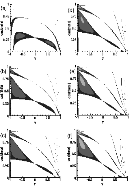
Figure 6: Instability domain of $\mathbf{a}(t)$ for rotation parameter $\zeta=3$, buoyancy parameter $\chi=1/4$, and various model parameter $\Upsilon_{0}$: (a) 1 (the EB equations), (b) 3/2, (c) 2, (d) 11/4, (e) 4, and (f) 6. The behavior of the instability regions is essentially the same in all figures for $|\gamma|\ll 1$.

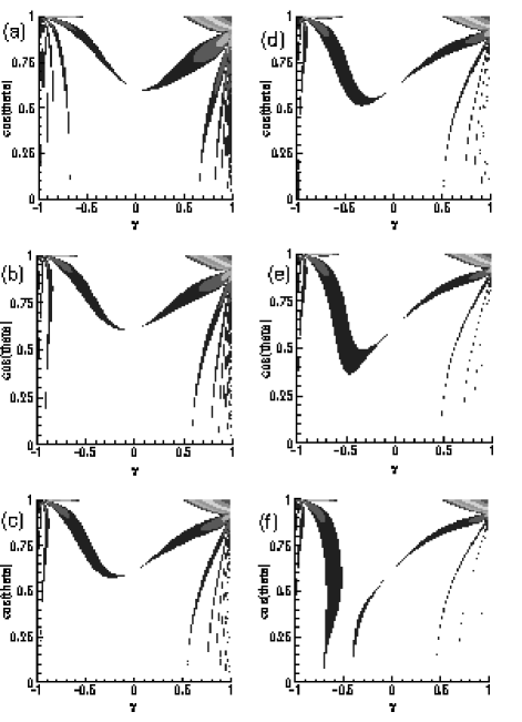
Figure 7: Instability domain of $\mathbf{a}(t)$ for rotation parameter $\zeta=3/2$, buoyancy parameter $\chi=5$, and various model parameter $\Upsilon_{0}$: (a) 1 (the EB equations), (b) 3/2, (c) 2, (d) 11/4, (e) 4, and (f) 6. Again, the behavior of the instability regions is essentially the same in all figures for $|\gamma|\ll 1$.

where $v=\Upsilon a_{3}$ and overhead dot denotes a time derivative. For the EB case, $\Upsilon(t)=1$, and the solutions are purely periodic and bounded, i.e., stable. In fact, this case is critically stable in the sense that any slight perturbation of the wave vector in the third dimension ($\cos\theta>0$) could result in Kelvin waves with exponentially growing amplitudes miya:fuku:92 ; miya:93 . This corresponds to the fingers touching the $\gamma-$axis in the shape of a cusp, seen in subfigures (a)-(h) in Figs. 3-5, Fig. 6a, and Fig. 7a, as predicted by Floquet theory. For the LAEB$-\alpha$ model, (33) is once again a Floquet problem. Comparison of numerical simulations of the full $4\times 4$ system in (20) and that in (33) yield exactly the same growth rates over the same parameter ranges. We conclude, then, that buoyancy coupled with the model parameter $\Upsilon_{0}$ is the cause of this instability. This is illustrated in subfigures (i)-(p) of Figs. 3-5, and in Fig. 8. Numerical simulations suggest that these two-dimensional instabilities exist only for $\chi<2$, even for extra-ordinarily large values of $\Upsilon_{0}$.

IV.4 Elliptic streamlines–numerical simulations

Figures 3-5 display the instability domains for a representative set of $\zeta$ and $\chi$. We reiterate that subfigures (a)-(h) correspond to the classic EB equations ($\Upsilon_{0}=1$), and subfigures (i)-(p) correspond to the LAEB$-\alpha$ model for parameter value $\Upsilon_{0}=5/4$. The figures are set side-by-side so that the reader can easily see the effects the model has on the classical solutions. We see the large number of instability fingers, or Arnold tongues, corresponding to various values of $n$ in (26). The previously described shift of fingers into and out of regions (I)-(IV) is also clearly seen.

We describe the behavior of the fingers in Fig. 3, the case $\zeta=2$ ($\Omega=0$), in detail. For $\chi=0$ (Fig. 3a,i), the critical angles are $\cos\theta=1/2$ (subharmonic) and $\cos\theta=1$ (fundamental), the latter being true for all $\chi$. The subharmonic finger lives in region (I), and the fundamental finger lives on the boundary between regions (I) and (II). As $\chi$ increases towards unity (Figs. 3b,c,j,k), the subharmonic finger shifts in the parameter plane towards $\cos\theta=0$. In the range $1<\chi<4$ (Figs. 3d,e,l,m), the finger corresponding to the subharmonic frequency has vanished, that is, it has entered region (IV). We conjecture that the vertically aligned finger in these pictures, which collapses on the line $\gamma=0$ at $\chi=4$, corresponds to the fundamental frequency ($n=2$). In the range $4<\chi<9$ (Figs. 3f,g,n,o), the fingers corresponding to the superharmonic frequencies ($n\geq 3$) have shifted from region (II) to region (IV) and appear to be vertical. For $\chi>9$ (Figs. 3h,p), the fingers corresponding to the first superharmonic frequency ($n=3$) have shifted from region (IV) to region (I) and meet at the prescribed critical angle (26) along $\gamma=0$. Once again, the flow is unstable for infinitesimally small, non-zero eccentricities. Seen is the second superharmonic ($n=4$) shifting in the plane. What cannot be seen is the fact that the finger for the subharmonic frequency ($n=1$) has disappeared into region (III), never to return. Not shown is the fact that the second superharmonic frequency’s fingers ($n=4$) will touch on $\gamma=0$ at $\chi=16$. Similarly for the third superharmonic at $\chi=25$, and so on. The fixed value of $\zeta=2$ satisfies (32) for all $\gamma$, and thus the flow is always stable on the line $\cos\theta=1$. The vertical lines in Fig. 3b-e,i-m, corresponding to the second finger, do not touch the line $\cos\theta=1$. Rather, they curve sharply near that line, meeting it only at $\gamma=1$. This behavior is difficult to resolve numerically. However, we verify that this case is stable on the line $\cos\theta=1$ itself. The behavior of the fingers is similar in the presence of rotation (Figs. 4 and 5).

Figure 4 shows corresponding contour plots for the parameter value $\zeta=3/2$. We see that the primary finger (subharmonic frequency) touches the $\gamma=0$ line at $\cos\theta=2/3$ (Figs. 4a,i). Note that for $1<\chi<4$ (Figs. 4d,e,l,m), there are eccentric flows for which the Kelvin waves are stable. This is because (29) is satisfied for these parameter values. The value of $\zeta$ here satisfies (32) only for $-1/2<\gamma<1/2$. Outside of this region, the flow is unstable on the line $\cos\theta=1$. We see that in all images, this fact holds true. Any visual deviation from this stability band is a consequence of the plotting program. We verify numerically that the band does not change width as a function of $\Upsilon_{0}$ or $\chi$.

The behavior for $\zeta=3/4$, shown in Fig. 5, is similar to the previous cases. Note that the main difference here is the stable band of eccentric flows for $\chi<1$ (Figs. 5a-c,i-k), where (30) is satisfied. Furthermore, we see pairs of fingers enter region (I) as predicted–the primary (subharmonic) for $\chi>1$, the secondary (fundamental) for $\chi>4$, and the tertiary (first superharmonic) for $\chi>9$ (Figs. 3d-h,l-p).

Remark. Previous workfab:holm:04a commented on the fact that there is a remarkable similarity between the effects of counter-rotation, i.e. decreasing $|\Omega+1|$, and increasing the parameter $\alpha$ on elliptic instability. This similarity is better understood by choosing $\zeta=2|\Omega+1|/(1+\alpha^{2}\beta^{2})$ as a similarity variable. Numerical simulations show that the growth rates obtained by maximizing over the $(\gamma,\cos\theta)$-plane are roughly constant functions of $\Upsilon_{0}$ for randomly chosen fixed values of $\chi$ and $\zeta$ satisfying $\zeta<1$. This is because the maximum typically occurs on the finger associated with the subharmonic frequency ($n=1$). Again, this indicates that the LAEB$-\alpha$ model will preserve the basic characteristics of elliptic instability by properly adjusting the Rossby number and the Brunt-Väisälä frequency. When $\zeta>1$, however, the finger associated with the subharmonic frequency has vanished, and the maximum growth rates vary due to the presence of other frequencies. Since the model alters the shape of the fingers associated with these frequencies as well as the associated Lyapunov exponents for moderate and large eccentricities, there is no reason to expect that the growth rate remain constant.

V Anisotropic LAEB$-\alpha$ model

We now examine the effects of anisotropy in the third component of the velocity field $\mathbf{v}$. We do this by altering the definition of the transported velocity $\mathbf{v}$ from $\mathbf{v}=(1-\alpha^{2}\Delta)\mathbf{u}$ to

$$\mathbf{v}=(1-\alpha^{2}(\partial^{2}_{xx}+\partial^{2}_{yy}+\epsilon^{2}\partial^{2}_{zz}))\mathbf{u}.$$ (34)

Here, $\epsilon$ measures the anisotropy of the transported velocity field $0\leq\epsilon\leq 1$. For $\epsilon=1$, we regain the results of the previous section. From the view of elliptic instability, the main difference is the change in the definition of $\Upsilon(t)$ from (11) to

$$\Upsilon(t)=1+\alpha^{2}\beta^{2}(k_{1}^{2}(t)+k_{2}^{2}(t)+\epsilon^{2}k_{3}^{2}(t)).$$ (35)

The theory for the isotropic LAEB$-\alpha$ model in the parameter regime $|\gamma|\ll 1$ remains intact using the similarity variables given in (23) with

$$\Upsilon_{0}=1+\alpha^{2}\beta^{2}(1-(1-\epsilon^{2})\cos^{2}\theta).$$ (36)

Effectively, anisotropy in the third component will reduce the value of $\Upsilon_{0}$ (since $1-(1-\epsilon^{2})\cos^{2}\theta\leq 1$). Numerical simulations verify that there are no changes along the line $\gamma=0$, trival differences in the region $|\gamma|\ll 1$, and possibly noticable differences for $\gamma\approx 1$, the last of which occur only for values $\alpha^{2}\beta^{2}>1$. The main distinction lies in the fact that each subfigure of Figs. 3-5 corresponds to fixed values of $\Omega$ and $N^{2}$, whereas similar figures using (23) with (36) would result in different horizontal lines, that is, each value of $\cos\theta$, corresponding to different $\Omega$ and $N^{2}$ values within a subfigure.

VI Conclusions

We have studied the effects of a turbulence closure model for the Euler-Boussinesq equations on elliptic instability. We found a trade-off in the effects of turbulence, in that the model can increase the width of one stability band (see (29)) while simultaneously decreasing the width of another (see (30)). This occurs because of wave number dependence is introduced when the smoothing operation (with lengthscale $\alpha$) is applied in developing a mean model of turbulence. We expect that other turbulence models will show similar tendencies, although our earlier work fab:holm:04a shows that the magnitudes and functional forms of these tendencies may vary from one turbulence model to another.

The LAEB$-\alpha$ model considered here has the advantage of preserving the main features of classic elliptic instability analysis for circular flows, up to rescaling the stability conditions in terms of rotation and buoyancy frequencies by certain factors involving the nondimensional wavenumber parameter $\Upsilon_{0}$, which may also contain anisotropic information as well. This wavenumber parameter is made nondimensional by using the lengthscale (turbulence correlation width) in the LAEB$-\alpha$ model. The similarity property and the preservation of structure under appropriate rescaling the frequencies by $\Upsilon_{0}$ has allowed a complete analysis of the mean effects of turbulence on the elliptic instability, when viewed as an exact nonlinear CC solution of the LAEB$-\alpha$ model. This similarity property also reveals how the smoothing introduced in developing the turbulence model interacts with the physical effects of rotation and buoyancy, which are vital for understanding turbulence in geophysical flows. One outstanding question remains, which is something of a technical detail. Namely, we would still like to know the mechanism by which the turbulence model affects the resonance regions seen in Figs. 6-7 for elliptical flows of high eccenticity. These are similarity breaking effects of the LAEB$-\alpha$ turbulence model. They arise because of the introduction of the length scale $\alpha$ and cannot be removed by rescaling the other parameters in the problem. Anisotropy in the $z-$component of the velocity field amplifies these effects. These effects tend to occur as the shear in the flow (represented by $\gamma$) becomes more pronounced. In flows of such high eccenticity, coursening at the correlation length $\alpha$ in the turbulence model may be exhibiting different effects than for small eccentricity, because of the higher anisotropy of these flows in the plane of the strain flow. The derivation of the LAEB$-\alpha$ model assumes isotropy of the fluctuations in all coordinates, which does not hold in the case of flows with high eccentricity. Perhaps another version of the model–one which would allow for strong planar anisotropy in the statistical correlations of turbulent Lagrangian fluctuations with their mean trajectories–would not show such pronounced effects at high eccentricity.

Additionally, the LAEB$-\alpha$ model introduces a band of unstable flows in the parameter regime $\cos\theta=0$, where the wave vector lies in the plane of the flow. This is a direct consequence of the presence of buoyancy. Classically, this parameter regime is critically stable.

Finally, we note that Miyazaki and Adachimiya:ada:98 were able to extend the result of Lifschitz and Fabijonaslif:fab:96 to stratified circular flows. Namely, the stable parameter values for the Kelvin wave in the circular case ($\gamma=0$) are unstable with respect to high-frequency perturbations. We conjecture that the same holds true for the LAEB$-\alpha$ model.

Appendix A Recasting Eq. (20) as a pair of Schödinger equations

We recast (20) as a coupled pair of Schödinger equations in the spirit of Ref. bay:holm:lif:96, for all base flows for which the matrix $\mathcal{S}$ has the form

$$\mathcal{S}=\begin{pmatrix}\mathcal{S}_{\perp}&\mathbf{0}_{2}\\ \mathbf{0}_{2}^{T}&0\end{pmatrix}.$$

Here $\mathbf{0}_{2}$ is the zero vector in $\mathbb{R}^{2}$ and $\mathcal{S}_{\perp}$ is a $2\times 2$ matrix. Incompressibility demands that $\operatorname{tr}(\mathcal{S}_{\perp})=0$.

We decompose the amplitude vector $\mathbf{a}$ and the wave vector $\mathbf{k}$ into components which are perpendicular and parallel to the axis of rotation:

$$\mathbf{k}=\begin{pmatrix}\mathbf{k}_{\perp}\\ k_{\parallel}\end{pmatrix},\qquad\mathbf{a}=\begin{pmatrix}\mathbf{a}_{\perp}\\ a_{\parallel}\end{pmatrix},\qquad\mathbf{\Omega}=\begin{pmatrix}\mathbf{0}_{2}\\ \Omega\end{pmatrix},$$

where $\mathbf{0}_{2}$, $\mathbf{k}_{\perp}$ and $\mathbf{a}_{\perp}$ are vectors in $\mathbb{R}^{2}$. Equations (12) and (17)-(19) take the form

$$\mathbf{k}_{\perp}^{T}\cdot\mathbf{a}_{\perp}+k_{\parallel}a_{\parallel}=0,$$

$$d_{t}\mathbf{k}_{\perp}=-\mathcal{S}_{\perp}^{T}\cdot\mathbf{k}_{\perp},\qquad d_{t}k_{\parallel}=0,$$

$$d_{t}(\Upsilon\mathbf{a}_{\perp})=\frac{N^{2}k_{\parallel}\mathbf{k}_{\perp}}{|\mathbf{k}|^{2}}\,\hat{b}$$

$$\phantom{X}-\Big{(}(\Upsilon-1)\mathcal{S}_{\perp}^{T}+\mathcal{S}_{\perp}+2\Omega\mathcal{R}-\frac{\mathbf{k}_{\perp}\mathbf{k}_{\perp}^{T}\cdot\mathcal{M}}{|\mathbf{k}|^{2}}\Big{)}\cdot\mathbf{a}_{\perp},$$

$$d_{t}(\Upsilon a_{\parallel})=\frac{k_{\parallel}\mathbf{k}_{\perp}^{T}\cdot\mathcal{M}}{|\mathbf{k}|^{2}}\cdot\mathbf{a}_{\perp}+\Big{(}-N^{2}+\frac{N^{2}k_{\parallel}^{2}}{|\mathbf{k}|^{2}}\Big{)}\,\hat{b},$$

$$d_{t}\hat{b}=a_{\parallel}.$$

Here,

$$\mathcal{M}=(\Upsilon+1)\mathcal{S}_{\perp}+(\Upsilon-1)\mathcal{S}_{\perp}^{T}+2\Omega\mathcal{R},$$

$$\mathcal{R}=\begin{pmatrix}0&-1\\ 1&0\end{pmatrix}.$$

Consider the transformations

$$p=\frac{|\mathbf{k}|}{|\mathbf{k}_{\perp}|}\mathbf{k}_{\perp}^{T}\cdot(\Upsilon\mathbf{a}_{\perp})=-\frac{|\mathbf{k}|}{|\mathbf{k}_{\perp}|}k_{\parallel}(\Upsilon a_{\parallel}),$$

$$q=\frac{|\mathbf{k}|}{|\mathbf{k}_{\perp}|}\left(\mathbf{k}\times(\Upsilon\mathbf{a})\right)_{\parallel},\qquad r=\frac{|\mathbf{k}|}{|\mathbf{k}_{\perp}|}\,\hat{b}.$$

Here, $(\mathbf{u})_{\parallel}$ represents the third component of a vector $\mathbf{u}$. The system of equations satisfied by these variables is

$$\frac{d}{dt}\begin{pmatrix}p\\ q\\ r\end{pmatrix}=\begin{pmatrix}K&H&M_{1}\\ -Q&-K&0\\ -M_{2}&0&-K\end{pmatrix}\begin{pmatrix}p\\ q\\ r\end{pmatrix}.$$ (37)

where

$$K =\frac{d}{dt}\left(\ln\Big{(}\frac{|\mathbf{k}_{\perp}|}{|\mathbf{k}|}\Big{)}\right),\quad H=\frac{k_{\parallel}^{2}\mathbf{k}_{\perp}^{T}\cdot\mathcal{M}\cdot\mathcal{R}^{T}\cdot\mathbf{k}_{\perp}}{\Upsilon|\mathbf{k}|^{2}|\mathbf{k}_{\perp}|^{2}},$$

$$Q =\frac{1}{\Upsilon}(W+2\Omega),\quad W=(\operatorname{curl}\,(\mathcal{L}\cdot\mathbf{x}))_{\parallel}=(L_{21}-L_{12})$$

$$M_{1} =\frac{k_{\parallel}N^{2}|\mathbf{k}_{\perp}|^{2}}{|\mathbf{k}|^{2}},\quad M_{2}=\frac{1}{k_{\parallel}\Upsilon}.$$

We eliminate the variable $p$ from the problem, recasting the above system as a pair of second order Schrödinger equations for $q$ and $r$ (overhead dot denotes differentiation with respect to time):

$$\ddot{q}-\frac{\dot{Q}}{Q}\dot{q}+\Big{[}QH+\dot{K}-K^{2}-\frac{\dot{Q}}{Q}K\Big{]}\,q+QM_{1}\,r=0$$

$$\begin{split}\ddot{r}+K\dot{r}+[\dot{K}+M_{1}M_{2}]\,r-\frac{\dot{M}_{2}+M_{2}K}{Q}\,\dot{q}\phantom{+XXX}\\ -\Big{[}\frac{\dot{M}_{2}K+M_{2}K^{2}}{Q}+M_{2}H\Big{]}\,q=0\end{split}$$

The results for the LANS$-\alpha$ model are obtained by setting $N^{2}=0$ (corresponding to $M_{1}=0$) and ignoring the equation for $r$. The results for the Navier-Stokes equationsbay:holm:lif:96 are regained by setting $\Upsilon=1$.

Figure 1: The $(\chi,n)$ parameter plane for the representative fixed value $\zeta=\sqrt{5}$. The roman numerals indicate different regions described in the text. Region (I) corresponds to real values of $\cos\theta$ which are less than unity. Parameter values in this region will yield exponential growth of $\mathbf{a}(t)$ for small values of eccentricity $\gamma$. Regions (II) and (III) correpsond to real values of $\cos\theta$ greater than unity, and region (IV) correpsonds to imaginary values of $\cos\theta$. Parameter values which fall into these regions yield windows of eccentricity values for which the disturbance is always stable. The curves separating different regions are the dashed curves given by the equations $n=\sqrt{\chi}$ (the parabola), $\chi=\zeta^{2}$ (the vertical line), and $n=\zeta$ (the horizontal line). These curves separate the various types of elliptic instability behavior in the $(\chi,n)$ parameter plane into four regions, according to Eq. (26) for the critical angle.

Figure 2: The $(\chi,\zeta)$ parameter plane for the representative fixed value $n=3$, with the different regions described in the text. This figure describes the behavior of the tertiary finger for different values of $\zeta$ and $\chi$. The regions are separated by the dashed curves given by the parabola $\chi=\zeta^{2}$, the vertical line $\chi=n^{2}$, and the horizontal line $\zeta=n$.

Figure 8: The growth rate for the case $\cos\theta=0$ for $\chi=3/4$ and $\zeta=3$, and for values of $\Upsilon_{0}$ in the range $1\leq\Upsilon_{0}\leq 4$. For $\Upsilon_{0}=1$, the Lyapunov exponent is identically zero. The exponent is immediately non-zero for $\Upsilon_{0}>1$, and shifts to the left as the parameter increases. For larger values of $\Upsilon_{0}$, the growth rates approach an asymptotic limit, which is slightly to the left of the curve corresponding to $\Upsilon_{0}=4$ shown in the figure.

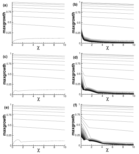
Figure 9: The growth rate maximzed over the $(\cos\theta,\gamma)$ plane as a function of $\chi$ for various $\zeta$ and $\Upsilon_{0}$: (a-b) $\Upsilon_{0}=1$, (c-d) $\Upsilon_{0}=3/2$, (e-f) $\Upsilon_{0}=4$. The figures in the left column correspond to $\zeta$ values satisfying $0\leq\zeta\leq 1$, increasing from bottom to top. Similarly, the figures in the right column correspond to $\zeta$ values satisfying $\zeta>1$, increasing from top to bottom. Notice that as $\zeta\to\infty$, the growth rates approach an asymptotic limit for all $\Upsilon_{0}$. This is in accordance with the Taylor-Proudman theorem. Notice further the development of a “bump” for $\Upsilon_{0}>1$, when $\zeta=0$ (the bottom-most curve in the figures in the left column) and as $\zeta\to\infty$ (the bottom-most curves in the figures in the right column).

References

- (1) B. R. Fabijonas and D. D. Holm, “Mean effects of turbulence on elliptic instability,” Phys. Rev. Lett. 90, 124501 (2003).
- (2) B. R. Fabijonas and D. D. Holm, “Craik-Criminale solutions and elliptic instability in nonlinear-reactive closure models for turbulence,” Phys. Fluids 16, 853 (2004).
- (3) D. D. Holm, J. E. Marsden, and T. S. Ratiu, “Euler-Poincaré models of ideal fluids with nonlinear dispersion,” Phys. Rev. Lett. 80, 4173 (1998).
- (4) D. D. Holm, “Fluctuation effects on 3d lagrangian mean and eulerian mean fluid motion,” Physica 133D, 215 (1999).
- (5) D. D. Holm, J. E. Marsden, and T. S. Ratiu, “The Euler-Poincaré equations in geophysical fluid dynamics,” in Large-Scale Atmosphere-Ocean Dynamics 2: Geometric Methods and Models, edited by J. Norbury and I. Roulstone, pages 251–299, Cambridge University Press, 2002.
- (6) J. Leray, “Sur le mouvement d’un liquide visqueux emplissant l’espace,” Acta Math. 63, 193 (1934).
- (7) Lord Kelvin, “Stability of fluid motion: rectilinear motion of viscous fluid between two parallel plates,” Phil. Mag. 24, 188 (1887).
- (8) B. J. Bayly, “Three-dimensional instability of elliptical flow,” Phys. Rev. Lett. 57, 2160 (1986).
- (9) A. D. D. Craik and W. O. Criminale, “Evolution of wavelike disturbances in shear flows: a class of exact solutions of the Navier-Stokes equations,” Proc. R. Soc. London A 406, 13 (1986).
- (10) A. D. D. Craik, “A class of exact solutions in viscous incompressible magnetohydrodynamics,” Proc. R. Soc. London A 417, 235 (1988).
- (11) A. D. D. Craik, “The stability of unbounded two- and three-dimensional flows subject to body forces: some exact solutions,” J. Fluid Mech. 198, 275 (1989).
- (12) F. Waleffe, “On the three-dimensional instability of strained vortices,” Phys. Fluids A 2, 76 (1990).
- (13) T. Miyazaki and Y. Fukumoto, “Three-dimensional instability of strained vortices in a stably stratified fluid,” Phys. Fluids 4, 2515 (1992).
- (14) R. R. Kerswell, “Elliptical instabilities of stratified, hydromagnetic waves,” Geophys. Astrophys. Fluid Dynam. 71, 105 (1993).
- (15) T. Miyazaki, “Elliptical instability in a stably stratified rotating fluid,” Phys. Fluids 5, 2702 (1993).
- (16) S. Leblanc, “Internal wave resonances in strain flows,” J. Fluid Mech. 477, 259 (2003).
- (17) R. R. Kerswell, “Elliptical instability,” Annu. Rev. Fluid Mech. 34, 83 (2002).
- (18) V. A. Yakubovich and V. M. Starzhinskii, Linear Differential Equations with Periodic Coefficients, Wiley, 1967.
- (19) C. Cambon, J. .P Benoît, L. Shao, and L. Jacquin, “Stability analysis and large eddy simulation of rotating turbulence with organized eddies,” J. Fluid Mech. 278, 175 (1994).
- (20) L. M. Smith and F. Waleffe, “Generation of flow large scales in forced rotating stratified turbulence,” J. Fluid Mech. 451, 145 (2002).
- (21) T. Miyazaki and K. Adachi, “Short-wavelength instabilities of waves in rotating stratified fluids,” Phys. Fluids 10, 3168 (1998).
- (22) A. Lifschitz and B. R. Fabijonas, “A new class of instabilities of rotating fluids,” Phys. Fluids 8, 2239 (1996).
- (23) B. J. Bayly, D. D. Holm, and A. Lifschitz, “Three-dimensional stability of elliptical vortex columns in external strain flows,” Phil. Trans. R. Soc. Lond. A 354, 1 (1996).
- (24) P. N. Brown, G. D. Byrne and A. C. Hindmarsh “VODE: A Variable Coefficient ODE Solver,” SIAM J. Sci. Stat. Comput. 10, 1038 (1989).
- (25) E. Anderson et al., LAPACK Users Guide – Release 3.0, SIAM, 2000.