Periodic travelling waves in the Theta model for synaptically connected neurons

Abstract.

We study periodic travelling waves in the Theta model for a linear continuum of synaptically-interacting neurons. We prove that when the neurons are oscillatory, at least one periodic travelling of every wave number always exists. In the case of excitable neurons, we prove that no periodic travelling waves exist when the synaptic coupling is weak, and at least two periodic travelling waves of each wave-number, a ‘fast’ one and a ‘slow’ one, exist when the synaptic coupling is sufficiently strong. We derive explicit upper and lower bounds for the ‘critical’ coupling strength as well as for the wave velocities. We also study the limits of large wave-number and of small wave-number, in which results which are independent of the form of the synaptic-coupling kernel can be obtained. Results of numerical computations of the periodic travelling waves are also presented.

1. introduction

In this work we study periodic travelling waves in one-dimensional continua of neurons described by the Theta model. The Theta model [2, 3, 5, 6], which is derived as a canonical model for neurons near a ‘saddle-node on a limit cycle’ bifurcation, assumes the state of the neuron is given by an angle $\theta$, with $\theta=(2l+1)\pi$, $l\in\mathbb{Z}$ corresponding to the ‘firing’ state, and the dynamics described by

(1) $$\frac{d\theta}{dt}=1-\cos(\theta)+(1+\cos(\theta))(\beta+I(t)),$$

where $I(t)$ represents the inputs to the neuron. When $\beta<0$ this model describes an ‘excitable’ neuron, which in the absence of external input ($I\equiv 0$) approaches a rest state, while if $\beta>0$ this represents an ‘oscillatory’ neuron which performs spontaneous oscillations in the absence of external input.

A model of synaptically connected neurons on a continuous spacial domain $\Omega$ takes the form:

(2) $$\frac{\partial\theta(x,t)}{\partial t}=1-\cos(\theta(x,t))+(1+\cos(\theta(x,t)))\Big{[}\beta+g\int_{\Omega}{J(x-y)s(y,t)dy}\Big{]},$$

(3) $$\frac{\partial s(x,t)}{\partial t}+s(x,t)=P(\theta(x,t))(1-cs(x,t)),$$

where $J$ - the synaptic-coupling kernel - is a positive function and $P$ is defined by

(4) $$P(\theta)=\sum_{l=-\infty}^{\infty}{\delta(\theta-(2l+1)\pi)}.$$

Here $s(x,t)$ ($x\in\Omega,t\in\mathbb{R}$) measures the synaptic transmission from the neuron located at $x$, and according to (3),(4) it decays exponentially, except when the neuron fires (i.e. when $\theta(x,t)=(2l+1)\pi$, $l\in\mathbb{Z}$), when it experiences a jump. (2) says that the neurons are modelled as Theta-neurons, where the input $I(x,t)$ to the neuron at $x$, as in (1), is given by

$$I(x,t)=g\int_{\Omega}{J(x-y)s(y,t)dy}.$$

$J(x-y)$ (here assumed to be positive) describes the relative strength of the synaptic coupling from the neuron at $y$ to the neuron at $x$, while $g$ is a parameter measuring the overall coupling strength - we note that $g>0$ means that the connections among neurons are excitatory while $g<0$ means that the connections are inhibitory. It is naturally assumed that $J$ decays at infinity (precise assumptions will be presented later).

The above model, in the case $c>0$, is the one presented in [2, 7]. In the case $c=0$ this model is the one presented in [6] (Remark 2) and [10]. We always assume $c\geq 0$.

When the geometry is linear, $\Omega=\mathbb{R}$, it is natural to seek travelling waves of activity along the line in which each neuron makes one or more oscillations and then approaches rest, or even where each neuron oscillates infinitely many times. In [8] it was proven that for sufficiently strong synaptic coupling $g$, at least two such waves, a slow and a fast one, exist, and also that they always involve each neuron firing more than one time before it approaches rest, while for sufficiently small $g$ such waves do not exist. It was not determined how many times each neuron fires before coming to rest, and it may even be that each neuron fires infinitely many times. Some numerical results in the case of a one and a two-dimensional geometry were obtained in [7]. At least as far as can be gleaned from these simulations, it seems likely that, starting with initial conditions in which a small patch of tissue is depolarized, more and more of the neurons start oscillating, so it may be that the large-time behavior is described by a periodic travelling wave. This motivates the study of periodic travelling waves, with infinitely many spikes. These are solutions of (2),(3) which take the form

(5) $$\theta(x,t)=\phi(kx+\omega t),$$

(6) $$s(x,t)=r(kx+\omega t),$$

where the functions $\phi$ and $r$ satisfy

(7) $$\phi(z+2\pi)=\phi(z)+2\pi m\;\;\;\forall z\in\mathbb{R}$$

for some integer $m$, called the winding number, and

(8) $$r(z+2\pi)=r(z)\;\;\;\forall z\in\mathbb{R}.$$

$k$ is the wave-number and $\omega$ is the frequency. The wavelength of the travelling wave is given by

$$L=\frac{2\pi}{k},$$

the time-period is given by

$$T=\frac{2\pi}{\omega},$$

and the wave-velocity is given by

$$v=\frac{\omega}{k}.$$

In this formulation the spike-times of the neuron located at $x$ are the values $t_{n}$ for which $\phi(kx+\omega t_{n})=(2l+1)\pi$, where $l$ is an integer. It is thus not assumed that the spike-times are equally spaced, but as we shall prove below (lemma 6) they form a periodic sequence in the sense that $t_{n+m}=t_{n}+T$, so that the winding number $m$ is the number of spike events for each neuron in the duration of a period $T$.

We note here that periodic travelling waves have already been studied in the context of one-dimensional integrate-and-fire neural networks [1, 9], in which case it was possible to obtain quite explicit analytical results. The study of periodic travelling waves in the Theta model presents further analytical difficulties.

Substituting (5),(6) into (2),(3), and setting $z=kx+\omega t$, we obtain

(9) $$\omega\phi^{\prime}(z)=h(\phi(z))+gw(\phi(z))\frac{1}{k}\int_{-\infty}^{\infty}{J\Big{(}\frac{1}{k}(z-u)\Big{)}r(u)du},$$

where

(10) $$h(\theta)=1-\cos(\theta)+\beta(1+\cos(\theta)),\;\;\;w(\theta)=1+\cos(\theta),$$

and

(11) $$\omega r^{\prime}(z)+r(z)=P(\phi(z))(1-cr(z)).$$

Periodic travelling waves thus correspond to solutions of (9),(11) satisfying (7),(8). Let us note that, assuming that $r$ satisfies (8), the integral appearing in (9) is a $2\pi$-periodic function of $z$, and we can rewrite this integral as

$$\frac{1}{k}\int_{-\infty}^{\infty}{J\Big{(}\frac{1}{k}(z-u)\Big{)}r(u)du}=\int_{0}^{2\pi}{J_{k}(z-u)r(u)du},$$

where $J_{k}$ is the periodic function

(12) $$J_{k}(z)=\frac{1}{k}\sum_{l=-\infty}^{\infty}{J\Big{(}\frac{1}{k}(z-2\pi l)\Big{)}},$$

so that we can rewrite (9) as

(13) $$\omega\phi^{\prime}(z)=h(\phi(z))+gw(\phi(z))\int_{0}^{2\pi}{J_{k}(z-u)r(u)du}.$$

Let us now note the important fact that the problem of solving (13),(11),(7),(8) can also be interpreted as that of searching for rotating waves for (2),(3) in the case that the spacial geometry is given by $\Omega=S^{1}$, so the neurons are placed on a ring, parametrized by $x\in\mathbb{R}/2\pi\mathbb{Z}$ and the equations are (3) and

(14) $$\frac{\partial\theta(x,t)}{\partial t}=h(\theta(x,t))+gw(\theta(x,t))\int_{0}^{2\pi}{K(x-y)s(y,t)dy},$$

where $K\in L^{\infty}(\mathbb{R})$ satisfies:

(15) $$\inf_{x\in\mathbb{R}}{K(x)}>0,$$

(16) $$K(x+2\pi)=K(x)\;\;\;\forall x\in\mathbb{R},$$

and the solutions satisfy the periodicity conditions

(17) $$\theta(x+2\pi,t)=\theta(x,t)+2\pi m\;\;\;\forall x,t\in\mathbb{R}$$

(18) $$s(x+2\pi,t)=s(x,t)\;\;\;\forall x,t\in\mathbb{R}.$$

Rotating waves of (3) and (14) are solutions of the form:

(19) $$\theta(x,t)=\phi(x+\omega t)$$

(20) $$s(x,t)=r(x+\omega t).$$

with $\phi$,$r$ satisfying (7),(8). Substituting (19),(20) into (3),(14), and setting $z=x+\omega t$ we obtain

(21) $$\omega\phi^{\prime}(z)=h(\phi(z))+gw(\phi(z))\int_{0}^{2\pi}{K(z-y)r(y)dy},$$

and (11). (21) is the same as (13), with $K=J_{k}$. Thus studying the periodic travelling waves with wave number $k$ in the case $\Omega=\mathbb{R}$ is equivalent to studying the rotating waves in the case $\Omega=S^{1}$, when we take $K=J_{k}$. We shall obtain general results about rotating waves in the case $\Omega=S^{1}$, i.e. about the problem (21),(11),(7),(8), to be solved for $\omega,\phi(z),r(z)$. We note that in the ring interpretation, $\omega$ is the velocity of the rotating wave. From these general results about rotating waves on rings, specialized to $K=J_{k}$, we will derive results about periodic travelling waves of (2),(3) in the case $\Omega=\mathbb{R}$.

In section 2 we show that in the case that the winding number $m=0$, there can exist only trivial rotating waves. Thus the interesting cases are when $m>0$. Here we study the case $m=1$, the case $m>1$ being beyond our reach. Thus, this work concentrates on the first non-trivial case, and we note also that this is a case in which the spike-events are regularly-spaced.

Our central results about existence, nonexistence and multiplicity of rotating waves on $\Omega=S^{1}$ can be summarized as follows (see figures 1,2 for the simplest diagrams consistent with these results):

Theorem 1.

Assume $K\in L^{\infty}(\mathbb{R})$ satisfies (15) and (16).

(I) In the oscillatory case $\beta>0$: for all $g>0$ there exists a rotating wave, with velocity going to $+\infty$ as $g\rightarrow+\infty$ and to $0$ as $g\rightarrow-\infty$.

(II) In the excitable case $\beta<0$: there exist $g_{crit}>0$ such that

(i) For $g<g_{crit}$ there exist no rotating waves.

(ii) for $g>g_{crit}$ there exist at least two rotating waves, a ‘fast’ and a ‘slow’ one, in the sense that their velocities approach $+\infty$ and $0$, respectively, as $g\rightarrow+\infty$.

(III) In the boundary-case $\beta=0$ there exists a rotating wave for any $g>0$, and no rotating wave when $g\leq 0$.

We thus see that while in the oscillatory case $\beta>0$ there exists a rotating wave for any value of $g$ - even if $g<0$ so that the coupling is inhibitory, in the excitable case existence of rotating waves requires the coupling to be excitatory and of sufficiently large magnitude, and in this case we have two rotating waves.

Returning to the case of periodic travelling wave in the case $\Omega=\mathbb{R}$, we will see that the above theorem implies the following theorem.

Theorem 2.

Assume that $J$ satisfies

(22) $$J,J^{\prime}\in L^{1}(\mathbb{R})$$

(23) $$J(z)>0\;\;\;\forall z\in\mathbb{R}$$

Then:

(I) In the oscillatory case $\beta>0$: for any wave-number $k>0$ there exists a periodic travelling wave with wave number $k$ for any $g\in\mathbb{R}$, with frequency going to $+\infty$ as $g\rightarrow+\infty$ and to $0$ when $g\rightarrow-\infty$.

(II) In the excitable case $\beta<0$: for any $k>0$ there exist $g_{crit}(k)>0$ such that

(A) (i) For $g<g_{crit}(k)$ there are no periodic travelling waves with wave-number $k$.

(ii) For $g>g_{crit}(k)$ there are at least two periodic travelling waves with wave-number $k$, with frequencies going to $+\infty$ and to $0$ as $g\rightarrow+\infty$.

(B) There exist positive constants $\underline{g}_{crit}$, $\overline{g}_{crit}$ such that

$$\underline{g}_{crit}\leq g_{crit}(k)\leq\overline{g}_{crit}\;\;\;\forall k>0.$$

(III) In the boundary case $\beta=0$, for any $k>0$:

(i) For any $g>0$ there exists a periodic travelling wave with wave number $k$ with frequency going to $+\infty$ as $g\rightarrow\infty$.

(ii) For any $g\leq 0$ there are no periodic travelling wave with wave-number $k$.

In particular part (II)(B) of the above theorem implies that when $\beta<0$, for $g<\underline{g}_{crit}$ there exist no periodic travelling waves of any wave-number, while for $g>\overline{g}_{crit}$ there exist at least two periodic travelling waves of every wave-number.

The above theorems will follow from more precise results which will be proven in sections 3-7. In fact, for given wave-number $k>0$, we will describe the curve $\Sigma_{k}$ in the $(\omega,g)$-plane, consisting of all pairs $(\omega,g)$ such that $\omega$ is the frequency of a travelling wave of wave-number $k$ for coupling-strength $g$. We shall prove that $\Sigma_{k}$ can be represented as the graph of a function $g=g_{k}(\omega)$, and derive properties of the function $g_{k}$ which will imply theorem 2, and more, including bounds for the frequencies of the periodic travelling waves and for the critical value $g_{crit}(k)$ in the case $\beta<0$.

We shall also obtain some more precise results in the limiting cases $k\rightarrow\infty$ and $k\rightarrow 0$. We shall show that for $k$ large, $J_{k}$ is nearly constant. It is thus pertinent to study the problem (21),(11),(7),(8) in the case that $K$ is constant, or in other words the question of rotating waves on $\Omega=S^{1}$, when the coupling is uniform. Fortunately, in this case, as we shall see in section 4, the problem simplifies considerably, and we can obtain more precise results than those given in theorem 1 for the case of general $K$, such as precise multiplicity results and closed analytic expressions for the coupling-strength vs. wave-velocity curves $\Sigma$, in an elementary fashion. In section 8 we shall see that these results imply results on periodic waves with large wave number. The limit $k\rightarrow 0$ is studied in section 9.

The whole issue of stability, which we discuss briefly in section 10, remains quite open and awaits future investigation.

Although a central motivation for our study of rotating waves on rings is obtaining results about periodic waves on a line, the study of rotating waves on rings also has independent interest. The model considered here, in the case $\beta<0$, describes waves in an excitable medium, about which an extensive literature exists (see [11] and references therein). However, most models consider diffusive rather than synaptic coupling. In the case of the Theta model on a ring, with diffusive coupling, and $m=1$, it is proven in [4] that a rotating wave exists regardless of the strength of coupling (i.e. the diffusion coefficient), so that our results highlight the difference between diffusive and synaptic coupling.

2. preliminaries

We begin with an elementary calculus lemma which is useful in several of our arguments below.

Lemma 3.

Let $f:\mathbb{R}\rightarrow\mathbb{R}$ be a differentiable function, and let $b,c\in\mathbb{R}$, $b\neq 0$, be constants such that we have the following property:

(24) $$f(z)=c\;\;\Rightarrow f^{\prime}(z)=b.$$

Then the equation $f(z)=c$ has at most one solution.

proof: Assume by way of contradiction that the equation $f(z)=c$ has at least two solutions $z_{0}<z_{1}$. Define $S\subset\mathbb{R}$ by

$$S=\{z>z_{0}\;|\;f(z)=c\}.$$

$S$ is nonempty because $z_{1}\in S$. Let $\underline{z}=\inf S$. By continuity of $f$ we have $f(\underline{z})=c$. We have either $\underline{z}>z_{0}$ or $\underline{z}=z_{0}$, and we shall show that both of these possibilities lead to contradictions. If $\underline{z}>z_{0}$, then by (24) we have

$$f(z_{0})=f(\underline{z})=c$$

$$sign(f^{\prime}(z_{0}))=sign(f^{\prime}(\underline{z}))=sign(b)$$

so we conclude that there exists $z_{2}\in(z_{0},\underline{z})$ with $f(z_{2})=c$, contradicting the definition of $\underline{z}$. If $\underline{z}=z_{0}$ then $z_{0}$ is a limit-point of $S$, which implies that $f^{\prime}(z_{0})=0$, contradicting (24) and the assumption $b\neq 0$. These contradictions conclude our proof.

Turning now to our investigation of rotating waves in the case $\Omega=S^{1}$, where $K\in L^{\infty}$ satisfies (15),(16), i.e. of solutions of $\omega,\phi(z),r(z)$ of (21),(11), (7),(8), we note a few properties of the functions $h(\theta)$ and $w(\theta)$ defined by (10) which will be used often in our arguments:

(25) $$h((2l+1)\pi)=2\;\;\;\forall l\in\mathbb{Z},$$

(26) $$h(2l\pi)=2\beta,\;\;\;\forall l\in\mathbb{Z},$$

(27) $$w((2l+1)\pi)=0\;\;\;\forall l\in\mathbb{Z},$$

(28) $$w(2l\pi)=2\;\;\;\forall l\in\mathbb{Z},$$

Let us first dispose of the case of zero-velocity waves, $\omega=0$. We get the equations

(29) $$h(\phi(z))+gw(\phi(z))\int_{0}^{2\pi}{K(z-y)r(y)dy}=0,$$

(30) $$r(z)=P(\phi(z))(1-cr(z)).$$

If there exists some $z_{0}\in\mathbb{R}$ with $\phi(z_{0})=(2l+1)\pi$, $l\in\mathbb{Z}$, then, substituting $z=z_{0}$ into (29) and using (25),(27), we obtain $2=0$, a contradiction. Hence we must have

(31) $$\phi(z)\neq(2l+1)\pi\;\;\;\forall z\in\mathbb{R},\;l\in\mathbb{Z}$$

which implies that $P(\phi(z))\equiv 0$, so that (30) gives $r(z)\equiv 0$, and (29) reduces to $h(\phi(z))\equiv 0$, and thus $\phi(z)$ is a constant function, the constant being a root of $h(\theta)$. This implies, first of all, that the winding number $m$ is $0$, since a constant $\phi(z)$ cannot satisfy (7) otherwise. In addition the function $h(\theta)$ must vanish somewhere, which is equivalent to the condition $\beta\leq 0$. We have thus proven

Lemma 4.

Zero-velocity waves exist if and only if $m=0$ and $\beta\leq 0$, and in this case they are just the stationary solutions

$$r(z)\equiv 0$$

$$\phi(z)\equiv\pm\cos^{-1}\Big{(}\frac{\beta+1}{\beta-1}\Big{)}+2\pi l,\;\;l\in\mathbb{Z}.$$

Having found all zero-velocity waves, we may now assume $\omega\neq 0$, so that our equations (21),(11) for the rotating waves can be rewritten

(32) $$\phi^{\prime}(z)=\frac{1}{\omega}\Big{[}h(\phi(z))+gw(\phi(z))\int_{0}^{2\pi}{K(z-y)r(y)dy}\Big{]},$$

(33) $$r^{\prime}(z)+\frac{1}{\omega}r(z)=\frac{1}{\omega}P(\phi(z))(1-cr(z)),$$

and rotating waves with non-zero velocity correspond to solutions $\omega,r(z),\phi(z)$ of (32),(33),(7),(8).

Lemma 5.

Assume that $m\geq 1$ and $\omega,\phi(z),r(z)$ solve (32),(33),(7),(8). Then for each $l\in\mathbb{Z}$ there exists a unique solution of the equation

(34) $$\phi(z)=(2l+1)\pi.$$

proof: Since by (7) and the assumption that $m\geq 1$ we have $\phi(\mathbb{R})=\mathbb{R}$, the existence of solutions of (34) is obvious. We note now the key fact that, by (32),(25) and (27),

(35) $$\phi(z)=(2l+1)\pi,\;l\in\mathbb{Z}\;\;\Rightarrow\;\;\phi^{\prime}(z)=\frac{2}{\omega}.$$

so that lemma 3 implies the uniqueness.

Lemma 6.

Assume $\omega,\phi(z),r(z)$ solve (32),(33),(7),(8). Then for each interval of the form $[a,a+2\pi)$ there are precisely $m$ values of $z\in[a,a+2\pi)$ for which $\phi(z)=(2l+1)\pi$ for some $l\in\mathbb{Z}$.

proof: In the case $m=0$: we claim (31) must hold, which implies the statement of the lemma. Assume by way of contradiction that $\phi(z_{0})=(2l+1)\pi$ for some integer $l$. By (35) and lemma 3 the equation $\phi(z)=(2l+1)\pi$ has at most one solution, contradicting the fact that, by (37), we have $\phi(z_{0})=\phi(z_{0}+2\pi)=(2l+1)\pi$.

Now assume $m\geq 1$. We define

$$l_{0}=\min\{l\in\mathbb{Z}\;|\;(2l+1)\pi\geq\phi(a)\},$$

$$l_{1}=\max\{l\in\mathbb{Z}\;|\;(2l+1)\pi<\phi(a+2\pi)\},$$

By (7), we have $\phi(a+2\pi)-\phi(a)=2\pi m$, so that

(36) $$l_{1}-l_{0}=m-1.$$

By the intermediate-value theorem there exist solutions $z\in[a,a+2\pi)$ of the equation (34) for all integers $l_{0}\leq l\leq l_{1}$. By lemma 5 these solutions are unique, and we denote them by $z_{l}$, $l_{0}\leq l\leq l_{1}$. To conclude the proof we only need to show that if $l<l_{0}$ or $l>l_{1}$ there exists no solution $z\in[a,a+2\pi)$ of (34). If we assume by way of contradiction that there exists $l<l_{0}$ with such that (34) has a solution in $[a,a+2\pi)$, then by continuity there exists $\overline{z}\in[a,a+2\pi)$ with $\phi(\overline{z})=(2(l_{0}-1)+1)\pi$. Then, using (36), we have

$$\phi(\overline{z}+2\pi)=\phi(\overline{z})+2\pi m=(2(l_{0}-1+m)+1)\pi=(2l_{1}+1)\pi.$$

On the other hand we have $z_{l_{1}}\in[a,a+2\pi)$ with $\phi(z_{l_{1}})=(2l_{1}+1)\pi$. But $\overline{z}+2\pi\neq z_{l_{1}}$ since $\overline{z}+2\pi>a+2\pi$, so we have a contradiction to the uniqueness given by lemma 5. An analogous argument can be made in the case $l>l_{1}$, completing our proof.

Let us note that if we knew that for rotating waves the function $\phi(z)$ must be monotone, then lemma 6 would follow immediately from (7).

Question 7.

Is it true in general that rotating wave solutions are monotone when $m\geq 1$?

We will now show that the trivial “waves” of lemma 4 are the only ones that occur for $m=0$.

Lemma 8.

Assume $m=0$.

(i) If $\beta>0$ there are no rotating waves.

(ii) If $\beta\leq 0$ the only rotating waves are those given by lemma 4.

proof: Assume $\omega,\phi(z),r(z)$ is a solution of (21),(11) satisfying (7) with $m=0$, i.e.

(37) $$\phi(z+2\pi)=\phi(z)\;\;\;\forall z\in\mathbb{R},$$

and (8). We also assume $\omega\neq 0$, otherwise we are back to lemma 4. We shall prove below that $\phi(z)$ must satisfy (31), and hence that $P(\phi(z))\equiv 0$, so that by (11),(8) we have $r(z)\equiv 0$, so that (21) reduces to

(38) $$\omega\phi^{\prime}(z)=h(\phi(z)).$$

Since $\omega\neq 0$, if $h(\theta)$ has no roots ($\beta>0$), (38) has no solutions satisfying (37). If $h(\theta)$ does have roots ($\beta\leq 0$) then the only solutions of (38) satisfying (37) are constant functions, the constant being a root of $h(\theta)$, and we are back to the same solutions given in lemma 4, which indeed can be considered as rotating waves with arbitrary velocity.

Having found all possible rotating waves in the case $m=0$, we can now turn to the case $m>0$. In fact, as was mentioned in the introduction, we shall treat the case $m=1$, the cases $m>1$ being harder. By lemma 4 we know that there are no zero-velocity waves, so we can assume $v\neq 0$ and define with periodic conditions

(39) $$\phi(z+2\pi)=\phi(z)+2\pi\;\;\;\forall z\in\mathbb{R},$$

(40) $$r(z+2\pi)=r(z)\;\;\;\forall z\in\mathbb{R}.$$

3. Rotating waves on a ring: reduction to a one-dimensional equation

Our object is to study the equations (32),(33) for $\omega,\phi(z),r(z)$ with periodic conditions (39),(40). We will derive a scalar equation (see (64) below) so that rotating waves are in one-to-one correspondence with solutions of that equation.

We note first that, since by (39) we have $\phi(\mathbb{R})=\mathbb{R}$, and since any rotating wave generates a family of other rotating waves by translations, we may, without loss of generality, fix

(41) $$\phi(0)=\pi.$$

Lemma 9.

Assume $\omega,\phi(z),r(z)$ satisfy (32),(33) with conditions (39),(40),(41). Then

(42) $$z\in(0,2\pi)\Rightarrow\pi<\phi(z)<3\pi$$

proof: Lemma 5 implies that the equation $\phi(z)=(2l+1)\pi$ exactly one solution for each $l\in\mathbb{Z}$. In particular, since $\phi(0)=\pi$, $\phi(2\pi)=3\pi$ we have $\phi(z)\neq\pi,3\pi$ for $z\in(0,2\pi)$, and by continuity of $\phi(z)$ this implies (42).

Lemma 10.

Assume $\omega,\phi(z),r(z)$ satisfy (32),(33) with conditions (39),(40),(41). Then $\omega>0$, and

(43) $$\phi^{\prime}(0)=\frac{2}{\omega}.$$

In other words the waves rotate clockwise. Of course in the symmetric case $m=-1$ the waves will rotate counter-clockwise.

proof: By (41) and (35) we have (43). If $\omega$ were negative, then $\phi$ would be decreasing near $z=0$, so for small $z>0$ we would have $\phi(z)<\pi$, contradicting (42).

Our next step is to solve (33),(40) for $r(z)$, in terms of $\phi(z)$. We will use the following important consequence of lemma 9:

Lemma 11.

$$P(\phi(z))|_{(-2\pi,2\pi)}=\frac{\omega}{2}\delta(z)$$

proof: By lemma 9 we have

$$P(\phi(z))|_{(-2\pi,2\pi)}=\delta(\phi(z)-\pi)),$$

so we will show that

(44) $$\delta(\phi(z)-\pi))=\frac{\omega}{2}\delta(z).$$

Let $\chi\in C_{0}^{\infty}(\mathbb{R})$ be a test function. Using lemma 9 again we have

(45) $$\int_{0}^{2\pi}{\chi(u)\delta(\phi(u)-\pi)du}=\int_{-\epsilon}^{\epsilon}{\chi(u)\delta(\phi(u)-\pi)du},$$

where $\epsilon>0$ is arbitrary. In particular, since by lemma 10 $\phi^{\prime}(0)=\frac{2}{\omega}>0$, we may choose $\epsilon>0$ sufficiently small so that $\phi^{\prime}(z)>0$ for $z\in(-\epsilon,\epsilon)$, so that we can make a change of variables $\varphi=\phi(u)$, obtaining, using (43),

(46) $$\int_{-\epsilon}^{\epsilon}{\chi(u)\delta(\phi(u)-\pi)du} = \int_{\phi(-\epsilon)}^{\phi(\epsilon)}{\chi(\phi^{-1}(\varphi))\delta(\varphi-\pi)\frac{d\varphi}{\phi^{\prime}(\phi^{-1}(\varphi))}}$$

$$= \frac{\chi(0)}{\phi^{\prime}(\phi^{-1}(\pi))}=\frac{\chi(0)}{\phi^{\prime}(0)}=\frac{\omega}{2}\chi(0).$$

This proves (44), completing the proof of the lemma.

By lemma 11 we can rewrite equation (33) on the interval $(-2\pi,2\pi)$ as

(47) $$r^{\prime}(z)+\Big{(}\frac{1}{\omega}+\frac{c}{2}\delta(z)\Big{)}r(z)=\frac{1}{2}\delta(z),$$

The solution of which is given by

(48) $$r(z)=\Big{(}\frac{1}{2}H(z)+r(-\pi)e^{-\frac{\pi}{\omega}}\Big{)}e^{-(\frac{1}{\omega}z+\frac{c}{2}H(z))},\;\;\;0<|z|<2\pi$$

where $H$ is the Heaviside function: $H(z)=0$ for $z<0$, $H(z)=1$ for $z>0$. Substituting $z=\pi$ into (48) and using (40), we obtain an equation for $r(-\pi)$ whose solution is

$$r(-\pi)=\frac{1}{2}(e^{\frac{\pi}{\omega}+\frac{c}{2}}-e^{-\frac{\pi}{\omega}})^{-1},$$

and substituting this back into (48), we obtain that the solution of (33),(40) which we denote by $r_{\omega}(z)$ in order to emphasize the dependence on the parameter $\omega$, is given on the interval $(0,2\pi)$ by

(49) $$r_{\omega}(z)=\Upsilon(\omega)e^{-\frac{1}{\omega}z}\;\;\;\;0<z<2\pi,$$

where

(50) $$\Upsilon(\omega)\equiv\frac{1}{2}\frac{e^{\frac{2\pi}{\omega}}}{e^{\frac{2\pi}{\omega}+\frac{c}{2}}-1}.$$

We note that, for general $z\in\mathbb{R}$, $r_{\omega}(z)$ is given as the $2\pi$-periodic extension of the function defined by (49) from $[0,2\pi]$ to the whole real line.

The following results, which can be computed from (49), will be needed later

Lemma 12.

We have for all $\omega>0$,

(51) $$\int_{0}^{2\pi}{r_{\omega}(u)du}=\frac{\omega}{2}\rho_{c}(\omega),$$

where

$$\rho_{c}(\omega)=\frac{e^{\frac{2\pi}{\omega}}-1}{e^{\frac{2\pi}{\omega}+\frac{c}{2}}-1}.$$

(52) $$\inf_{x\in\mathbb{R}}{r_{\omega}(x)}=\Upsilon(\omega)e^{-\frac{2\pi}{\omega}},$$

(53) $$\sup_{x\in\mathbb{R}}{r_{\omega}(x)}=\Upsilon(\omega).$$

We note that

(54) $$\rho_{0}(\omega)\equiv 1,$$

a fact that considerably simplifies the formulas in the case $c=0$. We note also that since

$$\lim_{\omega\rightarrow 0}{\rho_{c}(\omega)}=e^{-\frac{c}{2}},$$

and $\rho_{c}(\omega)$ is a monotone decreasing function when $c>0$, we have

(55) $$0<\rho_{c}(\omega)<e^{-\frac{c}{2}}\;\;\;\forall\omega>0.$$

The rotating waves thus correspond to solutions $\omega,\phi(z)$ of the equation

(56) $$\phi^{\prime}(z)=\frac{1}{\omega}\Big{[}h(\phi(z))+gw(\phi(z))\int_{0}^{2\pi}{K(z-y)r_{\omega}(y)dy}\Big{]},$$

with $\phi(z)$ satisfying (41) and

(57) $$\phi(2\pi)=3\pi.$$

To simplify notation, we define

(58) $$R_{\omega}(z)=\int_{0}^{2\pi}{K(z-y)r_{\omega}(y)dy},$$

so that (56) is rewritten as

(59) $$\phi^{\prime}(z)=\frac{1}{\omega}[h(\phi(z))+gR_{\omega}(z)w(\phi(z))].$$

We note that (59) is a nonautonomous differential equation for $\phi(z)$, and since the nonlinearities are bounded and Lipschitzian, the initial value problem (59),(41) has a unique solution, which we denote by $\phi_{\omega,g}$ (we note that $\phi_{\omega,g}$ depends also on the parameters $\beta$ and $c$, but we shall suppress this dependence in our notation, considering these parameters as fixed).

Rotating waves thus correspond to solutions $\omega>0$ of the equation

(60) $$\phi_{\omega,g}(2\pi)=3\pi.$$

Rewriting (59) and (41) we have

(61) $$\phi_{\omega,g}^{\prime}(z)=\frac{1}{\omega}[h(\phi_{\omega,g}(z))+gR_{\omega}(z)w(\phi_{\omega,g}(z))],$$

(62) $$\phi_{\omega,g}(0)=\pi,$$

and defining

(63) $$\Psi(\omega,g)=\frac{1}{3\pi}\phi_{\omega,g}(2\pi),$$

we obtain that rotating waves correspond to solutions $\omega>0$ of the equation

(64) $$\Psi(\omega,g)=1$$

where $g$ is considered a parameter in the equation (64). It will be useful to define the synaptic-strength vs. velocity curve

(65) $$\Sigma=\{(\omega,g)\;|\;\Psi(\omega,g)=1\},$$

whose properties will be the central subject of study. Note that the intersections of this curve with the line $g=g_{0}$ corresponds to the rotating waves for synaptic strength $g_{0}$. We also note that for each $(\omega,g)\in\Sigma$, there is a unique rotating wave up to time-translations, by the uniqueness of the solution of the initial-value problem (61),(62).

We define the following quantities which will be useful in the sequel:

(66) $$\overline{R}_{\omega}=\sup_{x\in\mathbb{R}}{R_{\omega}(x)},\;\;\;\underline{R}_{\omega}=\inf_{x\in\mathbb{R}}{R_{\omega}(x)},$$

(67) $$\overline{K}=\sup_{x\in\mathbb{R}}{K(x)},\;\;\;\underline{K}=\inf_{x\in\mathbb{R}}{K(x)},$$

(68) $$\|K\|_{L^{1}[0,2\pi]}=\int_{0}^{2\pi}{K(x)dx}.$$

We note that $\overline{K}<\infty$ since $K\in L^{\infty}(\mathbb{R})$. By (15), we always have $\underline{K}>0$.

The following bounds on $\underline{R}_{\omega},\overline{R}_{\omega}$, will be useful. The first follows immediately from (58) and (51):

Lemma 13.

(69) $$\frac{\omega}{2}\rho_{c}(\omega)\underline{K}\leq\underline{R}_{\omega}\leq\overline{R}_{\omega}\leq\frac{\omega}{2}\rho_{c}(\omega)\overline{K}.$$

The next follows immediately from (58),(52),(53):

Lemma 14.

(70) $$\frac{1}{2}\frac{1}{e^{\frac{2\pi}{\omega}+\frac{c}{2}}-1}\|K\|_{L^{1}[0,2\pi]}\leq\underline{R}_{\omega}\leq\overline{R}_{\omega}\leq\frac{1}{2}\frac{e^{\frac{2\pi}{\omega}}}{e^{\frac{2\pi}{\omega}+\frac{c}{2}}-1}\|K\|_{L^{1}[0,2\pi]}$$

For future use, we now restate the result of lemma 9:

Lemma 15.

If $(\omega,g)\in\Sigma$ then

(71) $$\pi<\phi_{\omega,g}(z)<3\pi\;\;\;\forall z\in(0,2\pi).$$

4. Rotating waves on a ring: the case of uniform coupling

Assuming that the coupling in (32) is $K(x)\equiv K_{0}$ we shall be able to solve for the rotating waves explicitly. In this case we have, from (58),(51)

$$R_{\omega}(z)=K_{0}\int_{0}^{2\pi}{r_{\omega}(y)dy}=\frac{K_{0}\omega}{2}\rho_{c}(\omega),$$

so that (61) reduces to

(72) $$\phi_{\omega,g}^{\prime}(z)=\frac{1}{\omega}h(\phi_{\omega,g}(z))+\frac{K_{0}g}{2}\rho_{c}(\omega)w(\phi_{\omega,g}(z)).$$

The fact that (72) is an autonomous equation is what makes the treatment of the case where $K(x)$ is constant much simpler. Indeed, assume that (64) holds, so that

(73) $$\phi_{\omega,g}(2\pi)=3\pi.$$

Then we have, using (72), making a change of variables $\varphi=\phi_{\omega,g}(z)$, and using (73)

(74) $$2\pi = \int_{\pi}^{3\pi}{\frac{\phi_{\omega,g}^{\prime}(z)dz}{\frac{1}{\omega}h(\phi_{\omega,g}(z))+\frac{K_{0}g}{2}\rho_{c}(\omega)w(\phi_{\omega,g}(z))}}$$

$$= \int_{\phi_{\omega}(0)}^{\phi_{\omega}(2\pi)}{\frac{d\varphi}{\frac{1}{\omega}h(\varphi)+\frac{K_{0}g}{2}\rho_{c}(\omega)w(\varphi)}}=\int_{\pi}^{3\pi}{\frac{d\varphi}{\frac{1}{\omega}h(\varphi)+\frac{K_{0}g}{2}\rho_{c}(\omega)w(\varphi)}}.$$

Substituting the explicit expressions for $h$ and $w$ from (10), and using the formula

(75) $$\frac{1}{2\pi}\int_{\pi}^{3\pi}{\frac{d\phi}{A+Bcos(\phi)}}=\frac{1}{\sqrt{A^{2}-B^{2}}}\;\;\;\;(|A|>|B|),$$

(74) becomes

(76) $$1=\sqrt{4\Big{(}\frac{1}{\omega}\Big{)}^{2}\beta+2K_{0}g\frac{1}{\omega}\rho_{c}(\omega)},$$

so that rotating waves correspond to solutions of (76), with their velocities given by $\omega$. We can rewrite (76) as

(77) $$f_{c,\beta}(\omega)=K_{0}g,\;\;\;\omega>0$$

where $f_{c,\beta}:(0,\infty)\rightarrow\mathbb{R}$ is defined by

(78) $$f_{c,\beta}(\omega)=\frac{1}{\rho_{c}(\omega)}\Big{[}\frac{\omega}{2}-\frac{2\beta}{\omega}\Big{]}.$$

We can thus write an explicit expression for the velocity vs. synaptic-coupling strength curve, defined by (65), as follows

(79) $$\Sigma=\{(\omega,f_{c,\beta}(\omega))\;|\;\omega>0\}.$$

In the following lemma we collect some properties of the functions $f_{c,\beta}(\omega)$, which are obtained by elementary calculus:

Lemma 16.

We have

(80) $$\lim_{\omega\rightarrow+\infty}{f_{c,\beta}(\omega)}=+\infty,$$

and

(i) When $\beta<0$, $f_{c,\beta}$ is positive and convex on $(0,\infty)$, and

(81) $$\lim_{\omega\rightarrow 0+}{f_{c,\beta}(\omega)}=+\infty.$$

(ii) When $\beta>0$, $f_{c,\beta}$ is increasing on $(0,\infty)$, and

(82) $$\lim_{\omega\rightarrow 0+}{f_{c,\beta}(\omega)}=-\infty.$$

(iii) When $\beta=0$, $f_{c,\beta}$ is increasing on $(0,\infty)$, and

(83) $$\lim_{\omega\rightarrow 0+}{f_{c,\beta}(\omega)}=0$$

Due to (16) and part (i) of lemma 16, we can define, for $\beta<0$,

(84) $$\Omega(c,\beta)=\min_{\omega>0}{f_{c,\beta}}(\omega).$$

From lemma 16 we conclude that

Lemma 17.

(i) When $\beta<0$ the equation

(85) $$f_{c,\beta}(\omega)=y,\;\;\;\omega>0$$

has exactly two solutions when $y>\Omega(c,\beta)$, which we will denote by

$$\underline{\omega}_{c,\beta}(y)<\overline{\omega}_{c,\beta}(y),$$

a unique solution when $y=\Omega(c,\beta)$, and no solutions when $y<\Omega(c,\beta)$.

(ii) When $\beta\geq 0$ the equation (85) has a unique solution for all $y\in\mathbb{R}$ in the case $\beta>0$ and for all $y>0$ in the case $\beta=0$, which we will denote by $\omega_{c,\beta}(y)$.

An elementary asymptotic analysis of the equation (85) yields

Lemma 18.

(I) When $\beta<0$ we have

(86) $$\underline{\omega}_{c,\beta}(y)=2|\beta|e^{\frac{c}{2}}\frac{1}{y}+O\Big{(}\frac{1}{y^{3}}\Big{)}\;\;\;as\;\;y\rightarrow\infty,$$

and when $c>0$

(87) $$\overline{\omega}_{c,\beta}(y)=2\sqrt{\frac{\pi}{e^{\frac{c}{2}}-1}}\sqrt{y}+O(1)\;\;\;as\;\;y\rightarrow\infty,$$

while when $c=0$

(88) $$\overline{\omega}_{0,\beta}(y)=2y+O\Big{(}\frac{1}{y}\Big{)}\;\;\;as\;\;y\rightarrow\infty.$$

(II) When $\beta>0$: As $y\rightarrow+\infty$ $\omega_{c,\beta}(y)$ has the same asymptotic behavior as in (87),(88) in the cases $c>0$, $c=0$, respectively. As $y\rightarrow-\infty$ we have

(89) $$\omega_{c,\beta}(y)=-4\beta e^{\frac{c}{2}}\frac{1}{y}+O\Big{(}\frac{1}{y^{3}}\Big{)}\;\;\;as\;\;y\rightarrow-\infty.$$

(III) When $\beta=0$: As $y\rightarrow+\infty$ $\omega_{c,\beta}(y)$ has the same asymptotic behavior as in (87),(88) in the cases $c>0$, $c=0$, respectively. As $y\rightarrow 0$, we have

(90) $$\overline{\omega}(y)=o(1)\;\;\;as\;\;y\rightarrow 0.$$

Summarizing our results on the case of uniform coupling, we have

Theorem 19.

When $K(x)\equiv K_{0}$:

(I) In the excitable case $\beta<0$:

(i) If $g>\frac{\Omega(c,\beta)}{K_{0}}$ there exist two rotating waves with velocities given by $\underline{\omega}_{c,\beta}(K_{0}g)$ and $\overline{\omega}_{c,\beta}(K_{0}g)$, and we have, for the slow wave

(91) $$\underline{\omega}_{c,\beta}(K_{0}g)=\frac{2|\beta|e^{\frac{c}{2}}}{K_{0}}\frac{1}{g}+O\Big{(}\frac{1}{g^{3}}\Big{)}\;\;\;as\;\;g\rightarrow\infty,$$

for the fast wave when $c>0$:

(92) $$\overline{\omega}_{c,\beta}(K_{0}g)=2\sqrt{\frac{\pi K_{0}}{e^{\frac{c}{2}}-1}}\sqrt{g}+O(1)\;\;\;as\;\;g\rightarrow\infty.$$

while for the fast wave when $c=0$

(93) $$\overline{\omega}_{0,\beta}(K_{0}g)=2K_{0}g+O\Big{(}\frac{1}{g}\Big{)}\;\;\;as\;\;g\rightarrow\infty.$$

(ii) If $g=\frac{\Omega(c,\beta)}{K_{0}}$ there exists a unique rotating wave with velocity

(94) $$\omega=\underline{\omega}_{c,\beta}(K_{0}g)=\overline{\omega}_{c,\beta}(K_{0}g).$$

(iii) If $g<\frac{\Omega(c,\beta)}{K_{0}}$ there exist no rotating waves.

(II) In the oscillatory case $\beta>0$, there exists a unique rotating wave for any $g\in\mathbb{R}$, whose velocity is given by $\omega_{c,\beta}(K_{0}g)$, and for $g\rightarrow+\infty$ it has the same asymptotics as in (92),(93) in the cases $c>0$, $c=0$, respectively, while for $g\rightarrow-\infty$

(95) $$\overline{\omega}(K_{0}g)=-\frac{4\beta e^{\frac{c}{2}}}{K_{0}}\frac{1}{g}+O\Big{(}\frac{1}{g^{3}}\Big{)}\;\;\;as\;\;g\rightarrow-\infty.$$

(III) In the boundary case $\beta=0$:

(i) For $g>0$ there exists a unique rotating wave, whose velocity is given by $\omega_{c,\beta}(K_{0}g)$, and for $g\rightarrow\infty$ it has the same asymptotics as in (92),(93) in the cases $c>0$, $c=0$, respectively, while for $g\rightarrow 0$

(96) $$\overline{\omega}(K_{0}g)=o(1)\;\;\;as\;\;g\rightarrow 0.$$

(ii) If $g\leq 0$ there exist no rotating waves.

We now observe that in the special case $c=0$ (the model introduced in [6]) we can obtain more explicit expressions. Using (54),(78) we have

$$f_{0,\beta}(\omega)=\frac{\omega}{2}-\frac{2\beta}{\omega}.$$

The minimum in (84) can now be computed explicitly, and we obtain, when $\beta<0$,

$$\Omega(0,\beta)=2\sqrt{|\beta|}.$$

We can also solve (77) explicitly, and obtain the velocities of the rotating waves. When $\beta<0$, $g>\frac{2\sqrt{|\beta|}}{K_{0}}$

$$\underline{\omega}_{0,\beta}(g)=K_{0}g-\sqrt{(K_{0}g)^{2}+4\beta},\;\;\;\overline{\omega}_{0,\beta}(g)=K_{0}g+\sqrt{(K_{0}g)^{2}+4\beta}.$$

When $\beta\geq 0$

$$\omega_{0,\beta}(g)=\sqrt{(K_{0}g)^{2}+4\beta}+K_{0}g.$$

Figures 1,2 show the curves $\Sigma$ curves for the rotating waves when $K(x)\equiv 1$, in an excitable ($\beta=-0.5$) and an oscillatory ($\beta=0.5$) case, for $c=0$ and $c=1$.

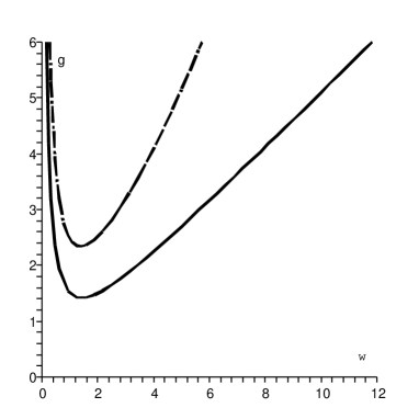
Figure 1. The $\omega$-$g$ curves ($\Sigma$) when $K(x)\equiv 1$, $\beta=-0.5$, for the cases $c=0$, $c=1$ (dashed line).

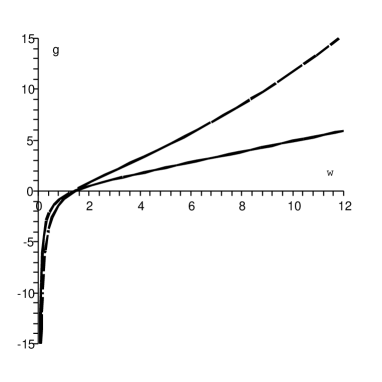
Figure 2. The $\omega$-$g$ curves ($\Sigma$) when $K(x)\equiv 1$, $\beta=0.5$, for the cases $c=0$, $c=1$ (dashed line).

5. Rotating waves on a ring in the general case

We now return to the case when $K\in L^{\infty}(\mathbb{R})$ is a function satisfying (15),(16) (these will be standing assumptions throughout this section and the next one), and prove that several of the results about rotating waves obtained above for the special case of uniform coupling remain valid, though the proofs are necessarily less direct.

Our main theorem generalizes the representation (79) for $\Sigma$ which was obtained in the case of uniform coupling. The function $f_{c,\beta}(\omega)$ will be replaced by a function $g(\omega)$, for which, unlike in the uniform-coupling case, we cannot obtain an explicit expression, but we shall be able to derive some key qualitative properties, which are similar to those of $f_{c,\beta}$.

Theorem 20.

The synaptic-coupling strength ($g$) vs. velocity ($\omega$) curve $\Sigma$, defined by (65) can be represented as the graph of a function:

(97) $$\Sigma=\{(\omega,g(\omega))\;|\;\omega\in(0,\infty)\},$$

where $g:(0,\infty)\rightarrow\mathbb{R}$ is a continuous function and

we have

(98) $$\lim_{\omega\rightarrow+\infty}g(\omega)=+\infty,$$

and

(i) When $\omega^{2}\geq 4\beta$ we have the inequalities:

(99) $$\frac{1}{\overline{K}}f_{c,\beta}(\omega)\leq g(\omega)\leq\frac{1}{\underline{K}}f_{c,\beta}(\omega),$$

(100) $$\frac{2}{\|K\|_{L^{1}[0,2\pi]}}\Big{(}\frac{\omega^{2}}{4}-\beta\Big{)}\Big{(}e^{\frac{c}{2}+\frac{2\pi}{\omega}}-1\Big{)}e^{-\frac{2\pi}{\omega}}\leq g(\omega)\leq\frac{2}{\|K\|_{L^{1}[0,2\pi]}}\Big{(}\frac{\omega^{2}}{4}-\beta\Big{)}\Big{(}e^{\frac{c}{2}+\frac{2\pi}{\omega}}-1\Big{)}.$$

(ii) When $\omega^{2}\leq 4\beta$ we have the inequalities:

(101) $$\frac{1}{\underline{K}}f_{c,\beta}(\omega)\leq g(\omega)\leq\frac{1}{\overline{K}}f_{c,\beta}(\omega),$$

(102) $$\frac{2}{\|K\|_{L^{1}[0,2\pi]}}\Big{(}\frac{\omega^{2}}{4}-\beta\Big{)}\Big{(}e^{\frac{c}{2}+\frac{2\pi}{\omega}}-1\Big{)}\leq g(\omega)\leq\frac{2}{\|K\|_{L^{1}[0,2\pi]}}\Big{(}\frac{\omega^{2}}{4}-\beta\Big{)}\Big{(}e^{\frac{c}{2}+\frac{2\pi}{\omega}}-1\Big{)}e^{-\frac{2\pi}{\omega}}.$$

and

(I) In the excitable case $\beta<0$

$$\lim_{\omega\rightarrow 0+}g(\omega)=+\infty.$$

(II) In the oscillatory case $\beta>0$

$$\lim_{\omega\rightarrow 0+}g(\omega)=-\infty.$$

(III) In the borderline case $\beta=0$

$$\lim_{\omega\rightarrow 0+}g(\omega)=0.$$

Sketching the graphs of $g(\omega)$ as described by theorem 20 in the cases $\beta>0$, $\beta<0$, $\beta=0$, shows that theorem 20 implies theorem 1, and we note that in the case $\beta<0$ we have

(103) $$g_{crit}=\min_{\omega>0}{g(\omega)}.$$

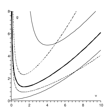
Figure 3. Graph of the function $g(\omega)$ for $K(x)=2+\cos(x),\beta=-0.5,c=1$, obtained numerically (bold curve), together with the graphs of the bounds given by (99) (dashed curves) and by (100) (lighter curves)

.

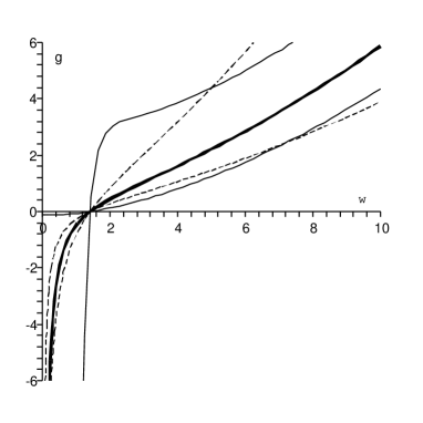
Figure 4. Graph of the function $g(\omega)$ for $K(x)=2+\cos(x),\beta=0.5,c=1$, obtained numerically (bold curve), together with the graphs of the bounds given by (99), (101) (dashed curves) and by (100),(102) (lighter curves)

.

Figure 3 illustrates the contents of theorem 20 in the excitable case. In this example we take $K(x)=2+\cos(x),\beta=-0.5,c=1$. The bold curve shows the graph of the function $g(\omega)$ (or in other words the curve $\Sigma$), obtained by laborious numerical computation: we numerically solved the equation (64) for $g$, with the parameter $\omega$ taking values in the interval $(0,10)$ - using the bisection method. Note that each evaluation of the function $\Psi$ requires numerically solving the initial-value problem (61), (62). The dashed curves in the figure represent the lower and upper bounds on $g(\omega)$ given by (99), while the lighter curves represent the lower and upper bounds given by (100).

Figure 4 illustrates the contents of theorem 20 in the oscillatory case. We take $K(x)=2+\cos(x),\beta=-0.5,c=1$. The bold curve shows the graph of the function $g(\omega)$, obtained numerically, The dashed curves in the figure represent the lower and upper bounds on $g(\omega)$ given by (99),(101) while the lighter curves represent the lower and upper bounds given by (100),(102).

We prove theorem 20 by using the following lemmas, whose proofs will follow.

We define the functions

$$\underline{g}(\omega)=\frac{1}{\overline{R}_{\omega}}\Big{(}\frac{\omega^{2}}{4}-\beta\Big{)},\;\;\;\overline{g}(\omega)=\frac{1}{\underline{R}_{\omega}}\Big{(}\frac{\omega^{2}}{4}-\beta\Big{)}.$$

Lemma 21.

(i) If $\omega^{2}\geq 4\beta$ then

(104) $$0\leq\frac{1}{\overline{K}}f_{c,\beta}(\omega)\leq\underline{g}(\omega)\leq\overline{g}(\omega)\leq\frac{1}{\underline{K}}f_{c,\beta}(\omega),$$

(105) $$\frac{2}{\|K\|_{L^{1}[0,2\pi]}}\Big{(}\frac{\omega^{2}}{4}-\beta\Big{)}\Big{(}e^{\frac{c}{2}+\frac{2\pi}{\omega}}-1\Big{)}e^{-\frac{2\pi}{\omega}}\leq\underline{g}(\omega)\leq\overline{g}(\omega)\leq\frac{2}{\|K\|_{L^{1}[0,2\pi]}}\Big{(}\frac{\omega^{2}}{4}-\beta\Big{)}\Big{(}e^{\frac{c}{2}+\frac{2\pi}{\omega}}-1\Big{)}.$$

(ii) If $\omega^{2}\leq 4\beta$ then

(106) $$\frac{1}{\underline{K}}f_{c,\beta}(\omega)\leq\overline{g}(\omega)\leq\underline{g}(\omega)\leq\frac{1}{\overline{K}}f_{c,\beta}(\omega)\leq 0,$$

(107) $$\frac{2}{\|K\|_{L^{1}[0,2\pi]}}\Big{(}\frac{\omega^{2}}{4}-\beta\Big{)}\Big{(}e^{\frac{c}{2}+\frac{2\pi}{\omega}}-1\Big{)}\leq\underline{g}(\omega)\leq\frac{2}{\|K\|_{L^{1}[0,2\pi]}}\Big{(}\frac{\omega^{2}}{4}-\beta\Big{)}\Big{(}e^{\frac{c}{2}+\frac{2\pi}{\omega}}-1\Big{)}e^{-\frac{2\pi}{\omega}}.$$

Lemma 22.

If either

(i) $g\geq 0$ and $g<\underline{g}(\omega)$

or

(ii) $g\leq 0$ and $g<\overline{g}(\omega)$

then

(108) $$\Psi(\omega,g)<1.$$

Lemma 23.

If either

(i) $g\geq 0$ and $g>\overline{g}(\omega)$.

or

(ii) $g\leq 0$ and $g>\underline{g}(\omega)$.

then

(109) $$\Psi(\omega,g)>1.$$

Lemma 24.

Fixing $\omega>0$, there is at most one value of $g$ for which (64) holds.

Using the above lemmas, we can give the

proof of theorem 20: First we fix $\omega>0$ satisfying $\omega^{2}\geq 4\beta$. Then by part (i) of lemma 21 we have $0\leq\underline{g}(\omega)\leq\overline{g}(\omega)$, hence by part (i) of lemma 22, part (i) of lemma 23 and the intermediate-value theorem, there exists $g$ satisfying $\underline{g}(\omega)\leq g\leq\overline{g}(\omega)$ with $\Psi(\omega,g)=1$. By lemma 24 this $g$ is unique, so we may denote it by $g(\omega)$.

Now fix $\omega>0$ satisfying $\omega^{2}\leq 4\beta$. Then by part (ii) of lemma 21 we have $\overline{g}(\omega)\leq\underline{g}(\omega)\leq 0$, hence by part (ii) of lemma 22, part (ii) of lemma 23 and the intermediate-value theorem, there exists $g$ satisfying $\overline{g}(\omega)\leq g\leq\underline{g}(\omega)$ with $\Psi(\omega,g)=1$. By lemma (24) this $g$ is unique, so we may denote it by $g(\omega)$.

We have thus proven the existence of $g(\omega)$ satisfying (97), and

(110) $$\omega^{2}\geq 4\beta\;\Rightarrow 0\leq\underline{g}(\omega)\leq g(\omega)\leq\overline{g}(\omega).$$

(111) $$\omega^{2}\leq 4\beta\;\Rightarrow\overline{g}(\omega)\leq g(\omega)\leq\underline{g}(\omega)\leq 0.$$

Parts (i),(ii) of theorem 20 follow from (110),(111) and lemma 21.

(98) follows from part (i) of the theorem, and (80).

Parts (I)-(III) of theorem 20 follow from (99) and (101), along with (81), (82) and (83).

To conclude the proof of theorem 20 we only need to show that $g(\omega)$ is continuous, but this follows at once from (97), since by continuity of $\Psi$, the set $\Sigma$ is closed, and this set is the graph of $g(\omega)$.

We now turn to the proofs of lemmas 21-24.

Lemma 21 is an immediate consequence of the definitions of $\underline{g}(\omega)$,$\overline{g}(\omega)$ and of the inequalities of lemmas 13 and 14.

We now start working towards proving lemma 22.

Lemma 25.

If either

(i) $g\geq 0$ and

(112) $$\beta+g\overline{R}_{\omega}<0$$

or

(ii) $g\leq 0$ and

(113) $$\beta+g\underline{R}_{\omega}<0$$

then

$$\Psi(\omega,g)<\frac{2}{3}.$$

proof: (i) We will show that when (112) holds we have

(114) $$\phi_{\omega,g}(z)<2\pi\;\;\;\forall z\geq 0,$$

which, together with (63), implies the result of our lemma. To prove our claim we note that, using (61),(26),(28),(112), and the assumption that $g\geq 0$

(115) $$\phi_{\omega,g}(z)=2\pi\; \Rightarrow\; \phi_{\omega,g}^{\prime}(z)=\frac{2}{\omega}[\beta+gR_{\omega}(z)]$$

$$\leq \frac{2}{\omega}[\beta+g\overline{R}_{\omega}]<0.$$

We now show that (115) implies (114). If (114) fails to hold, then we set

$$z_{0}=\min\;\{z\geq 0\;|\;\phi_{\omega,g}(z)=2\pi\}.$$

This number is well-defined by continuity and by the fact that $\phi_{\omega,g}(0)=\pi$, which implies also that $z_{0}>0$. By (115) we have $\phi_{\omega,g}^{\prime}(z_{0})<0$, but this implies that $\phi_{\omega,g}(z)$ is decreasing in a neighborhood of $z_{0}$, and in particular that there exist $z\in(0,z_{0})$ satisfying $\phi_{\omega,g}(z)=2\pi.$ But this contradicts the definition of $z_{0}$, and this contradiction proves (114).

(ii) In the case that $g\leq 0$ and (113) holds, we replace (115) with

$$\phi_{\omega,g}(z)=2\pi\; \Rightarrow\; \phi_{\omega,g}^{\prime}(z)=\frac{2}{\omega}[\beta+gR_{\omega}(z)]$$

$$\leq \frac{2}{\omega}[\beta+g\underline{R}_{\omega}]<0.$$

so that the proof proceeds as before.

proof of lemma 22: (i) We assume that $g\geq 0$ and $g<\underline{g}(\omega)$, i.e.

(116) $$g<\frac{1}{\overline{R}_{\omega}}\Big{(}\frac{\omega^{2}}{4}-\beta\Big{)}$$

and prove (108).

By (63), (108) is equivalent to

(117) $$\phi_{\omega,g}(2\pi)<3\pi.$$

We note that, by part (i) of lemma 25, we already have (108) when (112) holds, hence we may assume

(118) $$\overline{\mu}=\beta+g\overline{R}_{\omega}\geq 0.$$

Using (61) and the assumption that $g\geq 0$, we have

(119) $$\phi_{\omega,g}^{\prime}(z) = \frac{1}{\omega}[h(\phi_{\omega,g}(z))+gR_{\omega}(z)w(\phi_{\omega,g}(z))]$$

$$\leq \frac{1}{\omega}\Big{[}1-\cos(\phi_{\omega,g}(z))+\Big{(}\beta+g\overline{R}_{\omega}\Big{)}(1+\cos(\phi_{\omega,g}(z)))\Big{]}$$

$$= \frac{1}{\omega}[(\overline{\mu}+1)+(\overline{\mu}-1)\cos(\phi_{\omega,g}(z))].$$

which implies (note that the integral below is well-defined because $\overline{\mu}\geq 0$ - if $\overline{\mu}=0$ the integral is infinite)

$$\int_{0}^{2\pi}{\frac{\phi_{\omega,g}^{\prime}(z)dz}{(\overline{\mu}+1)+(\overline{\mu}-1)\cos(\phi_{\omega,g}(z))}}\leq\frac{2\pi}{\omega}.$$

Making the change of variables $\varphi=\phi_{\omega,g}(z)$ we obtain

(120) $$\int_{\phi_{\omega,g}(0)}^{\phi_{\omega,g}(2\pi)}{\frac{d\varphi}{(\overline{\mu}+1)+(\overline{\mu}-1)\cos(\varphi)}}\leq\frac{2\pi}{\omega}.$$

If we assume, by way of contradiction, that (117) does not hold, i.e. that $\phi_{\omega,g}(2\pi)\geq 3\pi$, then, using (75),

$$\int_{\phi_{\omega,g}(0)}^{\phi_{\omega,g}(2\pi)}{\frac{d\varphi}{(\overline{\mu}+1)+(\overline{\mu}-1)\cos(\varphi)}}\geq\int_{\pi}^{3\pi}{\frac{d\varphi}{(\overline{\mu}+1)+(\overline{\mu}-1)\cos(\varphi)}}=\frac{\pi}{\sqrt{\overline{\mu}}},$$

so together with (120) we obtain

$$\frac{1}{\sqrt{\overline{\mu}}}\leq\frac{2}{\omega},$$

which is equivalent to

$$g\geq\frac{1}{\overline{R}_{\omega}}\Big{(}\frac{\omega^{2}}{4}-\beta\Big{)},$$

which contradicts (116). This contradiction proves (117), concluding the proof that (i) implies (108).

(ii) We assume that $g\leq 0$ and $g<\overline{g}(\omega)$, i.e.

(121) $$g<\frac{1}{\underline{R}_{\omega}}\Big{(}\frac{\omega^{2}}{4}-\beta\Big{)}$$

and prove (117).

We note that, by part (ii) of lemma 25, we already have (108) when (113) holds, hence we may assume

$$\underline{\mu}=\beta+g\underline{R}_{\omega}\geq 0.$$

We now replace (119) by

$$\phi_{\omega,g}^{\prime}(z) = \frac{1}{\omega}[h(\phi_{\omega,g}(z))+gR_{\omega}(z)w(\phi_{\omega,g}(z))]$$

$$\leq \frac{1}{\omega}\Big{[}1-\cos(\phi_{\omega,g}(z))+\Big{(}\beta+g\underline{R}_{\omega}\Big{)}(1+\cos(\phi_{\omega,g}(z)))\Big{]}$$

$$= \frac{1}{\omega}[(\underline{\mu}+1)+(\underline{\mu}-1)\cos(\phi_{\omega,g}(z))].$$

The proof then proceeds as before.

proof of lemma 23: (i) We assume $g\geq 0$ and $g>\overline{g}(\omega)$, i.e.,

(122) $$g>\frac{1}{\underline{R}_{\omega}}\Big{(}\frac{\omega^{2}}{4}-\beta\Big{)}$$

and prove that $\Psi(\omega,g)>1$. By (63), our claim is equivalent to

(123) $$\phi_{\omega,g}(2\pi)>3\pi.$$

We define

$$\underline{\mu}=\beta+g\underline{R}_{\omega},$$

and we note that (122) is equivalent to

(124) $$\underline{\mu}>\frac{\omega^{2}}{4}.$$

Using (61) and $g\geq 0$ we have

(125) $$\phi_{\omega,g}^{\prime}(z) = \frac{1}{\omega}[h(\phi_{\omega,g}(z))+gR_{\omega}(z)w(\phi_{\omega,g}(z))]$$

$$\geq \frac{1}{\omega}\Big{[}1-\cos(\phi_{\omega,g}(x))+\Big{(}\beta+g\underline{R}_{\omega}\Big{)}(1+\cos(\phi_{\omega,g}(z)))\Big{]}$$

$$= \frac{1}{\omega}[(\underline{\mu}+1)+(\underline{\mu}-1)\cos(\phi_{\omega,g}(z))],$$

which implies

$$\int_{\pi}^{3\pi}{\frac{\phi_{\omega,g}^{\prime}(z)dz}{(\underline{\mu}+1)+(\underline{\mu}-1)\cos(\phi_{\omega,g}(z))}}\geq\frac{2\pi}{\omega}.$$

Making the change of variables $\varphi=\phi_{\omega,g}(z)$, we obtain

(126) $$\int_{\phi_{\omega,g}(0)}^{\phi_{\omega,g}(2\pi)}{\frac{d\varphi}{(\underline{\mu}+1)+(\underline{\mu}-1)\cos(\varphi)}}\geq\frac{2\pi}{\omega}.$$

If we assume, by way of contradiction, that (123) does not hold, i.e. that $\phi_{\omega,g}(2\pi)\leq 3\pi$, then, using (75),

$$\int_{\phi_{\omega,g}(0)}^{\phi_{\omega,g}(2\pi)}{\frac{d\varphi}{(\underline{\mu}+1)+(\underline{\mu}-1)\cos(\varphi)}}\leq\int_{\pi}^{3\pi}{\frac{d\varphi}{(\underline{\mu}+1)+(\underline{\mu}-1)\cos(\varphi)}}=\frac{\pi}{\sqrt{\underline{\mu}}},$$

so together with (126) we obtain

$$\frac{1}{\sqrt{\underline{\mu}}}\geq\frac{2}{\omega}.$$

This contradicts (124), and this contradiction implies that (123) holds, completing our proof that (i) implies (109).

(ii) We assume $g\leq 0$ and $g>\underline{g}(\omega)$, i.e.,

(127) $$g>\frac{1}{\overline{R}_{\omega}}\Big{(}\frac{\omega^{2}}{4}-\beta\Big{)}$$

and prove (109). We define

$$\overline{\mu}=\beta+g\overline{R}_{\omega},$$

and we note that (127) is equivalent to

$$\overline{\mu}>\frac{\omega^{2}}{4}.$$

Using (61) and $g\leq 0$ we have

$$\phi_{\omega,g}^{\prime}(z) = \frac{1}{\omega}[h(\phi_{\omega,g}(z))+gR_{\omega}(z)w(\phi_{\omega,g}(z))]$$

$$\geq \frac{1}{\omega}\Big{[}1-\cos(\phi_{\omega,g}(x))+\Big{(}\beta+g\overline{R}_{\omega}\Big{)}(1+\cos(\phi_{\omega,g}(z)))\Big{]}$$

$$= \frac{1}{\omega}[(\overline{\mu}+1)+(\overline{\mu}-1)\cos(\phi_{\omega,g}(z))],$$

and the rest of the proof proceeds as in case (i) above.

To prove lemma 24 we shall prove the following more general lemma - from which lemma 24 follows by setting $R(z)=R_{\omega}(z)$, and which we shall also have occasion to use once more later.

Lemma 26.

Consider the differential equation

(128) $$\phi^{\prime}(z)=\frac{1}{\omega}[h(\phi(z))+gR(z)w(\phi(z))]$$

where $h$,$w$ are defined by (10), $\omega>0$ is fixed, and $R\in C^{2}[0,2\pi]$ is a positive function. Then there exists at most one value of $g$ for which the boundary-value problem (128) and

(129) $$\phi(0)=\pi,\;\;\phi(2\pi)=3\pi$$

has a solution.

proof: Assume by way of contradiction that $g_{2}>g_{1}$ and $\phi_{1}(z)$ and $\phi_{2}(z)$ satisfy the differential equations

(130) $$\phi_{1}^{\prime}(z)=\frac{1}{\omega}[h(\phi_{1}(z))+g_{1}R(z)w(\phi_{1}(z))],$$

(131) $$\phi_{2}^{\prime}(z)=\frac{1}{\omega}[h(\phi_{2}(z))+g_{2}R(z)w(\phi_{2}(z))],$$

with boundary conditions

(132) $$\phi_{1}(0)=\phi_{2}(0)=\pi.$$

(133) $$\phi_{1}(2\pi)=\phi_{2}(2\pi)=3\pi.$$

We define

$$\varphi(z)=\phi_{2}(z)-\phi_{1}(z).$$

From (132) and (133) we have

(134) $$\varphi(0)=\varphi(2\pi)=0.$$

We now compute the first three derivatives of $\varphi(z)$ at $z=0,2\pi$. We shall be using (25), (27), as well as the facts that

$$h^{\prime}((2l+1)\pi)=0,\;\;w^{\prime}((2l+1)\pi)=0\;\;\;\forall l\in\mathbb{Z},$$

$$h^{\prime\prime}((2l+1)\pi)=\beta-1,\;\;w^{\prime\prime}((2l+1)\pi)=1\;\;\;\forall l\in\mathbb{Z}.$$

Substituting $z=0,2\pi$ into (130),(131) and using (132), (133) we have

(135) $$\phi_{1}^{\prime}(0)=\phi_{2}^{\prime}(0)=\phi_{1}^{\prime}(2\pi)=\phi_{2}^{\prime}(2\pi)=\frac{2}{\omega},$$

hence

(136) $$\varphi^{\prime}(0)=\varphi^{\prime}(2\pi)=0.$$

Differentiating (128) we have

(137) $$\phi^{\prime\prime}(z)=\frac{1}{\omega}[h^{\prime}(\phi(z))\phi^{\prime}(z)+gR^{\prime}(z)w(\phi(z))+gR(z)w^{\prime}(\phi(z))\phi^{\prime}(z)],$$

and substituting $z=0,2\pi$ into (137) and using (132),(133) and (135) we obtain

(138) $$\phi_{1}^{\prime\prime}(0)=\phi_{2}^{\prime\prime}(0)=\phi_{1}^{\prime\prime}(2\pi)=\phi_{2}^{\prime\prime}(2\pi)=0,$$

So that

(139) $$\varphi^{\prime\prime}(0)=\varphi^{\prime\prime}(2\pi)=0.$$

Differentiating (137) we have

(140) $$\phi^{\prime\prime\prime}(z) = \frac{1}{\omega}[h^{\prime\prime}(\phi(z))(\phi^{\prime}(z))^{2}+h^{\prime}(\phi(z))\phi^{\prime\prime}_{\omega,g}(z)$$

$$+ gR^{\prime\prime}(z)w(\phi(z))+2gR^{\prime}(z)w^{\prime}(\phi(z))\phi^{\prime}(z)$$

$$+ gR(z)w^{\prime\prime}(\phi(z))(\phi^{\prime}(z))^{2}+gR(z)w^{\prime}(\phi(z))\phi^{\prime\prime}(z)],$$

and upon substituting $z=0,2\pi$ into (140) and using (132), (133), (135) and (138) we obtain

$$\phi_{1}^{\prime\prime\prime}(0)=\frac{4}{\omega^{3}}(\beta-1+g_{1}R(0)),\;\;\phi_{2}^{\prime\prime\prime}(0)=\frac{4}{\omega^{3}}(\beta-1+g_{2}R(0))$$

$$\phi_{1}^{\prime\prime\prime}(2\pi)=\frac{4}{\omega^{3}}(\beta-1+g_{1}R(2\pi)),\;\;\phi_{2}^{\prime\prime\prime}(2\pi)=\frac{4}{\omega^{3}}(\beta-1+g_{2}R(2\pi))$$

hence, using also the assumption that $g_{2}>g_{1}$,

(141) $$\varphi^{\prime\prime\prime}(0)=\frac{4}{\omega^{3}}(g_{2}-g_{1})R(0)>0.$$

(142) $$\varphi^{\prime\prime\prime}(2\pi)=\frac{4}{\omega^{3}}(g_{2}-g_{1})R(2\pi)>0.$$

From (134),(136),(139), (141) and (142) we conclude that there exists $\epsilon>0$ such that

(143) $$z\in[0,\epsilon]\;\;\Rightarrow\;\;\varphi(z)>0$$

(144) $$z\in[2\pi-\epsilon,2\pi]\;\;\Rightarrow\;\;\varphi(z)<0.$$

We will now use (143),(144) to derive a contradiction. First note that if $z_{0}\in(0,2\pi)$ and $\varphi(z_{0})=0$, then using the definition of $\varphi(z)$ and lemma 15 we have

$$\pi<\phi_{2}(z_{0})=\phi_{1}(z_{0})<3\pi,$$

which implies

$$h(\phi_{1}(z_{0}))=h(\phi_{2}(z_{0})),$$

$$w(\phi_{1}(z_{0}))=w(\phi_{2}(z_{0}))>0,$$

which together with (130),(131) and the assumption that $g_{2}>g_{1}$ imply

$$\phi_{2}^{\prime}(z_{0})>\phi_{1}^{\prime}(z_{0}),$$

or in other words that

$$\varphi^{\prime}(z_{0})>0.$$

We have thus shown that

(145) $$z\in(0,2\pi),\;\;\varphi(z)=0\;\;\Rightarrow\varphi^{\prime}(z)>0.$$

Let

$$z_{1}=\inf\{z\in(0,2\pi)\;|\;\varphi(z)<0\}$$

(note that by (144) the above set is nonempty, and by (143) it is bounded from below. By (143) we have $z_{1}>0$ and by continuity we have $\varphi(z_{1})=0$. Hence by (145) we have $\varphi^{\prime}(z_{1})>0$. But this implies that for $z<z_{1}$ sufficiently close to $z_{1}$ we have $\varphi(z)<0$, contradicting the definition of $z_{1}$. This contradiction establishes the lemma.

Question 27.

We have shown that several of the qualitative features that we derived by direct computation in the case of uniform coupling (section 4) remain valid in the general case. It is natural to ask whether more can be said, e.g., whether for any $K(x)$, when $\beta<0$ and $g>g_{crit}$ there exist precisely two rotating waves. This would follow if we could prove that the only local minimum of the function $g(\omega)$ is the global one. However, as we show by numerical computations in section 9, there are in fact cases in which the function $g(\omega)$ has two minima, and values of $g$ for which four rotating waves exist. Thus a modified conjecture is that for sufficiently large $g$ there are exactly two rotating waves.

Question 28.

Is it true that in the oscillatory case $\beta\geq 0$ the rotating wave is always unique? In section 4 we saw that this is the case when $K(x)$ is constant. This would follow if we could show that $g(\omega)$ is an increasing function.

6. Some quantitative bounds

Based on the results of the previous section, we now obtain some explicit bounds for the velocities of the rotating waves and, in the excitable case, for the critical synaptic-coupling strength $g_{crit}$.

We first note that the inequalities (100) imply that when $c>0$

(146) $$g_{k}(\omega)=\frac{1}{2\|K\|_{L^{1}[0,2\pi]}}(e^{\frac{c}{2}}-1)\omega^{2}+O(\omega)\;\;\;as\;\;\omega\rightarrow+\infty,$$

while when $c=0$

(147) $$g_{k}(\omega)=\frac{\pi}{\|K\|_{L^{1}[0,2\pi]}}\omega+O(1)\;\;\;as\;\;\omega\rightarrow+\infty.$$

These asymptotic expressions imply asymptotic expressions for the velocity $\omega$ in the case $g\rightarrow\infty$ in the case $\beta\geq 0$, and for the velocity of the fast wave in the case $\beta<0$.

Theorem 29.

(I) In the excitable case $\beta<0$, when $c>0$, the velocity $\omega_{f}$ of the fast rotating wave satisfies

(148) $$\omega_{f}=\sqrt{\frac{2\|K\|_{L^{1}[0,2\pi]}}{e^{\frac{c}{2}}-1}}\sqrt{g}+O(1)\;\;\;as\;\;g\rightarrow+\infty,$$

while in the case $c=0$

(149) $$\omega_{f}=\frac{\|K\|_{L^{1}[0,2\pi]}}{\pi}g+O(1)\;\;\;as\;\;g\rightarrow+\infty,$$

(II) In the case $\beta\geq 0$ we have the same asymptotic formulas (148), (149) for the velocity of the rotating wave $\omega$.

By using the inequalities in (99),(101) and lemmas 17 and 18 we can obtain explicit bounds on the velocities of both the slow and fast rotating waves in terms of the functions $\omega_{c,\beta}$,$\underline{\omega}_{c,\beta}$,$\overline{\omega}_{c,\beta}$ defined by lemma 17, as well as simple asymptotic bounds for the velocity of the slow wave as $g\rightarrow+\infty$ in the case $\beta<0$ (note that theorem 29 above has already provided us with asymptotics for the fast wave), and for the velocity as $g\rightarrow-\infty$ in the case $\beta>0$.

Theorem 30.

(I) In the excitable case $\beta<0$, assume $g>\frac{\Omega(c,\beta)}{\underline{K}}$. Then there exist a ‘slow’ rotating wave with velocity $\omega_{s}$ bounded from above by

(150) $$\underline{\omega}_{c,\beta}\Big{(}\overline{K}g\Big{)}\leq\omega_{s}\leq\underline{\omega}_{c,\beta}\Big{(}\underline{K}g\Big{)}$$

and a ‘fast’ rotating wave with velocity $\omega_{f}$ bounded from below by

(151) $$\overline{\omega}_{c,\beta}\Big{(}\underline{K}g\Big{)}\leq\omega_{f}\leq\overline{\omega}_{c,\beta}\Big{(}\overline{K}g\Big{)},$$

where $\underline{\omega}_{c,\beta},\overline{\omega}_{c,\beta}$ are the functions defined by lemma 17.

As a consequence of (150) we have, for the slow wave

(152) $$\frac{2|\beta|e^{\frac{c}{2}}}{\overline{K}}\frac{1}{g}+O\Big{(}\frac{1}{g^{3}}\Big{)}\leq\omega_{s}\leq\frac{2|\beta|e^{\frac{c}{2}}}{\underline{K}}\frac{1}{g}+O\Big{(}\frac{1}{g^{3}}\Big{)}\;\;\;as\;\;g\rightarrow\infty.$$

(II) In the oscillatory case $\beta>0$, there exists a rotating wave solution for any value of $g\in\mathbb{R}$, with velocity $\omega$ bounded by

(153) $$\omega_{c,\beta}(\overline{K}g)\leq\omega\leq\omega_{c,\beta}(\underline{K}g)\;\;\;for\;g\leq 0,$$

(154) $$\omega_{c,\beta}(\underline{K}g)\leq\omega\leq\omega_{c,\beta}(\overline{K}g)\;\;\;for\;g\geq 0,$$

and we have the asymptotic inequalities

(155) $$-\frac{4\beta e^{\frac{c}{2}}}{\overline{K}}\frac{1}{g}+O\Big{(}\frac{1}{g^{3}}\Big{)}\leq\omega\leq-\frac{4\beta e^{\frac{c}{2}}}{\underline{K}}\frac{1}{g}+O\Big{(}\frac{1}{g^{3}}\Big{)}\;\;\;as\;\;g\rightarrow-\infty.$$

(III) In the borderline case $\beta=0$, there exists a rotating wave solution for any value of $g>0$, with velocity $\omega$ bounded as in (154), and

$$\omega=o(1)\;\;\;as\;\;g\rightarrow 0.$$

We now derive explicit lower and upper bounds for the value of $g_{crit}$ in the excitable case $\beta<0$, that is the critical value of $g$ at which two rotating waves are born. Using (103) and (99) we obtain

$$g_{crit}=\min_{\omega>0}g(\omega)\geq\frac{1}{\overline{K}}\min_{\omega>0}f_{c,\beta}(\omega)=\frac{1}{\overline{K}}\Omega(c,\beta)$$

and

$$g_{crit}=\min_{\omega>0}g(\omega)\leq\frac{1}{\underline{K}}\min_{\omega>0}f_{c,\beta}(\omega)=\frac{1}{\underline{K}}\Omega(c,\beta),$$

so that

Lemma 31.

In the excitable case $\beta<0$

$$\frac{1}{\overline{K}}\Omega(c,\beta)\leq g_{crit}\leq\frac{1}{\underline{K}}\Omega(c,\beta).$$

If, instead of using the inequality (99) we use (100), we obtain

Lemma 32.

In the excitable case $\beta<0$

$$\frac{2}{\|K\|_{L^{1}[0,2\pi]}}\min_{\omega\geq 0}\Big{(}\frac{\omega^{2}}{4}-\beta\Big{)}\Big{(}e^{\frac{c}{2}+\frac{2\pi}{\omega}}-1\Big{)}e^{-\frac{2\pi}{\omega}}\leq g_{crit}\leq\frac{2}{\|K\|_{L^{1}[0,2\pi]}}\min_{\omega\geq 0}\Big{(}\frac{\omega^{2}}{4}-\beta\Big{)}\Big{(}e^{\frac{c}{2}+\frac{2\pi}{\omega}}-1\Big{)}$$

7. Periodic travelling waves on the line

We now exploit the results about rotating waves on a ring obtained in the previous sections in order to derive results about periodic waves on the line. As we have already noted in the introduction, periodic waves with wave-number $k$ are the same as rotating waves on the ring with $K=J_{k}$, where $J_{k}$ is defined by (12). We define the function

(156) $$R_{\omega,k}(z)=\int_{0}^{2\pi}{J_{k}(z-y)r_{\omega}(y)dy}$$

as in (58) (with $K=J_{k}$), and similarly the quantities

$$\overline{R}_{\omega,k}(z)=\sup_{x\in\mathbb{R}}{R_{\omega,k}(x)},\;\;\;\underline{R}_{\omega,k}=\inf_{x\in\mathbb{R}}{R_{\omega,k}(x)}$$

as in (66),

$$\overline{J}_{k}=\sup_{x\in\mathbb{R}}{J_{k}(x)},\;\;\underline{J}_{k}=\inf_{x\in\mathbb{R}}{J_{k}(x)}$$

as in (67), and

$$\|J_{k}\|_{L^{1}[0,2\pi]}=\int_{0}^{2\pi}{J_{k}(x)dx}$$

as in (68).

We note that by the definition (12) of $J_{k}$ we have

(157) $$\|J_{k}\|_{L^{1}[0,2\pi]}=\int_{-\infty}^{\infty}{J(z)dz}=\|J\|_{L^{1}(\mathbb{R})}.$$

For each $\omega>0$, $k>0$, $g>0$ we define by $\phi_{\omega,g,k}(z)$ the solution of the initial value problem

(158) $$\phi_{\omega,g,k}^{\prime}(z)=\frac{1}{\omega}[h(\phi_{\omega,g,k}(z))+gR_{\omega,k}(z)w(\phi_{\omega,g,k}(z))],$$

(159) $$\phi_{\omega,g,k}(0)=\pi,$$

the function $\Psi_{k}(\omega,g)$ by

(160) $$\Psi_{k}(\omega,g)=\frac{1}{3\pi}\phi_{\omega,g,k}(2\pi),$$

and the frequency vs. synaptic-coupling strength curve for waves of wave-number $k$ by

(161) $$\Sigma_{k}=\{(\omega,g)\;|\;\Psi_{k}(\omega,g)=1\}.$$

In order to apply theorem 20 to $K=J_{k}$, we need a condition ensuring that $J_{k}\in L^{\infty}(\mathbb{R})$. Such a condition is given by the following

Lemma 33.

Assume $J$ satisfies (22). Then we have

$$|J_{k}(z)-\frac{1}{2\pi}\int_{-\infty}^{\infty}{J(x)dx}|\leq\frac{1}{k}\|J^{\prime}\|_{L^{1}(\mathbb{R})}\;\;\;\forall k>0,z\in\mathbb{R}.$$

In particular $J_{k}\in L^{\infty}(\mathbb{R})$.

proof: We have

$$J_{k}^{\prime}(x)=\frac{1}{k^{2}}\sum_{l=-\infty}^{\infty}{J^{\prime}\Big{(}\frac{1}{k}(x-2\pi l)\Big{)}},$$

hence

(162) $$\|J_{k}^{\prime}\|_{L^{1}[0,2\pi]} = \int_{0}^{2\pi}{|J_{k}^{\prime}(x)|dx}\leq\frac{1}{k^{2}}\sum_{l=-\infty}^{\infty}{\int_{0}^{2\pi}{|J^{\prime}\Big{(}\frac{1}{k}(x-2\pi l)\Big{)}|dx}}$$

$$= \frac{1}{k^{2}}\int_{-\infty}^{\infty}{|J^{\prime}\Big{(}\frac{x}{k}\Big{)}|dx}=\frac{1}{k}\int_{-\infty}^{\infty}{|J^{\prime}(x)|dx}=\frac{1}{k}\|J^{\prime}\|_{L^{1}(\mathbb{R})}.$$

We have, for all $y,z\in[0,2\pi]$

$$|J_{k}(z)-J_{k}(y)|=|\int_{y}^{z}{J_{k}^{\prime}(x)dx}|\leq\int_{0}^{2\pi}{|J_{k}^{\prime}(x)|dx}=\|J_{k}^{\prime}\|_{L^{1}[0,2\pi]}.$$

By periodicity of $J_{k}$ this inequality in fact holds for all $y,z\in\mathbb{R}$, and it implies

$$|J_{k}(z)-\frac{1}{2\pi}\int_{0}^{2\pi}{J_{k}(x)dx}|\leq\|J_{k}^{\prime}\|_{L^{1}[0,2\pi]}\;\;\;\forall x\in\mathbb{R}.$$

Together with the equality (157) and (162), this gives the result of our lemma.

From theorem 20 we thus obtain

Theorem 34.

Assume $J$ satisfies (22) and (23). Then, for each $k>0$, the curve $\Sigma_{k}$ defined by (161) can be represented as the graph of a function:

(163) $$\Sigma_{k}=\{(\omega,g_{k}(\omega))\;|\;\omega\in(0,\infty)\},$$

where $g_{k}:(0,\infty)\rightarrow\mathbb{R}$ is a continuous function which satisfies

(i) When $\omega^{2}\geq 4\beta$:

(164) $$\frac{1}{\overline{J}_{k}}f_{c,\beta}(\omega)\leq g_{k}(\omega)\leq\frac{1}{\underline{J}_{k}}f_{c,\beta}(\omega),$$

(165) $$\frac{2}{\|J\|_{L^{1}(\mathbb{R})}}\Big{(}\frac{\omega^{2}}{4}-\beta\Big{)}\Big{(}e^{\frac{c}{2}+\frac{2\pi}{\omega}}-1\Big{)}e^{-\frac{2\pi}{\omega}}\leq g_{k}(\omega)\leq\frac{2}{\|J\|_{L^{1}(\mathbb{R})}}\Big{(}\frac{\omega^{2}}{4}-\beta\Big{)}\Big{(}e^{\frac{c}{2}+\frac{2\pi}{\omega}}-1\Big{)}.$$

(ii) When $\omega^{2}\leq 4\beta$:

(166) $$\frac{1}{\underline{J}_{k}}f_{c,\beta}(\omega)\leq g_{k}(\omega)\leq\frac{1}{\overline{J}_{k}}f_{c,\beta}(\omega),$$

(167) $$\frac{2}{\|J\|_{L^{1}(\mathbb{R})}}\Big{(}\frac{\omega^{2}}{4}-\beta\Big{)}\Big{(}e^{\frac{c}{2}+\frac{2\pi}{\omega}}-1\Big{)}\leq g_{k}(\omega)\leq\frac{2}{\|J\|_{L^{1}(\mathbb{R})}}\Big{(}\frac{\omega^{2}}{4}-\beta\Big{)}\Big{(}e^{\frac{c}{2}+\frac{2\pi}{\omega}}-1\Big{)}e^{-\frac{2\pi}{\omega}}.$$

and

(I) In the oscillatory case $\beta>0$

(168) $$\lim_{\omega\rightarrow 0+}g_{k}(\omega)=-\infty.$$

(II) In the excitable case $\beta<0$

(169) $$\lim_{\omega\rightarrow 0+}g_{k}(\omega)=+\infty.$$

(III) In the borderline case $\beta=0$

(170) $$\lim_{\omega\rightarrow 0+}g_{k}(\omega)=0.$$

When $\beta<0$, for each $k>0$ we have the critical value

$$g_{crit}(k)=\min_{\omega>0}g_{k}(\omega),$$

above which we have the existence of two periodic travelling waves of wave-number $k$. From lemma 32 we have

Lemma 35.

Assume $J$ satisfies (22) and (23), and $\beta<0$. Then for all $k>0$

$$\frac{2}{\|J\|_{L^{1}(\mathbb{R})}}\min_{\omega\geq 0}\Big{(}\frac{\omega^{2}}{4}-\beta\Big{)}\Big{(}e^{\frac{c}{2}+\frac{2\pi}{\omega}}-1\Big{)}e^{-\frac{2\pi}{\omega}}\leq g_{crit}(k)\leq\frac{2}{\|J\|_{L^{1}(\mathbb{R})}}\min_{\omega\geq 0}\Big{(}\frac{\omega^{2}}{4}-\beta\Big{)}\Big{(}e^{\frac{c}{2}+\frac{2\pi}{\omega}}-1\Big{)}$$

which shows that $g_{crit}(k)$ is bounded between two positive constants for all $k>0$, as claimed in part (II)(B) of theorem 2.

Using theorem 29, the identity (157), and the expression $v=\frac{\omega}{k}$ for the velocity of the periodic travelling waves, we obtain the asymptotic velocity of the periodic travelling wave in the oscillatory case, and of the fast periodic travelling wave in the excitable case for the cse of strong synaptic coupling ($g$).

Theorem 36.

Assume $J$ satisfies (22) and (23). Then, for each $k>0$,

(I) In the excitable case $\beta<0$, when $c>0$, the velocity $v_{f}$ of the fast periodic travelling wave of wave-number $k$ satisfies

(171) $$v_{f}=\frac{1}{k}\sqrt{\frac{2\|J\|_{L^{1}(\mathbb{R})}}{e^{\frac{c}{2}}-1}}\sqrt{g}+O(1)\;\;\;as\;\;g\rightarrow+\infty,$$

while in the case $c=0$

(172) $$v_{f}=\frac{1}{k}\frac{\|J\|_{L^{1}(\mathbb{R})}}{\pi}g+O(1)\;\;\;as\;\;g\rightarrow+\infty,$$

(II) In the case $\beta\geq 0$ we have the same asymptotic formulas (148), (149) for the velocity of the periodic travelling wave of wave-number $k$.

Let us note that the quantitative bounds for the velocities of travelling waves on a ring given in theorem 30, imply bounds for the velocities of periodic travelling waves of wave-number $k$, and asymptotic bounds as $g\rightarrow\infty$ for the velocity of obtained by replacing $\overline{K},\underline{K}$ by $\overline{J}_{k},\underline{J}_{k}$. However in contrast with the result of theorem 36, these bounds depend on the quantities $\overline{J}_{k},\underline{J}_{k}$, so the dependence on $k$ is not as explicit and must be computed for each individual synaptic-coupling kernel $J$.

The curves $\Sigma_{k}$ obviously depend on the shape of the synaptic-coupling kernel $J$. However in the next sections, where we investigate the limits of large and of small wave number, we shall discover that in these limits these curves tend to shapes which are independent of the shape of $J$ (depending on $J$ only through the norm $\|J\|_{L^{1}(\mathbb{R})})$.

8. Periodic travelling waves on the line: large wave-number

This section is devoted to the study of periodic travelling waves with large wave-number $k$. The main point which we shall prove is that although clearly the frequency vs. coupling-strength curve for each finite $k>0$ depends on the details of the coupling-kernel $J$, as $k\rightarrow\infty$ this curve approaches a limiting curve which is independent of details of $J$, depending only (in a trivial way) on the norm $\|J\|_{L^{1}(\mathbb{R})}$, and is thus ‘universal’. Indeed we shall see that the case $k\rightarrow\infty$ is related to the case of uniform coupling on a ring studied in section 4, and thus we will be able to obtain a closed expression for this limiting curve.

From lemma 33 we have

$$\frac{1}{2\pi}\|J\|_{L^{1}(\mathbb{R})}-\frac{1}{k}\|J^{\prime}\|_{L^{1}(\mathbb{R})}\leq\underline{J}_{k}\leq\overline{J}_{k}\leq\frac{1}{2\pi}\|J\|_{L^{1}(\mathbb{R})}+\frac{1}{k}\|J^{\prime}\|_{L^{1}(\mathbb{R})},$$

implying

$$\lim_{k\rightarrow+\infty}{\underline{J}_{k}}=\lim_{k\rightarrow+\infty}{\overline{J}_{k}}=\frac{1}{2\pi}\|J\|_{L^{1}(\mathbb{R})},$$

which, together with (164) and (166) implies

Theorem 37.

Assume $J$ satisfies (22) and (23). We have

$$\lim_{k\rightarrow+\infty}g_{k}(\omega)=g_{\infty}(\omega),$$

where

$$g_{\infty}(\omega)=\frac{2\pi}{\|J\|_{L^{1}(\mathbb{R})}}f_{c,\beta}(\omega)$$

uniformly for $\omega$ in compact subsets of $(0,\infty)$, and if $\beta<0$

$$\lim_{k\rightarrow+\infty}g_{crit}(k)=\frac{2\pi}{\|J\|_{L^{1}(\mathbb{R})}}\Omega(c,\beta).$$

This implies

Theorem 38.

Assume $J$ satisfies (22) and (23). Then

(I) In the oscillatory case $\beta>0$, for any $g\in\mathbb{R}$ and $k>0$ we have: there exists a periodic travelling wave with wave-number $k$, and its frequency satisfies

(173) $$\lim_{k\rightarrow\infty}{\omega(k)}=\omega_{c,\beta}\Big{(}\frac{g}{2\pi}\|J\|_{L^{1}(\mathbb{R})}\Big{)},$$

where $\omega_{c,\beta}$ is given by lemma 17.

(II) In the excitable case $\beta<0$:

(i) If $g<\frac{2\pi}{\|J\|_{L^{1}(\mathbb{R})}}\Omega(c,\beta)$ then for $k$ sufficiently large there are no periodic travelling waves with wave-number $k$.

(ii) If $g>\frac{2\pi}{\|J\|_{L^{1}(\mathbb{R})}}\Omega(c,\beta)$ then for $k$ sufficiently large there are two periodic travelling waves with wave-number $k$, and their frequencies $\omega_{s}(k)$, $\omega_{f}(k)$ satisfy

$$\lim_{k\rightarrow\infty}{\omega_{s}(k)}=\underline{\omega}_{c,\beta}\Big{(}\frac{g}{2\pi}\|J\|_{L^{1}(\mathbb{R})}\Big{)},\;\;\;\lim_{k\rightarrow\infty}{\omega_{f}(k)}=\overline{\omega}_{c,\beta}\Big{(}\frac{g}{2\pi}\|J\|_{L^{1}(\mathbb{R})}\Big{)},$$

where the functions $\underline{\omega}_{c,\beta},\overline{\omega}_{c,\beta}$ are given by lemma 17.

(III) In the boundary case $\beta=0$:

(i) For any $g>0$ we have: for any $k>0$ there exists a periodic travelling wave with wave-number $k$, and its frequency satisfies (173).

(ii) For any $g\leq 0$ there are no periodic travelling waves.

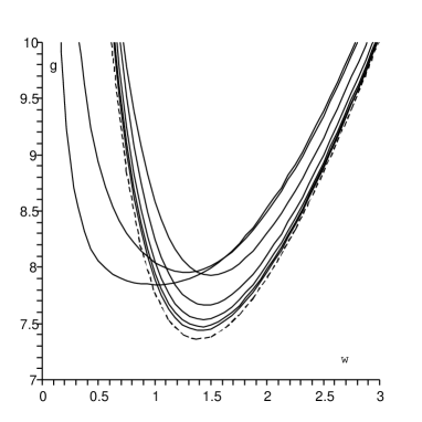
Figure 5. Graphs of the functions $g_{k}(\omega)$ for $k=0.25,0.5,1.5,2.5,3.5,4.5,5.5$, and the graph of the function $g_{\infty}(\omega)$ (dashed), in the case $\beta=-0.5$,$c=1$ obtained numerically.

We now present the results of some numerical computations which we carried out, and these will demonstrate the results of theorem 37. For our computations we chose

$$J(x)=e^{-|x|},$$

so that $\|J\|_{L^{1}(\mathbb{R})}=2$ and a calculation shows that

$$J_{k}(z)=\frac{1}{k}\Big{[}\frac{e^{-\frac{z}{k}}}{1-e^{-\frac{2\pi}{k}}}+\frac{e^{\frac{z}{k}}}{e^{\frac{2\pi}{k}}-1}\Big{]},\;\;\;0<z<2\pi.$$

We use this expression to compute $R_{\omega,k}(z)$ according to 156, obtaining

$$R_{\omega,k}(z)=\frac{\omega^{2}}{k^{2}-\omega^{2}}\{\frac{1-e^{-\frac{2\pi}{\omega}}}{e^{\frac{2\pi}{k}}-1}\Big{[}\frac{k}{\omega}\Big{(}e^{\frac{2\pi-z}{k}}+e^{\frac{z}{k}}\Big{)}+\Big{(}e^{\frac{2\pi-z}{k}}-e^{\frac{z}{k}}\Big{)}\Big{]}-\frac{2}{k}e^{-\frac{z}{\omega}}\},$$

and then solve the initial value problem (158),(159) numerically to obtain the function $\Psi_{k}(\omega,g)$ defined by (160), and finally we solve the implicit equation $\Psi_{k}(\omega,g_{k}(\omega))=1$ numerically to obtain the function $g_{k}(\omega)$. The resulting graphs, for $k=0.25,0.5,1.5,2.5,3.5,4.5,5.5$ are shown in figure 5, together with the graph of $g_{\infty}(\omega)$, plotted as a dashed line. One can see that $g_{k}(\omega)$ approaches $g_{\infty}(\omega)$ as $k$ increases, as claimed by theorem 37.

9. Periodic travelling waves on the line: small wave-number

In this section we study the limit $k\rightarrow 0$. As in the case of $k\rightarrow\infty$ studied in the previous section, we shall see that the frequency vs. coupling-strength curve approaches a ‘universal’ limit independent of the details of the synaptic kernel. Unlike in the previous section, we shall not be able to derive a closed expression for this limiting curve, but we shall be able to derive some of its key properties, which lead to some interesting results about the small wave-number limit.

We will need a further assumption on the decay of $J$, namely

(174) $$zJ(z)\in L^{1}(\mathbb{R}).$$

Lemma 39.

Assume $J(x)\in L^{1}(\mathbb{R})$ and (174) holds. Assume $f:\mathbb{R}\rightarrow\mathbb{R}$ is $2\pi$-periodic and continuous and f(0)=0. Then

$$\lim_{k\rightarrow 0}{\frac{1}{k}\int_{-\infty}^{\infty}{J\Big{(}\frac{x}{k}\Big{)}f(x)dx}}=0.$$

proof: By a density argument it is sufficient to prove the claim assuming that $f$ is $C^{1}$. This assumption and the periodicity of $f$ implies that there exists a constant $C>0$ such that

$$|f(x)|\leq C|x|\;\;\;\forall x\in\mathbb{R}.$$

Thus

$$|\frac{1}{k}\int_{-\infty}^{\infty}{J\Big{(}\frac{x}{k}\Big{)}f(x)dx}|\leq C\frac{1}{k}\int_{-\infty}^{\infty}{J\Big{(}\frac{x}{k}\Big{)}|x|dx}=Ck\int_{-\infty}^{\infty}{J(v)|v|dv}$$

which implies claim of the lemma.

Lemma 40.

Assume $J$ satisfies (22),(23) and (174). Then

(175) $$\lim_{k\rightarrow 0}{R_{\omega,k}(z)}=r_{\omega}(z)\|J\|_{L^{1}(\mathbb{R})},$$

uniformly in $z\in\mathbb{R}$ and $\omega$ in compact subsets of $(0,\infty)$.

proof: (i) We note that, using the $2\pi$-periodicity of $J_{k}$ and $r_{\omega}$,

$$\int_{0}^{2\pi}{J_{k}(z-x)r_{\omega}(x)dx}=\int_{0}^{2\pi}{J_{k}(x)r_{\omega}(z-x)dx}$$

$$= \frac{1}{k}\sum_{l=-\infty}^{\infty}{\int_{0}^{2\pi}J\Big{(}\frac{1}{k}(x-2\pi l)\Big{)}r_{\omega}(z-x)dx}$$

$$= \frac{1}{k}\sum_{l=-\infty}^{\infty}{\int_{2l\pi}^{2(l+1)\pi}J\Big{(}\frac{x}{k}\Big{)}r_{\omega}(z-x)dx}=\frac{1}{k}\int_{-\infty}^{\infty}{J\Big{(}\frac{x}{k}\Big{)}r_{\omega}(z-x)dx}$$

We therefore have

$$\| R_{\omega,k}(z)-r_{\omega}(z)\|J\|_{L^{1}(\mathbb{R})}\|_{L^{1}[0,2\pi]}$$

$$= \|\int_{0}^{2\pi}{J_{k}(z-x)r_{\omega}(x)dx}-r_{\omega}(z)\int_{-\infty}^{\infty}{J(x)dx}\|_{L^{1}[0,2\pi]}$$

$$\leq \frac{1}{k}\int_{0}^{2\pi}\int_{-\infty}^{\infty}J\Big{(}\frac{x}{k}\Big{)}|r_{\omega}(z-x)-r_{\omega}(z)|dxdz$$

$$= \frac{1}{k}\int_{-\infty}^{\infty}J\Big{(}\frac{x}{k}\Big{)}\int_{0}^{2\pi}|r_{\omega}(z-x)-r_{\omega}(z)|dzdx=\frac{1}{k}\int_{-\infty}^{\infty}J\Big{(}\frac{x}{k}\Big{)}f(x)dx$$

where

$$f(x)=\int_{0}^{2\pi}|r_{\omega}(z-x)-r_{\omega}(z)|dz.$$

Noting that $f$ is continuous and $f(0)=0$, this proves that (175) holds in the sense of convergence in $L^{1}[0,2\pi]$, uniformly for $\omega$ in compact subsets of $(0,\infty)$.

(ii) Applying the identity (9) with $J$ replaced by $J^{\prime}$ we obtain

$$R_{\omega,k}^{\prime}(z)=\int_{0}^{2\pi}{J^{\prime}_{k}(z-x)r_{\omega}(x)dx}=\frac{1}{k}\int_{-\infty}^{\infty}{J^{\prime}\Big{(}\frac{x}{k}\Big{)}r_{\omega}(z-x)dx}$$

so that

$$|R_{\omega,k}^{\prime}(z)|\leq\|r_{\omega}\|_{L^{\infty}(\mathbb{R})}\|J^{\prime}\|_{L^{1}(\mathbb{R})},\;\;\;\forall z\in\mathbb{R},$$

so that the family $\{R_{\omega,k}\;|\;\omega\in I,\;k>0\}$, where $I\subset(0,\infty)$ is compact, is uniformly Lipschitz, and a standard argument using the Arzeli-Ascola theorem and part (i) of the proof implies that (175) holds in the sense of uniform convergence.

This uniform convergence, and standard results on continuity of differential equations with respect to parameters implies that

$$\lim_{k\rightarrow 0}{\phi_{\omega,g,k}(z)}=\phi_{\omega,g,0}(z),$$

uniformly for $z\in[0,2\pi]$ and $(\omega,g)$ in compact subsets of $(0,\infty)\times\mathbb{R}$, where $\phi_{\omega,g,k}$ is defined by (158),(159) for $k>0$, and $\phi_{\omega,g,0}$ is defined by

(177) $$\phi_{\omega,g,0}^{\prime}(z)=\frac{1}{\omega}[h(\phi_{\omega,g,0}(z))+g\|J\|_{L^{1}(\mathbb{R})}r_{\omega}(z)w(\phi_{\omega,g,0}(z))],$$

(178) $$\phi_{\omega,g,0}(0)=\pi.$$

This in turn implies that

Lemma 41.

Assume $J$ satisfies (22), (23) and (174). Then

$$\lim_{k\rightarrow 0}\Psi_{k}(\omega,g)=\Psi_{0}(\omega,g)$$

uniformly for $(\omega,g)$ in compact subsets of $(0,\infty)\times\mathbb{R}$, where $\Psi_{k}$ is defined by (160) and $\Psi_{0}$ is defined by

(179) $$\Psi_{0}(\omega,g)=\frac{1}{3\pi}\phi_{\omega,g,0}(2\pi).$$

We study the set

(180) $$\Sigma_{0}=\{(\omega,g)\;|\;\Psi_{0}(\omega,g)=1\},$$

that is, the limiting curve of the frequency vs. coupling strength curves $\Sigma_{k}$ ($k>0$).

Lemma 42.

Assume $J$ satisfies (22), (23) and (174). There exists a continuous function $g_{0}:(0,\infty)\rightarrow\mathbb{R}$ such that

$$\Sigma_{0}=\{(\omega,g_{0}(\omega))\;|\;\omega>0\},$$

and we have

(181) $$\lim_{k\rightarrow 0}g_{k}(\omega)=g_{0}(\omega),$$

uniformly for $\omega$ in compact subsets of $(0,\infty)$.

proof: Using lemma 26, with $R(z)=\|J\|_{L^{1}(\mathbb{R})}r_{\omega}(z)$, we conclude that for each $\omega>0$ there exists at most one value of $g$ for which $(\omega,g)\in\Sigma_{0}$. To show that such a value of $g$ indeed exists for any $\omega>0$ we need only note that, fixing $\omega>0$, the set of numbers $\{g_{k}(\omega)\;|\;k>0\}$ is bounded by (165) and (167), hence we can find a subsequence $\{k_{i}\}_{i=1}^{\infty}$, with $k_{i}\rightarrow 0$ as $i\rightarrow\infty$ so that $g^{*}=\lim_{i\rightarrow\infty}{g_{k_{i}}(\omega)}$ exists. By lemma 41 this implies $\Psi_{0}(g^{*},\omega)=1$, as we wished to show.

To prove (181) we fix a closed interval $I\subset(0,\infty)$. Assume by way of contradiction that (181) does not hold uniformly in $I$. This means that there exists an $\epsilon>0$ and sequences $\{k_{i}\}_{i=1}^{\infty}\subset(0,\infty)$ with $\lim_{i\rightarrow\infty}k_{i}=0$ and $\{\omega_{i}\}_{i=1}^{\infty}\subset I$ with

(182) $$|g_{k_{i}}(\omega_{i})-g_{0}(\omega_{i})|>\epsilon\;\;\;\forall i.$$

By taking a subsequence we may assume that the sequence $\omega_{i}$ converges, say to $\omega$. By (165) and (167) the sequence $g_{k_{i}}(\omega_{i})$ is bounded, so by taking a subsequence again we may assume that $g_{k_{i}}(\omega_{i})\rightarrow g^{*}$ as $i\rightarrow\infty$. From (182) we obtain

(183) $$|g^{*}-g_{0}(\omega)|>\epsilon$$

for all $i$ sufficiently large. On the other hand we have $\Psi_{k_{i}}(g_{k_{i}}(\omega),\omega_{i})=1$ for all $i$, which going to the limit $i\rightarrow\infty$ implies $\Psi_{0}(g^{*},\omega)=1$, so that $g^{*}=g_{0}(\omega)$, contradicting (183), and completing the proof.

Our aim now is to study the function $g_{0}(\omega)$, whose properties will enable us to deduce results about the small wave-number limit.

Lemma 43.

Assume $J$ satisfies (22), (23) and (174). We have

(184) $$\lim_{\omega\rightarrow+\infty}g_{0}(\omega)=+\infty$$

and

(I) If $\beta>0$ then

(185) $$\lim_{\omega\rightarrow 0+}g_{0}(\omega)=-\infty.$$

(II) If $\beta<0$ then

(186) $$g_{0}(0)=\lim_{\omega\rightarrow 0+}g_{0}(\omega)$$

exists and is a finite positive number.

We note that (184) follows at once from (181) and the inequality (165). The rest of lemma 43 will be proven below.

Let us note the fact that in the case $\beta<0$ the above lemma shows that $g_{0}(\omega)$ is qualitatively different from $g_{k}(\omega)$ ($k>0$): compare (169) and (186). This has some interesting consequences for the velocity of the slow wave as $k\rightarrow 0$, as we see in the following theorem, which follows at once from lemmas 42 and 43.

Theorem 44.

Assume $J$ satisfies (22), (23) and (174).

(I) If $\beta>0$ then for all $g$ and any $k>0$ there exists at least one periodic travelling wave with wave-number $k$, and as $k\rightarrow 0$ the frequencies of these waves approach some $\omega>0$, which satisfies

(187) $$g_{0}(\omega)=g.$$

(II) Assume $\beta<0$. Let

$$g_{crit}(0)=\inf_{\omega>0}{g_{0}(\omega)}.$$

Then

$$\lim_{k\rightarrow 0}g_{crit}(k)=g_{crit}(0)$$

and

(i) If $g<g_{crit}(0)$ then for sufficiently small $k>0$ there are no periodic travelling waves with wave-number $k$.

(ii) If $g_{crit}(0)<g<g_{0}(0)$ then for sufficiently small $k>0$ there are at least two periodic travelling waves with wave-number $k$, their frequencies approaching solutions of (187) as $k\rightarrow 0$.

(iii) If $g>g_{0}(0)$ then for sufficiently small $k>0$ there are at least two periodic travelling waves with wave-number $k$. As $k\rightarrow 0$, the frequency of the fast wave approaches a solution of (187), while the frequency of the slow wave approaches $0$.

We now turn to the proof of lemma 43.

Let us consider the differential equation

(188) $$\varphi_{A}^{\prime}(z)=h(\varphi_{A}(z))+Ae^{-z}w(\varphi_{A}(z))$$

with initial condition

(189) $$\varphi_{A}(0)=\pi.$$

Lemma 45.

For any $A\in\mathbb{R}$ there is at most one value of $z$ for which $\varphi_{A}(z)=3\pi$.

proof: From (188), (25) and (27) we have

$$\varphi_{A}(z)=3\pi\;\;\Rightarrow\;\;\varphi_{A}^{\prime}(z)=2.$$

Thus, lemma 3 implies the result.

We note that if we define the function $A:(0,\infty)\rightarrow\mathbb{R}$ by

(190) $$A(\omega)=\|J\|_{L^{1}(\mathbb{R})}\Upsilon(\omega)g_{0}(\omega),$$

where $\Upsilon(\omega)$ is defined by (50), then

(191) $$\phi_{\omega,g_{0}(\omega),0}(z)=\varphi_{A(\omega)}\Big{(}\frac{z}{\omega}\Big{)},$$

and therefore

(192) $$\varphi_{A(\omega)}\Big{(}\frac{2\pi}{\omega}\Big{)}=\phi_{\omega,g_{0}(\omega),0}(2\pi)=3\pi\;\;\;\forall\omega>0.$$

We note that (192) can be regarded as an alternative (implicit) definition of the function $A(\omega)$.

Let us note a few properties of the function $\Upsilon$ which will be useful, and which follow from its definition by elementary calculus

Lemma 46.

$\Upsilon$ is an increasing concave function with

(193) $$\Upsilon(0)>0,$$

(194) $$\Upsilon^{\prime}(0)>0$$

and

(195) $$\lim_{\omega\rightarrow+\infty}\Upsilon(\omega)<\infty.$$

The next lemma states some key properties of the function $A(\omega)$.

Lemma 47.

$A(\omega)$ is an increasing function, and

(I) If $\beta>0$ then

(196) $$\lim_{\omega\rightarrow 0+}A(\omega)=-\infty,$$

(II) If $\beta<0$ then

(197) $$\lim_{\omega\rightarrow 0+}A(\omega)=A^{*}>0,$$

proof: From (184) and (190) we have

(198) $$\lim_{\omega\rightarrow+\infty}A(\omega)=+\infty,$$

so that to prove that $A(\omega)$ is increasing it suffices to prove that it is one-to-one. Assume then that $A(\omega_{1})=A(\omega_{2})=A_{0}$. By (192) we have

$$\varphi_{A_{0}}\Big{(}\frac{2\pi}{\omega_{1}}\Big{)}=\varphi_{A_{0}}\Big{(}\frac{2\pi}{\omega_{2}}\Big{)}=3\pi.$$

But by lemma 45 this implies $\omega_{1}=\omega_{2}$, so we have proven that $A(\omega)$ is one-to-one.

If we assume that $\beta>0$, then it is easy to see that for any $A\in\mathbb{R}$ there exists $z>0$ for which $\varphi_{A}(z)=3\pi$. In other words, $A((0,\infty))=\mathbb{R}$. Combining this with the fact that $A(\omega)$ is continuous and increasing and with (198) implies (196).

We now assume $\beta<0$. In this case it is easy to see that there exists some $A_{1}>0$ such that

$$A<A_{1}\;\;\Rightarrow\;\;\varphi_{A}(z)<2\pi\;\;\forall z>0.$$

Therefore (192) implies that $A(\omega)\neq A_{1}$ for all $\omega>0$, and by (198) this implies $A(\omega)>A_{1}$ for all $\omega>0$. Thus $A(\omega)$ is bounded from below, and since we have already proven that it is an increasing function we conclude that the limit $A^{*}$ in (197) exists and $A^{*}\geq A_{1}>0$.

Lemma 43 follows at once from (190) and lemmas 46 and 47.

We now note two facts which are apparent when plotting the graph of $A(\omega)$ (see figure 6 for the graph of $A(\omega)$ when $\beta=-0.5$), obtained numerically, but which we have not been able to prove analytically, so that they retain the status of conjectures. Assuming these conjectures to be valid, we shall be able to obtain some more information about the function $g_{0}(\omega)$.

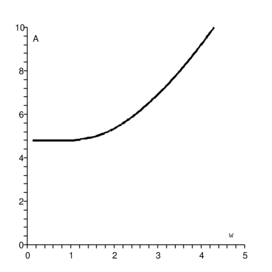
Figure 6. Graph of the function $A(\omega)$ defined by (192), in the case $\beta=-0.5$, obtained numerically.

Conjecture 48.

If $\beta<0$ then

(199) $$\lim_{\omega\rightarrow 0}A^{\prime}(\omega)=0.$$

Conjecture 49.

If $\beta<0$ then $A(\omega)$ is a convex function.

Lemma 50.

Let

(200) $$g(\omega)=\frac{A(\omega)}{\Upsilon(\omega)},\;\;\;\omega>0$$

where A is continuous function satisfying (196), (197), (199), and $\Upsilon$ is continuous, increasing and concave and satisfies (193),(194),(195). Then the function $g$ has a global minimum at $\omega_{0}>0$, and satisfies

(201) $$\lim_{\omega\rightarrow\infty}{g(\omega)}=+\infty.$$

If, moreover, $A$ is convex, then $g$ is decreasing on $[0,\omega_{0})$ and increasing on $(\omega_{0},\infty)$.

proof: We note first that (201) follows from (196),(195). We have

$$g^{\prime}(\omega)=\frac{A^{\prime}(\omega)\Upsilon(\omega)-A(\omega)\Upsilon^{\prime}(\omega)}{(\Upsilon(\omega))^{2}},$$

so (197),(199) and (194) imply that

(202) $$g^{\prime}(0)<0,$$

so $g$ is decreasing near $\omega=0$. Therefore the global minimum of $g$ is attained at some $\omega_{0}>0$.

Assuming now that $A$ is convex, we have

$$g^{\prime\prime}(\omega)=\frac{A^{\prime\prime}(\omega)\Upsilon(\omega)-A(\omega)\Upsilon^{\prime\prime}(\omega)}{(\Upsilon(\omega))^{2}}+\frac{2\Upsilon^{\prime}(\omega)[A^{\prime}(\omega)\Upsilon(\omega)-A(\omega)\Upsilon^{\prime}(\omega)]}{(\Upsilon(\omega))^{3}}.$$

The first term above is always positive because $A$ is convex and $\Upsilon$ is concave. This implies the following key property of $g$:

(203) $$g^{\prime}(\omega)\geq 0\;\;\Rightarrow\;\;g^{\prime\prime}(\omega)>0.$$

We note that by (201) there must exist some $\omega>0$ with $g^{\prime}(\omega)>0$. Let us define

$$\omega_{0}=\inf\{\omega>0\;|\;g^{\prime}(\omega)\geq 0\}.$$

By (202), we have $\omega_{0}>0$. From (203) it easily follows that that if $\omega>\omega_{0}$ then $g^{\prime}(\omega)>0$. By definition of $\omega_{0}$ we have $g^{\prime}(\omega)<0$ for all $\omega\in[0,\omega_{0})$. The lemma is thus established.

We thus have the following results

Lemma 51.

Assume $J$ satisfies (22), (23) and (174). Assume that conjecture 48 above is valid. Then when $\beta<0$, $g_{0}(\omega)$ has a global minimum at some $\omega_{0}>0$.

Lemma 52.

Assume $J$ satisfies (22), (23) and (174). Assume that both conjectures 48 and 49 above are valid. Then when $\beta<0$, $g_{0}(\omega)$ has a global minimum at some $\omega_{0}>0$, and is decreasing on $(0,\omega_{0})$ and increasing on $(\omega_{0},\infty)$.

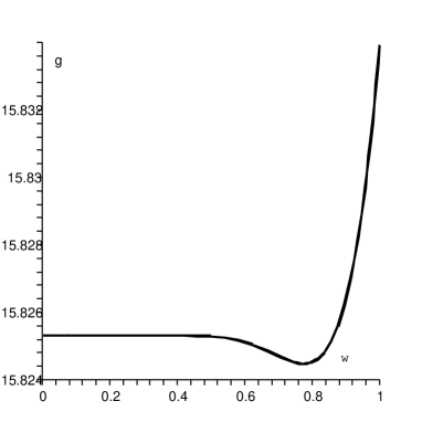
Figure 7. Graph of the function $g_{0}(\omega)$ in the case $J(z)=e^{-|z|}$, $\beta=-0.5$, $c=1$, obtained numerically.

In figure 7 we plot the function $g_{0}(\omega)$, when $\beta=-0.5$ and $c=1$, obtained by solving the equation $\Psi_{0}(\omega,g_{0}(\omega))=1$ for $g_{0}(\omega)$ numerically, where $\Psi_{0}$ is defined by (179). The qualitative properties claimed in lemma 52 can be seen in this plot.

Thus, in the case $\beta<0$, when $g$ is sufficiently large the frequencies of the fast and the slow travelling waves approach two positive values as $k\rightarrow 0$ (part (II)(ii) of the lemma), while if

(204) $$g_{crit}(0)<g_{0}(0)$$

part (II)(iii) of theorem 44 implies that we have a range of values of $g$ for which the frequency of the slow wave approaches $0$ as $k\rightarrow 0$. We note that, by definition, $g_{crit(0)}\leq g_{0}(0)$, so to show that case (ii) corresponds to a non-empty interval of values of $g$ we need only to show that the last inequality is strict. This follows at once from the conclusion of lemma 51, so that it is true modulo the validity of conjecture 48.

Furthermore if we assume that both conjectures 48 and 49 are valid, then lemma 52 tells us that $g_{0}(\omega)$ is unimodal, so we obtain the following strengthening of theorem 44:

Theorem 53.

Assume $J$ satisfies (22), (23) and (174). Suppose that conjectures 48 and 49 are valid. Assume $\beta<0$, and let $g_{crit}(0)=\min_{\omega>0}{g_{0}(\omega)}$. Then $g_{0}(0)>g_{crit}(0)$, and

(i) If $g<g_{crit}(0)$ then for sufficiently small $k>0$ there are no periodic travelling waves with wave-number $k$.

(ii) If $g_{crit}(0)<g<g_{0}(0)$, then (187) has precisely two solutions $0<\underline{\omega}<\overline{\omega}<\infty$, and for sufficiently small $k>0$ there are at least two periodic travelling waves with wave-number $k$ with the frequencies of the slow and fast waves approaching $\underline{\omega}$ and $\overline{\omega}$ as $k\rightarrow 0$.

(iii) If $g>g_{0}(0)$ then (187) has a unique solution $\omega$, and for sufficiently small $k>0$ there are at least two periodic travelling waves with wave-number $k$, and the frequency of the slow and fast waves approaches $0$ and $\omega$, respectively, as $k\rightarrow 0$.

We now present the results of some numerical computations of the functions $g_{k}(\omega)$ for small values of $k$. In these we encounter phenomenon not predicted by theorem 53 (though of course it does not contradict it). We fix $J(x)=e^{-|z|}$, $\beta=-1$ and $c=1$. In figure 8 we plot the numerically-computed functions $g_{k}(\omega)$ for several small values of $k$, as well as the function $g_{0}(\omega)$. We see that as $k\rightarrow 0$. $g_{k}(\omega)$ converges to $g_{0}(\omega)$ uniformly on compact subsets of $(0,\infty)$. However we now see that for sufficiently small $k$ the function $g_{k}$ has not one but two minima. One of these minima approaches the minimum of $g_{0}(\omega)$ as $k\rightarrow 0$, while the other one approaches $0$. The observed shape of $g_{k}(\omega)$ shows that for some values of $k$ and $g$ there exist four periodic waves of wave-number $k$! It would be interesting to gain a better understanding of the phenomena just described, both by means of more systematic numerical investigations and if possible also by analytical means.

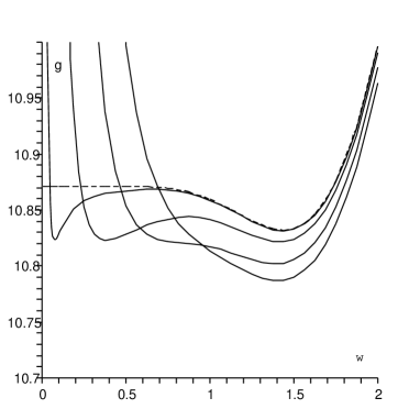
Figure 8. Numerically computed graphs of the functions $g_{k}(\omega)$ in the case $J(z)=e^{-|z|}$, $\beta=-1$, $c=1$, for the values $k=0.15$, $k=0.1$, $k=0.05$, $k=0.01$, and, in dashed line, $k=0$.

10. The question of stability

A crucial set of questions which are not addressed in our investigations, and remain open for now, is the relevance of the rotating waves on a ring, and of the periodic travelling waves on a line, in terms of the full dynamical problem given by (2), (3). The general question, as with all dynamical systems, is how arbitrary initial conditions develop in the long-time limit. More particularly, we would like to know whether the rotating waves on a ring and periodic travelling waves on a line describe this asymptotic behavior, at least in some cases.

A first step would be to determine the stability of the waves whose existence was proved here as solutions of the full dynamical problem. Let us note that the case of rotating wave on a ring and of a periodic travelling wave on a line should be distinguished here: if we can show that a rotating wave on a ring is asymptotically stable, then it does not imply that the corresponding periodic travelling wave on a line is stable - but rather only that it is stable to perturbations which have the same wave-number. Indeed, since in the case of a line, since we have a continuum of possible periodic travelling waves for different wave-numbers $k$, the best that we can expect is some kind of ‘neutral stability’ of the periodic travelling waves. If indeed there is convergence (in some sense) to a periodic travelling waves from general initial condition, the interesting question arises as to how the wave number of limiting wave is selected.

Based on analytical numerical results on other models [1, 7, 8, 9], we may conjecture that, at least under some natural assumptions on the synaptic coupling kernels $K(x)$ (in the case of a ring), $J(x)$ (in the case of a line), the fast wave is stable and the slow one is unstable. At our current state of knowledge analytical results may be hard to obtain (but see [10] for some analytical progress on related stability questions), so at least a systematic numerical investigation of the full dynamics of (2), (3) would be of much interest.

References

[1] P.C. Bressloff, Travelling waves and pulses
in a one-dimensional network of excitable integrate-and-fire
neurons, J. Math. Biol. 40 (2000), 169-198.
[2] G.B. Ermentrout, Type I membranes, phase
resetting curves and synchrony, Neural Comput. 8 (1996),
979-1001.
[3] G.B. Ermentrout & N. Kopell, Parabolic bursting in
an excitable system coupled with a slow oscillation, SIAM J.
Appl. Math. 46 (1986), 233-253.
[4] G.B. Ermentrout & J. Rinzel, Waves in a simple,
excitable or oscillatory, reaction-diffusion model, J. Math.
Biology 11 (1981), 269-294.
[6] E.M. Izhikevich, Class 1 neural excitability,
conventional synapses, weakly connected networks, and mathematical
foundations of pulse-coupled models, IEEE Trans. Neural Networks
10 (1999), 499-507.
[7] R. Osan & B. Ermentrout, Two dimensional synaptically generated travelling
waves in a theta-neuron neuronal network, Neurocomputing
38-40 (2001), 789-795.
[8] R. Osan, J. Rubin & B. Ermentrout, Regular
travelling waves in a network of Theta neurons, SIAM J. Appl.
Math. 62 (2002), 1197-1221.
[9] R. Osan, R. Curtu, J. Rubin, & B. Ermentrout,
Multiple-spike waves in a one-dimensional integrate-and-fire
neural network, J. Math. Biol. 48 (2004), 243-274.
[10] J.E. Rubin, A nonlocal eigenvalue problem for
the stability of a travelling wave in a neuronal medium,
Discrete & Continuous Dynamical Systems 10, (2004),
925-940.