Enhanced tracer transport by the spiral defect chaos state of a convecting fluid

Abstract

To understand how spatiotemporal chaos may modify material transport, we use direct numerical simulations of the three-dimensional Boussinesq equations and of an advection-diffusion equation to study the transport of a passive tracer by the spiral defect chaos state of a convecting fluid. The simulations show that the transport is diffusive and is enhanced by the spatiotemporal chaos. The enhancement in tracer diffusivity follows two regimes. For large Péclet numbers (that is, small molecular diffusivities of the tracer), we find that the enhancement is proportional to the Péclet number. For small Péclet numbers, the enhancement is proportional to the square root of the Péclet number. We explain the presence of these two regimes in terms of how the local transport depends on the local wave numbers of the convection rolls. For large Péclet numbers, we further find that defects cause the tracer diffusivity to be enhanced locally in the direction orthogonal to the local wave vector but suppressed in the direction of the local wave vector.

I Introduction

This paper addresses the transport of passive neutrally buoyant tracers in Rayleigh-Bénard convection exhibiting spiral defect chaos — an example of spatiotemporal chaos that is characterized by disorder in both space and time Cross and Hohenberg (1994); Gollub and Cross (2000); Hohenberg and Shraiman (1989). An important characteristic of such spatially disordered flows is that fluctuations in space play a significant role in their dynamics, resulting in advection of the passive tracers that is dependent in a complex fashion on space and time. The transport of passive tracers in such disordered flows is then governed by this advection in addition to molecular diffusion. The goal of this paper is to understand the net average transport of passive tracers as a function of the two competing mechanisms of advection by spatiotemporal chaos and molecular diffusion. Understanding material transport by spatiotemporal chaos is a problem that is of considerable importance in many branches of science and engineering. For example, an improved understanding may allow one to gain insight into heat and mass transport in atmospheric and oceanic flows and also in chemical engineering processes such as combustion.

Previous studies of the properties of passive transport in convective flows have focused only on the steady and weakly oscillatory regimes. For example, in two-dimensional time-independent laminar Rayleigh-Bénard convection flow, experiments have shown that the transport is effectively diffusive in the long time limit, with an effective diffusivity that is greater than the molecular diffusivity by a factor that scales as the square root of the Péclet number (defined in Eq. (14) to be the ratio of the strength of advection to diffusion) Solomon and Gollub (1988a). This enhancement, in the large Péclet number limit, has also been calculated theoretically by using the matched asymptotic expansion method Rosenbluth et al. (1987); Shraiman (1987). In addition, higher-order corrections to the diffusion process, for arbitrary Péclet numbers, have been calculated numerically using the homogenization method McCarty and Horsthemke (1988); McLaughlin et al. (1985). For nearly two-dimensional time-periodic convection, experiments near the onset of the oscillatory instability Busse (1978) have shown that the transport is again effectively diffusive but with an effective diffusivity that depends linearly on the local amplitude of the roll oscillations Solomon and Gollub (1988b). This result has also been confirmed in theoretical work, which also identified the invariant structures of the flow that acted as templates for the motion of the tracers Camassa and Wiggins (1991a, b). Passive tracer transport has also been studied in other types of laminar flow, including capillary waves generated by the Faraday instability Ramshankar et al. (1990); Ramshankar and Gollub (1991) and Taylor-Couette flow in a rotating annulus Solomon et al. (1993, 1994).

In this paper, the above transport studies are extended to flows that exhibit spatiotemporal chaos. It will be shown that the transport is globally diffusive and is enhanced by the spatiotemporal chaos. However, unlike the case of laminar flows, the enhancement is found to follow two regimes. For large Péclet numbers (that is, small molecular diffusivities of the tracer), the enhancement is proportional to the Péclet number, whereas for small Péclet numbers, the enhancement is proportional to the square root of the Péclet number. These two regimes are then explained by analyzing how the local transport depends on the local wave numbers of the convection rolls.

The remainder of this paper is organized as follows. In Sect. II, the equations governing Rayleigh-Bénard convection and the transport of passive tracers are defined. In addition, direct numerical simulations of these equations are discussed. In Sect. III, results from these simulations are presented. In Sect. IV, conclusions are presented.

II Equations and Algorithms

II.1 Rayleigh-Bénard Convection

In a typical Rayleigh-Bénard convection experiment, an incompressible fluid layer is confined between two horizontal plates, and is thermally driven far from equilibrium by maintaining the bottom plate at a temperature that is higher than that of the top plate. As the temperature difference is increased, the fluid undergoes an instability to a state in which there is motion driven by the buoyancy forces. When the temperature difference between the plates is above but near this convective threshold, a pattern comprising patches of locally parallel convection rolls forms with roll diameters that are close to the depth of the cell. When the temperature difference is increased, the fluid undergoes other instabilities that may result in the pattern developing an oscillatory or chaotic time-dependence. Finally when the temperature difference is increased further and if the aspect ratio $\Gamma$ is larger than about $20$ in boxes and $30$ in cylinders, spiral defect chaos appears. This state is a disordered collection of spirals that rotate in both directions and coexist with dynamical defects such as grain boundaries and dislocations. Fig. 1 shows a numerically simulated instance of the spiral defect chaos state in a cylindrical geometry. More generally, spiral defect chaos is an example of a kind of widely observed phenomenon called spatiotemporal chaos that exhibits disorder in space and chaos in time.

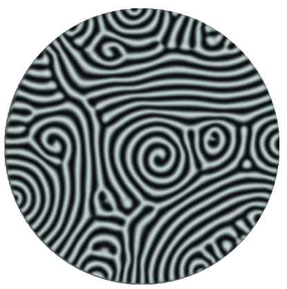
Figure 1: Example of spiral defect chaos observed in a numerical simulation described in Sect. II.3 with insulating and no-slip boundaries, and with a spatial resolution of $\Delta x=1/8$ and a temporal resolution of $\Delta t=10^{-3}$. The mid-plane temperature field is plotted at time $t=500$ for parameters $\epsilon=1.0$, $\sigma=1$, and in a cylindrical geometry of aspect ratio $\Gamma=30$. Dark regions correspond to cold sinking fluid, light regions to hot rising fluid. The spiral defect chaos planform is characterized by a disordered collection of spirals rotating in both directions and coexisting with dynamical defects such as grain boundaries and dislocations.

The evolution of the convecting fluid is governed to good approximation by the three-dimensional Boussinesq equations Cross and Hohenberg (1993). They are the combination of the incompressible Navier-Stokes and heat equations, with the further assumption that density variations are proportional to temperature variations and that this density variation appears only in the buoyancy force. Written in a dimensionless form, they are:

$$\sigma^{-1}\left(\partial_{t}+\mathbf{u}\,{\scriptscriptstyle\stackrel{{\scriptstyle\bullet}}{{{}}}}\,\mathbf{\nabla}\right)\mathbf{u}(x,y,z,t) = -\mathbf{\nabla}p+\mathbf{\nabla}^{2}\mathbf{u}+RT\widehat{z},$$ (1)

$$\left(\partial_{t}+\mathbf{u}\,{\scriptscriptstyle\stackrel{{\scriptstyle\bullet}}{{{}}}}\,\mathbf{\nabla}\right)T(x,y,z,t) = \mathbf{\nabla}^{2}T,$$ (2)

$$\mathbf{\nabla}\,{\scriptscriptstyle\stackrel{{\scriptstyle\bullet}}{{{}}}}\,\mathbf{u} = 0.$$ (3)

The field $\mathbf{u}(x,y,z,t)$ is the velocity field at point $(x,y,z)$ at time $t$, while $p$ and $T$ are the pressure and temperature fields, respectively. The variables $x$ and $y$ denote the horizontal coordinates, while the variable $z$ denotes the vertical coordinate, with the unit vector $\widehat{z}$ pointing in the direction opposite to the gravitational acceleration. The spatial units are measured in units of the cell depth $d$, and time is measured in units of the vertical thermal diffusion time $d^{2}/\kappa$, where $\kappa$ is the thermal diffusivity of the fluid. The parameter $R$ is the Rayleigh number, a dimensionless measure of the temperature difference $\Delta T$ across the top and bottom plates,

$$R=\frac{\alpha gd^{3}}{\nu\kappa}\Delta T,$$ (4)

where $\alpha$ is the thermal expansion coefficient, $\kappa$ the thermal diffusivity, and $\nu$ the viscous diffusivity (kinematic viscosity) of the fluid. In this paper, the reduced Rayleigh number will also be frequently used,

$$\epsilon=\frac{R-R_{c}}{R_{c}},$$ (5)

where $R_{c}\approx 1708$ is the critical Rayleigh number at the onset of convection in an infinite domain Cross and Hohenberg (1993). The parameter $\sigma$ is the Prandtl number, defined to be the ratio of the fluid’s thermal to viscous diffusivities,

$$\sigma=\frac{\nu}{\kappa}.$$ (6)

The material walls are no-slip so that the velocity field satisfies

$$\mathbf{u}=\mathbf{0},\ \ \ \mbox{on all material walls}.$$ (7)

The temperature field is constant on the top and bottom plates:

$$T\left(x,y,z=\mp\frac{1}{2},t\right)=\pm\frac{1}{2}.$$ (8)

The lateral walls are assumed to be perfectly insulating, so that

$$\widehat{n}\,{\scriptscriptstyle\stackrel{{\scriptstyle\bullet}}{{{}}}}\,\mathbf{\nabla}T=0,\ \ \ \mbox{on lateral walls,}$$ (9)

where $\widehat{n}$ is the unit vector perpendicular to the lateral walls at a given point. The pressure field $p$ has no associated boundary condition because it does not satisfy a dynamical equation.

The influence of the lateral walls on the dynamics is determined by the dimensionless aspect ratio $\Gamma$, defined to be the half-width-to-depth ratio of the cell if it is rectangular and the radius-to-depth ratio if it is cylindrical.

II.2 Transport Equation

The transport of passive neutrally buoyant tracers in a flow can be described by the advection-diffusion equation. Written in a dimensionless form, it is

$$(\partial_{t}+\mathbf{u}\,{\scriptscriptstyle\stackrel{{\scriptstyle\bullet}}{{{}}}}\,\mathbf{\nabla})\psi(x,y,z,t)=\mathcal{L}\mathbf{\nabla}^{2}\psi.$$ (10)

The scalar field $\psi(x,y,z,t)$ is the passive tracer concentration at point $(x,y,z)$ and time $t$. The velocity field $\mathbf{u}$ is obtained by solving the Boussinesq equations, Eqs. (1)–(3). The parameter $\mathcal{L}$ is the Lewis number, defined to be the molecular diffusivity $D$ of the tracers made dimensionless by the thermal diffusivity $\kappa$ of the fluid,

$$\mathcal{L}=\frac{D}{\kappa}.$$ (11)

In this paper, small Lewis numbers in the range $10^{-3}\leq\mathcal{L}\leq 10^{-1}$ will be considered. In comparison, the Lewis numbers of passive tracers used in previous convection experiments Solomon and Gollub (1988a) in water at approximately $300$ K, namely, micrometer-sized latex spheres (vinyl toluene $t$-butylstyrene) and methylene blue dye, are $\mathcal{L}=1.2\times 10^{-5}$ and $\mathcal{L}=3.9\times 10^{-3}$, respectively.

The tracers are assumed to be passive, that is, their motions in the fluid do not modify the fluid’s velocity field. The fluid is also assumed to have negligible Soret and Dufour effects. The former refers to the additional passive tracer concentration current driven by gradients of the temperature field, whereas the latter refers to the additional heat current driven by gradients of the passive tracer concentration. In addition, the lateral walls are assumed to be impermeable to the tracers, so that

$$\widehat{n}\,{\scriptscriptstyle\stackrel{{\scriptstyle\bullet}}{{{}}}}\,\mathbf{\nabla}\psi=0\ \ \ \mbox{on lateral walls,}$$ (12)

where $\widehat{n}$ is the unit vector perpendicular to the lateral walls at a given point.

Eq. (10) is also commonly written in the literature in an alternate but entirely equivalent form. By dividing it throughout by the product of a characteristic velocity scale $||\mathbf{u}||$ and a characteristic length scale, Eq. (10) becomes

$$(\partial_{\tilde{t}}+\mathbf{\tilde{u}}\,{\scriptscriptstyle\stackrel{{\scriptstyle\bullet}}{{{}}}}\,\mathbf{\nabla})\psi(x,y,z,t)=\frac{1}{\mathcal{P}}\mathbf{\nabla}^{2}\psi,$$ (13)

with $\tilde{t}$ the rescaled time, $\mathbf{\tilde{u}}$ the rescaled velocity field, and $\mathcal{P}$ the Péclet number, defined to be the dimensionless ratio of the relative importance of the advection of the tracers to their molecular diffusion,

$$\mathcal{P}=\frac{||\mathbf{u}||}{\mathcal{L}}.$$ (14)

(Note that the numerator in Eq. (14) contains a characteristic length scale — the depth of the cell — which is unity and is thus omitted.)

Finally, it should also be noted that instead of studying the passive tracer concentration field $\psi$ in the space coordinates defined in the laboratory frame (the Eulerian approach), one could study the trajectories of each passive tracer individually (the Lagrangian approach) by integrating, for each passive tracer,

$$\frac{d\mathbf{x}(t)}{dt}=\mathbf{u}[\mathbf{x}(t),t]+\mathbf{\eta}(t),$$ (15)

where $\mathbf{x}(t)$ is the position of the tracer [initially at $\mathbf{x}(0)$], $\mathbf{u}$ is the Eulerian velocity field at space $\mathbf{x}(t)$ and time $t$, and $\mathbf{\eta}(t)$ is a Langevin noise introduced to represent molecular diffusion. However, this approach is not pursued here because of the difficulties associated with integrating Eq. (15). In fact, even if the velocity field $\mathbf{u}$ can be explicitly determined and has a very simple form, the tracer trajectories $\mathbf{x}$ can have very complicated dynamics Aref (1983).

II.3 Direct Numerical Simulations

We use a parallel spectral element scheme to integrate the Boussinesq equations, Eqs. (1)–(3), and the transport equation, Eq. (10). The scheme is second-order-accurate in time and is designed for rectangular, cylindrical, as well as more complex geometries with arbitrary lateral boundary conditions. Details of this scheme are available elsewhere Fischer (1997). For applications of this scheme to related problems in Rayleigh-Bénard convection, see Refs. Paul et al. (2003); Chiam et al. (2003); Paul et al. (2001, 2002, 2004).

For small Lewis numbers $\mathcal{L}\ll 1$, one well-known difficulty Fletcher (1991); Tannehill et al. (1997) associated with integrating Eq. (10) is that the spatial resolution $\Delta x$ has to be very small. This scale is set by the smallest scale in the tracer concentration field, such as the thickness of the interface where the tracer is initially zero on one side and unity on the other. The interface is then stretched by a strain rate $S\sim\partial u/\partial x\sim||\mathbf{u}||$, and its thickness is proportional to $(\mathcal{L}/S)^{1/2}$, that is,

$$\Delta x\sim\left(\frac{\mathcal{L}}{||\mathbf{u}||}\right)^{1/2}=\mathcal{P}^{-1/2}.$$ (16)

For the spiral defect chaos states considered in this paper, the velocity magnitude, $||\mathbf{u}||$, is about $10$. Thus, a simulation at the Lewis number of, say, $\mathcal{L}=10^{-3}$ will require $\Delta x\sim 10^{-2}$ in order to satisfy Eq. (16). However, current computational resources dictate that $\Delta x$ be about $\,{\scriptscriptstyle\stackrel{{\scriptstyle>}}{{\sim}}}\,10^{-1}$, and in fact, for the results quoted in this paper, $\Delta x=1/8$. This problem is overcome by using a filtering procedure developed by Fischer and Mullen Fischer and Mullen (2001), and is described in Appendix A. Using this filter and maintaining $\Delta x=1/8$, a Lewis number as small as $\mathcal{L}=10^{-3}$ can be attained in a stable simulation. The accuracy of using the filter is also discussed in the Appendex.

III Results

The transport equation, Eq. (10), was integrated concurrently with the Boussinesq equations, Eqs. (1)–(3), for the following parameters: the Rayleigh number varied from the onset of spiral defect chaos at $R\approx 3000$ to fully developed spiral defect chaos at $R\approx 4000$, the Prandtl number $\sigma=1$, and the Lewis number ranging from $\mathcal{L}=10^{-3}$ to $\mathcal{L}=10^{-1}$. The direct numerical simulations have been performed in cylindrical three-dimensional cells of various aspect ratios. In this paper, data for an aspect ratio of $\Gamma=30$ will be reported. The initial condition used for the passive tracer concentration field is a localized concentration at the center of the cell:

$$\psi(x,y,z,t=0)=\exp\left[-\frac{x^{2}+y^{2}+z^{2}}{6\Delta^{2}}\right],$$ (17)

with $\Delta=1/4$ a small constant to ensure that the passive tracer concentration is initially localized. At time $t=0$, the temperature, velocity, and pressure fields correspond to an asymptotic state of spiral defect chaos, that is, one that has been evolved from random thermal perturbations up to a time of $\mathcal{O}(\Gamma^{2})$. In this paper, the focus will be on cells of large aspect ratio, $\Gamma\geq 20$. For these aspect ratios, the $z$-dependence of the passive tracer concentration field was found to be essentially constant. As such, the $z$-dependence will be dropped in subsequent discussions and the passive tracer concentration $\psi(x,y,t)$ will be considered as a function of two-dimensional horizontal space and time.

In Fig. 2, the evolution of the passive tracer concentration field $\psi(x,y,t)$ at the mid-plane $z=0$ for the parameters $R=3500$, $\sigma=1$, and $\mathcal{L}=10^{-2}$ is shown for various times $t$. The passive tracer concentration spreads outward with time in a non-uniform and non-axisymmetric way. In Sect. III.1, this spreading is quantified globally by studying the mean square displacement of the passive tracer concentration field. In Sect. III.2, this spreading is shown to be characterized by normal diffusion. In Sect. III.3, the local dependence of the spreading on the local wave number is discussed.

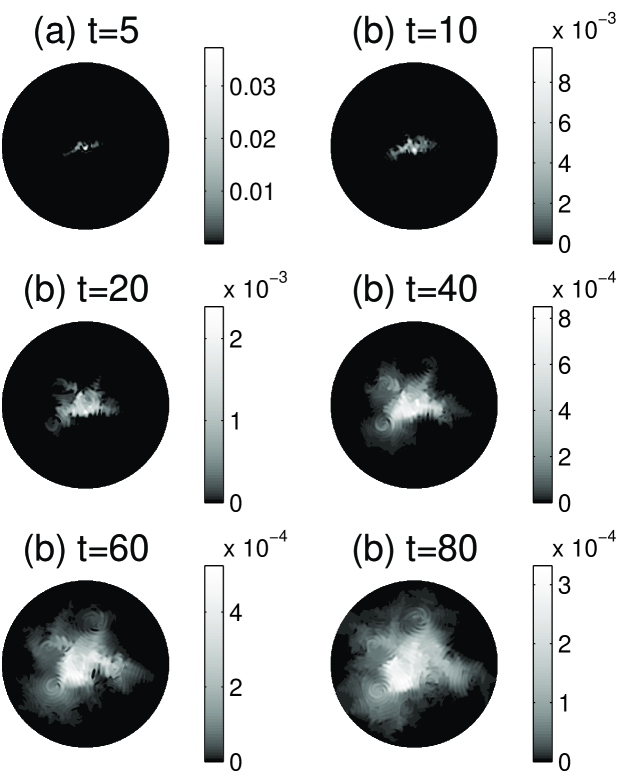
Figure 2: Evolution of the passive tracer concentration field $\psi(x,y,z=0,t)$ for various times $t$, obtained by numerically solving Eq. (10). The Rayleigh number $R=3500$, the Prandtl number $\sigma=1$, and the Lewis number $\mathcal{L}=10^{-2}$, and the cylindrical cell has the aspect ratio $\Gamma=30$. The initial condition for $\psi$ at $t=0$ is given by Eq. (17).

III.1 Statistics of moments of passive tracer concentration

The spreading of the passive tracers can be quantified by its mean square displacement $M_{2}(t)$, or the second moment, of the passive tracer concentration field,

$$M_{2}(t)=\frac{\int_{0}^{\Gamma}\int_{0}^{2\pi}|\mathbf{x}-\langle\mathbf{x}\rangle(t)|^{2}\psi(r,\theta,t)\,r\,dr\,d\theta}{\int_{0}^{\Gamma}\int_{0}^{2\pi}\psi(r,\theta,t)\,r\,dr\,d\theta}.$$ (18)

Here, $\mathbf{x}=(r,\theta)$ is the polar coordinate with origin at the center of the cell. In practice, $M_{2}(t)$ is computed as the average over different instances (typically three to five) of $\psi$ obtained from different random initial conditions of spiral defect chaos, that is, the velocity, temperature, and pressure fields used at $t=0$ are different instances of fully developed spiral defect chaos. The quantity $\langle\mathbf{x}\rangle(t)$ is the instantaneous center of mass of the tracer distribution,

$$\langle\mathbf{x}\rangle(t)=\frac{\int_{0}^{\Gamma}\int_{0}^{2\pi}\mathbf{x}\psi(r,\theta,t)\,r\,dr\,d\theta}{\int_{0}^{\Gamma}\int_{0}^{2\pi}\psi(r,\theta,t)\,r\,dr\,d\theta}.$$ (19)

In Fig. 3, the mean square displacement $M_{2}(t)$ is plotted for several different values of the Rayleigh number $R$ and the Lewis numbers $\mathcal{L}=10^{-3}$ and $\mathcal{L}=10^{-2}$. It is found that, in all cases, the mean square displacement $M_{2}(t)$ is directly proportional to the time $t$ to a very good approximation. Least squares fits of $M_{2}(t)$ to power laws $\sim t^{\gamma}$ yield exponents $\gamma$ of approximately unity, as shown in Table 1.

	$\mathcal{L}$	$10^{-2}$	$10^{-3}$
$R$
$3074$		1.1	1.1
$3500$		1.0	1.1
$4270$		1.1	1.1

Table 1: The exponent $\gamma$ computed from the fit of the mean square displacement $M_{2}(t)$ to a power law $\sim t^{\gamma}$ for several different values of the Rayleigh number $R$ and Lewis number $\mathcal{L}$. It is approximately unity in all instances.

This implies that the spreading of the passive tracer concentration field can be described by a normal diffusive process. In other words, the averaged passive tracer concentration, $\bar{\psi}(r,t)$, evolves according to the one-dimensional normal diffusion equation,

$$\partial_{t}\tilde{\psi}(r,t)=\mathcal{L}^{\ast}\partial_{rr}\tilde{\psi}$$ (20)

with $\mathcal{L}^{\ast}$ an effective Lewis number that can be extracted from the mean square displacement as

$$M_{2}(t)=4\mathcal{L}^{\ast}t.$$ (21)

Several values of the effective Lewis number for various values of the parameters are tabulated in Table 2.

	$\mathcal{L}$	$10^{-3}$	$10^{-2}$	$10^{-1}$
$R$
$3074$		0.29	0.29	0.38
$3500$		0.35	0.35	0.50
$4270$		0.42	0.41	0.53

Table 2: The effective Lewis number $\mathcal{L}^{\ast}$ computed from Eq. (21) for various values of the Rayleigh number $R$ and the Lewis number $\mathcal{L}$.

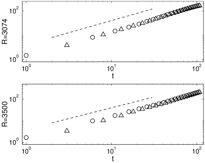
Figure 3: The mean square displacement $M_{2}(t)$ of the passive tracer concentration field for two different Rayleigh numbers $R=3074$ (top) and $3500$ (bottom). The Prandtl number is $\sigma=1$ in both cases. The triangle and circle symbols denote data for the Lewis number $\mathcal{L}=10^{-3}$ and $\mathcal{L}=10^{-2}$, respectively. The dashed lines have slopes of unity. The exponents obtained from power law fits of the data are given in Table 1.

The quantity

$$\Delta\equiv\frac{\mathcal{L}^{\ast}-\mathcal{L}}{\mathcal{L}}$$ (22)

is then a dimensionless measure of the enhancement in the molecular diffusivity of the passive tracer concentration brought upon by the advection of the spiral defect chaotic flow. The goal of this paper can then be phrased as the calculation of how this enhancement varies as a function of both the properties of the advecting fluid (the Rayleigh number $R$ and Prandtl number $\sigma$) and the property of the passive tracer concentration [its Lewis number, or equivalently, the Péclet number, $\mathcal{P}$, c.f. Eq. (14)],

$$\Delta=\Delta(R,\sigma,\mathcal{P}).$$ (23)

The results of this calculation are shown in Fig. 4, which depicts how the enhancement $\Delta$ varies vs. the Péclet number $\mathcal{P}$ for various Rayleigh numbers $R$ and the Prandtl number $\sigma=1$.

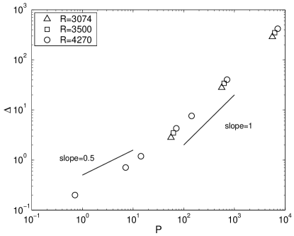
Figure 4: The dimensionless enhancement in molecular diffusivity $\Delta$ defined in Eq. (22) vs. the Péclet number $\mathcal{P}$ for various Rayleigh numbers $R$ and the Prandtl number $\sigma=1$. Note that, when the Péclet number approaches zero (that is, when the advection becomes negligible so that the transport equation, Eq. (10), is the diffusion equation), the enhancement should approach zero as well. Thus, the data points are expected to pass through the origin $(\mathcal{P}=0,\Delta=0)$.

It is found that the enhancement $\Delta$ follows two different scaling regimes in the Péclet number $\mathcal{P}$. In the regime of large Péclet numbers, $\mathcal{P}\,{\scriptscriptstyle\stackrel{{\scriptstyle>}}{{\sim}}}\,10^{2}$, the enhancement is found to scale linearly with the Péclet number,

$$\Delta\propto\mathcal{P}.$$ (24)

This implies that the effective Lewis number also scales linearly with the velocity magnitude of the flow, and is independent of the Lewis number $\mathcal{L}$,

$$\mathcal{L}^{\ast}-\mathcal{L}\propto||\mathbf{u}||.$$ (25)

[Eq. (25) is easily obtained by dividing Eq. (24) by the Lewis number $\mathcal{L}$.] In addition, it is of interest to see how the effective Lewis number relates to the reduced Rayleigh number. This relation is plotted in Fig. 5, and it exhibits a square-root dependence,

$$\mathcal{L}^{\ast}-\mathcal{L}\propto\epsilon^{1/2}.$$ (26)

Thus, Eqs. (25) and (26) together suggest that the characteristic velocity scale of spiral defect chaos scales with the reduced Rayleigh number as

$$||\mathbf{u}||\propto\epsilon^{1/2}.$$ (27)

Figure 5: The effective Lewis number $\mathcal{L}^{\ast}-\mathcal{L}$ vs. the reduced Rayleigh number $\epsilon$. The solid line represents a power law with an exponent of $1/2$.

On the other hand, in the regime of small Péclet numbers, $\mathcal{P}\,{\scriptscriptstyle\stackrel{{\scriptstyle<}}{{\sim}}}\,10^{2}$, the enahancement is found to scale with the Péclet number as

$$\Delta\propto\mathcal{P}^{1/2}.$$ (28)

(Note that there are insufficient data to conclude whether the crossover between the two regimes is a continuous and gradual one or a discontinuous and sharp one.) This square root dependence of the enhancement on the Péclet number is similar to the result obtained experimentally Solomon and Gollub (1988a) and calculated theoretically Rosenbluth et al. (1987); Shraiman (1987) in the spreading of passive tracers in time-independent convection flows comprising straight parallel rolls. In this case, the enhancement can be attributed to the expulsion of the gradient of the passive tracer concentration from regions of closed stream lines Shraiman (1987). Near a separatrix between two sets of closed stream lines, the only transport of the passive tracers from one roll to the next comes from the random walks of the passive tracers that lie within a thin layer of width $d$ of the roll boundary (the roll itself is of unit width in the dimensionless unit system adopted in this paper). Thus, a fraction $d$ of passive tracers contribute to an increase, $d\mathcal{L}$, in the effective Lewis number of the diffusion. The width $d$ can be estimated from dimensional analysis Bohr et al. (1998) to be $d^{2}\sim\mathcal{P}^{-1}$. Combining these estimates leads immediately to Eq. (28). Thus, the result above suggests that the gradient expulsion mechanism near closed streamlines, although strictly derived in a time-independent convection flows comprising straight parallel rolls, may be a universal mechanism at sufficiently small Péclet numbers independent of the structure of the underlying flow field.

In Sect. III.3, the origin of these two distinct regimes is discussed in terms of the dependence on the local wave number of the convection rolls. But before concluding this section, some details are presented in the way the least squares fits were performed. First, data from early times are ignored because of the presence of transients. One such transient effect could be that, at very early times prior to the turnover time scale $\tau_{c}\sim||\mathbf{u}||^{-1}\sim\mathcal{O}(10^{-1})$, the passive tracers “feel” that they are being transported by a constant velocity field, and so will exhibit ballistic behavior with $\gamma=2$. There is then a crossover time in which $\gamma$ decreases to unity, and this regime is to be ignored too. Second, data from late times are also ignored because of finite size effects. The time at which finite size effects become important is chosen as the time at which the exponent $\gamma$, obtained from the logarithmic derivative

$$\gamma(t)=\frac{d\log[M_{2}(t)]}{d\log(t)},$$ (29)

deviates from approximately unity for a purely diffusive process with without advection (that is, whose diffusivity is chosen to match that of effective diffusivity of the above process).

III.2 Normal diffusion vs. anomalous diffusion

In this section, results are discussed from two other tests that show that the spreading process is indeed governed by normal diffusion, and not anomalous diffusion. Diffusion is said to be anomalous when the mean square displacement is not proportional to time, that is, when $M_{2}(t)\propto t^{\gamma}$ with the exponent $\gamma\neq 1$. Anomalous diffusion has been observed in the transport of passive tracers in cellular Taylor-Couette flow in a rotating annulus Solomon et al. (1993, 1994), and in various other geophysical turbulent flows arising from the presence of Lévy trajectories Shlesinger et al. (1995). However, results from this section show no evidence of anomalous diffusion in transport in spiral defect chaos for the range of Lewis numbers investigated.

First, if the passive tracer concentration is spreading by normal diffusion and so obeys Eq. (20), then it can be expressed in the form of a Gaussian,

$$\tilde{\psi}(r,t)\sim\frac{1}{t}\exp\left(\frac{r^{2}}{4\mathcal{L}^{\ast}t}\right),$$ (30)

and a plot of the logarithm of the scaled passive tracer concentration $\log[t\tilde{\psi}(r,t)]$ vs. the scaled distance $\sqrt{r^{2}/4t}$ for different times $t$ will all collapse onto the same curve. This is indeed the case, as shown in Fig. 6, which shows the data at times $t=30$, $t=40$, and $t=70$ (triangles, squares, and circles, respectively) collapsing onto the same straight line. However, data from an earlier time $t=5$ (crosses) do not collapse onto the same straight line, presumably because of the presence of transient effects. Similarly, data from a later time $t=100$ (dots) do not collapse onto the same straight line, because of the presence of finite size effects.

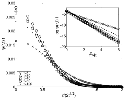
Figure 6: The scaled passive tracer concentration $t\tilde{\psi}(r,t)$ vs. the scaled distance $\sqrt{r^{2}/4t}$ and scaled distance squared $r^{2}/4t$ (inset). The various symbols denote different values of the times $t$. The data for times $t=30$, $t=40$, and $t=70$ (triangles, squares, and circles, respectively) collapse onto the same curve, suggesting the validity of the Gaussian form in this time range.

Second, possible deviations from the Gaussian behavior of the passive tracer concentration can be checked by looking at the higher-order moments,

$$M_{q}(t)=\frac{\int_{0}^{\Gamma}\int_{0}^{2\pi}|\mathbf{x}-\langle\mathbf{x}\rangle(t)|^{q}\psi(r,\theta,t)\,r\,dr\,d\theta}{\int_{0}^{\Gamma}\int_{0}^{2\pi}\psi(r,\theta,t)\,r\,dr\,d\theta}.$$ (31)

For normal diffusion, the higher-order moments scale like

$$M_{q}(t)\propto t^{q/2},$$ (32)

and the ratio of this higher-order moment scaled to the second-order moment can be calculated to be

$$\frac{M_{q}(t)^{2/q}}{M_{2}(t)}=1\cdot 3\cdots(q-1)=(q-1)!!$$ (33)

which is a constant in time. In Fig. 7, this scaled ratio is plotted for $q=4$, $6$, and $8$ as functions of time when the Rayleigh number $R=3500$, the Prandtl number $\sigma=1$, and the Lewis number $\mathcal{L}=10^{-2}$. The dashed lines show the corresponding quantity for a purely diffusive process with diffusivity chosen to match the former’s effective diffusivity. (Because of finite size effects, the scaled higher-order moments unfortunately have only a small range for which they are constant in time. For example, at $q=8$, this range is only $5\,{\scriptscriptstyle\stackrel{{\scriptstyle<}}{{\sim}}}\,t\,{\scriptscriptstyle\stackrel{{\scriptstyle<}}{{\sim}}}\,20$.) The agreement of the two sets of data shows that, apart from finite size effects, there are no discernible deviations from Gaussian form for the passive tracer concentrations.

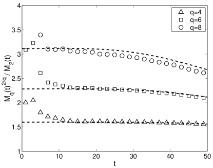
Figure 7: The ratio of the scaled higher-order moments to the second-order moment, $M_{q}(t)^{2/q}/M_{2}(t)$ , of the passive tracer concentration vs. time $t$ for the parameters $R=3500$, $\sigma=1$, and $\mathcal{L}=10^{-2}$, and for a purely diffusive process (dashed lines). From Eq. (33), this ratio is $1.73$ when $q=4$, $2.47$ when $q=6$, and $3.20$ when $q=8$. As $q$ increases, the range of time for which the scaled moment stays constant in time decreases, because of finite size effects.

Thus, both observations above suggest that the spreading of the passive tracer concentration is governed by normal diffusion.

III.3 Wave number dependence of the passive tracer transport

In this section, the existence of two different scaling regimes for the dimensionless enhancement in molecular diffusivity, namely at large Péclet numbers given by Eq. (24) and at small Péclet numbers given by Eq. (28), is investigated in terms of the local wave number dependence of the passive tracer concentration. To make this discussion more quantitative, first a quantity called the horizontal spreading orientation, $\Theta(x,y)$, is calculated at every location in the cell,

$$\cos(\Theta)=\frac{\mathbf{\nabla}_{\perp}\psi\,{\scriptscriptstyle\stackrel{{\scriptstyle\bullet}}{{{}}}}\,\mathbf{k}}{|\mathbf{\nabla}_{\perp}\psi||\mathbf{k}|}.$$ (34)

The subscript $\perp$ denotes the horizontal coordinates $(x,y)$ and $\mathbf{k}(x,y)$ is the local wave vector at location $(x,y)$ in the planform Egolf et al. (1998). If the passive tracer concentration spreads in the direction of the local wave vector $\mathbf{k}$, then, as illustrated in Fig. 8(a), the gradient $\mathbf{\nabla}_{\perp}\psi$ will be orthogonal to $\mathbf{k}$, resulting in the local horizontal spreading orientation acquiring the value of $\Theta=\pi/2$. On the other hand, if the passive tracer concentration spreads in the direction orthogonal to $\mathbf{k}$, then, as illustrated in Fig. 8(b), the local horizontal spreading orientation will be $\Theta=0$.

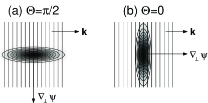
Figure 8: Illustrations showing the definition of the horizontal spreading orientation, $\Theta$, at (a) $\Theta=\pi/2$ corresponding to spreading in the direction of the local wave vector $\mathbf{k}$, and (b) $\Theta=0$ corresponding to spreading in the direction orthogonal to $\mathbf{k}$.

For a particular passive tracer concentration, the horizontal spreading orientation can be computed locally at every point in the mid-plane of the convection cell and then were sorted into bins to create a histogram. In Fig. 9, such a distribution of the horizontal spreading orientation, $P(\Theta)$, is plotted for several values of the Lewis number ranging from $\mathcal{L}=10^{-3}$ to $\mathcal{L}=10^{-1}$, the Rayleigh number $R=3500$, and the Prandtl number $\sigma=1$ at time $t=50$. Consider first the distribution for the relatively large Lewis number of $\mathcal{L}=10^{-1}$ (denoted by crosses). This distribution has a peak at $\Theta=\pi/2$. This suggests that the spreading of the passive tracer concentration has the highest probability to be in the direction of the wave vector $\mathbf{k}$ [that is, as illustrated in the scenario of Fig. 8(a)]. This is consistent with the gradient expulsion mechanism near closed streamlines described earlier in Sect. III.1. However, at the smaller Lewis numbers of, say, $\mathcal{L}=10^{-3}$, the distribution of the horizontal spreading orientation is visibly different. The distribution now has a peak at $\Theta=0$. In other words, the spreading of the passive tracer concentration has the highest probability in the direction orthogonal to the wave vector $\mathbf{k}$ [that is, as illustrated in scenario of Fig. 8(b)]. This shows that two different scaling regimes for the dimensionless enhancement in molecular diffusivity are associated with two different transport mechanisms. At large Lewis numbers (or equivalently, small Péclet numbers), the transport is along the direction of the wave vector $\mathbf{k}$ by the gradient expulsion mechanism. At small Lewis numbers (or equivalently, large Péclet numbers), the transport is orthogonal to the wave vector $\mathbf{k}$, presumably by advection by the disordered flow.

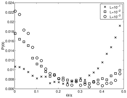
Figure 9: Distribution of horizontal spreading orientations $P(\Theta)$ for the Rayleigh number $R=3500$, the Prandtl number $\sigma=1$ and the Lewis number ranging from $\mathcal{L}=10^{-3}$ to $\mathcal{L}=10^{-1}$.

To determine why there is transport orthogonal to the wave vector $\mathbf{k}$ at small Lewis numbers (or equivalently, large Péclet numbers), the following calculation was performed. The local wave numbers that correspond to locations that exhibit spreading in the direction orthogonal to the wave vector $\mathbf{k}$ (that is, $0\leq\Theta\leq\eta$ where $\eta=0.01$ is a small constant) were compared with those locations that exhibit spreading in the direction of the wave vector $\mathbf{k}$ (that is, $\pi/2-\eta\leq\Theta\leq\pi/2$). In Fig. 10, the distribution of wave numbers $P(k,\Theta)$ for which the spreading occurs orthogonally to $\mathbf{k}$ (solid lines) is plotted together with the distribution for which spreading is along $\mathbf{k}$ (dashed lines) for a large Lewis number case [Fig. 10(a)] and a small Lewis number case [Fig. 10(b)]. The key point to observe is that, in the small Lewis number case, there is a higher probability that spreading occurs orthogonal to the wave vector ($\Theta\rightarrow 0$, solid line) than along the wave vector ($\Theta\rightarrow\pi/2$, dashed line) for wave numbers $k\approx 1.5$ and $k\approx 2.5$. These wave numbers, far away from the mean wave number, correspond to to the occurrence of defects such as spiral cores, target cores, dislocations, etc. This suggests that the reason why gradient expulsion ceases to be valid at large Péclet numbers is due to the enhanced transport of the passive tracers orthogonal to the local wave vectors by the defects in the pattern. However, the presence of defects is not sufficient to overcome the gradient expulsion mechanism at small Péclet numbers.

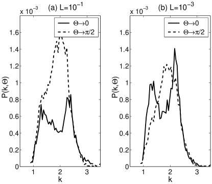
Figure 10: Distribution of wave numbers $P(k,\Theta)$ for which spreading occurs orthogonally to the local wave vector $\mathbf{k}$ (solid lines) and in the direction of $\mathbf{k}$ (dashed lines), for (a) large Lewis number $\mathcal{L}=10^{-1}$ and (b) small Lewis number $\mathcal{L}=10^{-3}$ at the Rayleigh number $R=3500$ and the Prandtl number $\sigma=1$.

IV Conclusions

In this paper, the spreading of a passive tracer concentration in a Rayleigh-Bénard convection flow exhibiting spiral defect chaos is studied for the first time. All previous studies have dealt with time-independent or oscillatory flows. In the presence of advection by spiral defect chaos, we find that the spreading continues to be characterized by normal diffusion. The enhancement follows two regimes. When the Péclet number is large (that is, when the molecular diffusivity of the tracer is small), the enhancement is proportional to the Péclet number. This means that in the limit of large Péclet number the effective diffusivity is independent of the molecular diffusivity, and is proportional to the strength of the advection velocity field. When the Péclet numbers is small, the enhancement is proportional to the square root of the Péclet number. These results are explained in terms of the dependence of the transport on the local wave numbers. It is found that tracers with small Péclet numbers follow the gradient expulsion mechanism described previously in time-independent flows Shraiman (1987) which predicts the square-root dependence. However, when the Péclet number becomes large, defects in the flow field became important and lead to enhanced transport orthogonal to the local wave vectors.

Appendix A Numerical details

As mentioned in Sect. II.3, for small Lewis numbers $\mathcal{L}\ll 1$, a difficulty associated with integrating the transport equation, Eq. (10), is that the spatial resolution $\Delta x$ must be small. A larger $\Delta x$ can be used by employing a simple filtering procedure developed by Fischer and Mullen Fischer and Mullen (2001). At the end of each time step, a filter is applied on an element-by-element basis to the passive tracer concentration field $\psi$. In one dimension, the filtered field can be written as

$$F(\psi;\alpha)=\alpha\Pi_{N-1}(\psi)+(1-\alpha)\psi,$$ (35)

where the operator $\Pi_{N-1}$ first interpolates $\psi$ onto the mesh points for a polynomial of degree $N-1$ determined by the mesh spacing and then interpolates the result back onto the mesh points for a polynomial for degree $N$. In higher dimensions, the tensor product form of Eq. (35) is used. Typical values of $\alpha$ used were in the range $0.05\leq\alpha\leq 0.2$. This filtering procedure preserves inter-element continuity and spectral accuracy. Using this filter and maintaining $\Delta x=1/8$, a stable Lewis number of up to $\mathcal{L}=10^{-3}$ could be attained.

To verify that the filter allows the diffusion to be sufficiently and accurately resolved at small Lewis numbers, two sets of checks were performed.

First, the passive tracer concentration field $\psi$ is inspected for various values of $\alpha$. In Fig. 11, a snapshot of the passive tracer concentration field $\psi$ for $\mathcal{L}=10^{-2}$ at a time $t=34$ is shown for two values of $\alpha=0.15$ (value used throughout in this paper) and $\alpha=0.02$. It can be seen that, although differences exist between the peak values of the filtered and the solution with $\alpha=0.02$, we can see that the extent and reach of the solution is largely unaffected it terms of the range of $x$ it covers. Thus, when computing, say, the second moment of the passive tracer concentration field [Eq. (18)], the results will be largely independent of $\alpha$. This justifies that it is safe to use a filter parameter of as high as $\alpha=0.15$ when computing statistics of the passive scalar concentration field.

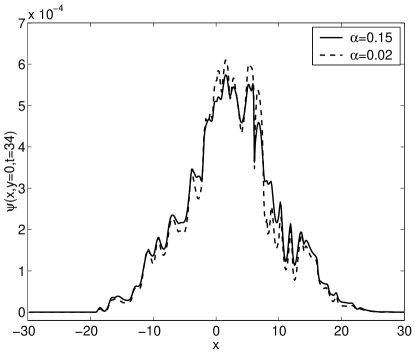
Figure 11: Snapshot of the passive tracer concentration field $\psi(x,y=0)$ for $\mathcal{L}=10^{-2}$ at time $t=34$ for two different values of the filtering parameter $\alpha=0.15$ (solid line) and $\alpha=0.02$ (dashed line).

Second, a local advection orientation, $\Phi(x,y)$, is defined:

$$\cos(\Phi)=\frac{\mathbf{\nabla}\psi\,{\scriptscriptstyle\stackrel{{\scriptstyle\bullet}}{{{}}}}\,\mathbf{u}}{|\mathbf{\nabla}\psi||\mathbf{u}|},$$ (36)

with $\mathbf{u}$ the velocity field. If the local passive tracer concentration is being advected by the local velocity and diffusion is not being sufficiently resolved, then the gradient of the former will be orthogonal to the local velocity, and consequently, $\Phi=\pi/2$. On the other hand, if the local passive tracer concentration exhibits diffusion, then it will change in a direction perpendicular to the local velocity, yielding $\Phi=0$. For small Lewis numbers where the effects of advection dominate over the effects of molecular diffusion, the distribution of the local advection orientation, $P(\Phi)$, over the mid-plane of the cell, should exhibit a strong peak at $\Phi=\pi/2$. This peak will then broaden as the Lewis number is increased, since the effects of diffusion cause the passive tracer concentration to spread out at all orientations relative to the local velocity. The presence of this broadening in the distribution of the local advection orientation is then an indication that molecular diffusion has been sufficiently resolved. The distributions $P(\Phi)$ for the various Lewis numbers ranging from $\mathcal{L}=10^{-4}$ to $\mathcal{L}=10^{-1}$ are plotted in Fig. 12.

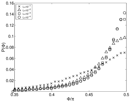
Figure 12: Distribution of local advection orientations for various Lewis numbers ranging from $\mathcal{L}=10^{-4}$ to $\mathcal{L}=10^{-1}$.

The distribution for $\mathcal{L}=10^{-2}$ is distinctly different from that for $\mathcal{L}=10^{-3}$, providing evidence that the molecular diffusion at $\mathcal{L}=10^{-3}$ has been stably resolved, that is, that the chosen grid spacing $\Delta x$ is sufficiently small for the simulation to be accurate. However, the relative similarity in the distributions for $\mathcal{L}=10^{-3}$ and $\mathcal{L}=10^{-4}$ suggests that diffusion for the latter case may not have been sufficiently resolved. Consequently, the smallest allowed Lewis number is set at $\mathcal{L}=10^{-3}$.

References

- Cross and Hohenberg (1994) M. C. Cross and P. C. Hohenberg, Science 263(5153), 1569 (1994).
- Gollub and Cross (2000) J. P. Gollub and M. C. Cross, Nature 404(6779), 710 (2000).
- Hohenberg and Shraiman (1989) P. C. Hohenberg and B. I. Shraiman, Physica D 37, 109 (1989).
- Solomon and Gollub (1988a) T. H. Solomon and J. P. Gollub, Physics of Fluids 31(6), 1372 (1988a).
- Rosenbluth et al. (1987) M. N. Rosenbluth, H. L. Berk, I. Doxas, and W. Horton, Physics of Fluids 30, 2636 (1987).
- Shraiman (1987) B. I. Shraiman, Physical Review A 36(1), 261 (1987).
- McCarty and Horsthemke (1988) P. McCarty and W. Horsthemke, Physical Review A 37, 2112 (1988).
- McLaughlin et al. (1985) D. W. McLaughlin, G. C. Papanicolaou, and O. R. Pironneau, SIAM Journal on Applied Mathematics 45, 780 (1985).
- Busse (1978) F. H. Busse, Reports on Progress in Physics 41, 1929 (1978).
- Solomon and Gollub (1988b) T. H. Solomon and J. P. Gollub, Physical Review A 38, 6280 (1988b).
- Camassa and Wiggins (1991a) R. Camassa and S. Wiggins, Physical Review A 43(2), 774 (1991a).
- Camassa and Wiggins (1991b) R. Camassa and S. Wiggins, Physica D 51, 472 (1991b).
- Ramshankar et al. (1990) R. Ramshankar, D. Berlin, and J. P. Gollub, Physics of Fluids A 2(11), 1955 (1990).
- Ramshankar and Gollub (1991) R. Ramshankar and J. P. Gollub, Physics of Fluids A 3(5), 1344 (1991).
- Solomon et al. (1993) T. H. Solomon, E. R. Weeks, and H. L. Swinney, Physical Review Letters 71(24), 3975 (1993).
- Solomon et al. (1994) T. H. Solomon, E. R. Weeks, and H. L. Swinney, Physica D 76, 70 (1994).
- Cross and Hohenberg (1993) M. C. Cross and P. C. Hohenberg, Review of Modern Physics 65(3), 851 (1993).
- Aref (1983) H. Aref, Journal of Fluid Mechanics 143, 1 (1983).
- Fischer (1997) P. F. Fischer, Journal of Computational Physics 133(1), 84 (1997).
- Chiam et al. (2003) K.-H. Chiam, M. C. Cross, and H. S. Greenside, Physical Review E 67, 056206 (2003).
- Paul et al. (2002) M. R. Paul, M. C. Cross, and P. F. Fischer, Physical Review E 66(4), 046210 (2002).
- Paul et al. (2001) M. R. Paul, M. C. Cross, and P. F. Fischer, Physical Review Letters 87(15), 154501 (2001).
- Paul et al. (2003) M. R. Paul, K.-H. Chiam, M. C. Cross, P. F. Fischer, and H. S. Greenside, Physica D 184, 114 (2003).
- Paul et al. (2004) M. R. Paul, K.-H. Chiam, M. C. Cross, and P. F. Fischer, Physical Review Letters 93(6), 064503 (2004).
- Fletcher (1991) C. A. J. Fletcher, Computational Techniques for Fluid Dynamics, vol. I of Springer Series in Computational Physics (Springer-Verlag, Berlin, 1991), 2nd ed.
- Tannehill et al. (1997) J. C. Tannehill, D. A. Anderson, and R. H. Pletcher, Computational Fluid Mechanics and Heat Transfer (Taylor and Francis, New York, 1997), 2nd ed.
- Fischer and Mullen (2001) P. F. Fischer and J. S. Mullen, Comptes Rendus de l’Académie des Sciences Paris, Série I, Analyse Numérique 332, 265 (2001).
- Bohr et al. (1998) T. Bohr, M. H. Jensen, G. Paladin, and A. Vulpiani, Dynamical Systems Approach to Turbulence (Cambridge University Press, Cambridge, 1998).
- Shlesinger et al. (1995) M. F. Shlesinger, G. M. Zaslavsky, and U. Frisch, eds., Lévy Flights and Related Topics in Physics (Springer, 1995).
- Egolf et al. (1998) D. A. Egolf, I. V. Melnikov, and E. Bodenschatz, Physical Review Letters 80(15), 3228 (1998).