Global Analysis of Synchronization in Coupled Maps

Abstract

We introduce a new method for determining the global stability of synchronization in systems of coupled identical maps. The method is based on the study of invariant measures. Besides the simplest non-trivial example, namely two symmetrically coupled tent maps, we also treat the case of two asymmetrically coupled tent maps as well as a globally coupled network. Our main result is the identification of the precise value of the coupling parameter where the synchronizing and desynchronizing transitions take place.

I Introduction

Although the phenomenon of synchronization of nonlinear oscillators was discovered already in 1665 by Huyghens, it has received systematic attention only recently Pikovsky et al. (2001); Pecora et al. (1997), owing mainly to newly found applications and the understanding of nonlinear systems that we have achieved through modern methods. The field received an impetus after it was discovered by Fujisaka-Yamada Fujisaka and Yamada (1983) and Pikovsky Pikovsky (1984) and further analyzed by Pecora-Carroll Pecora and Carroll (1990) that even chaotic trajectories can synchronize. Since then the phenomenon has found applications in secure communication, coupled Josephson junctions arrays etc. From a completely different perspective, it was observed Eckhorn et al. (1988); Gray et al. (1989) experimentally that synchronous firing of neurons was important in feature binding in neural networks. Distant groups of neurons rapidly synchronize and desynchronize as the input stimulus changes, each synchronized group representing a collection of features belonging to the same percept. Thus a systematic understanding of synchronization and desynchronization has become important in neural information processing Hansel and Sompolinsky (1992); Buzsáki and Draguhn (2004); Friedrich et al. (2004).

As a result of these developments various coupled dynamical systems have been studied that are either continuous or discrete in time, either continuously coupled or pulse coupled etc. and different types of synchronizations have arisen such as phase synchronization or complete synchronization, etc. Coupled maps Kaneko (1993) have been used to a great extent to understand synchronization in particular Gade (1996); Jost and Joy (2002); Jalan and Amritkar (2003); Celka (1996); Chatterjee and Gupte (1996); Maistrenko and Kapitaniak (1996); Balmforth et al. (1999); Gade et al. (1995); Liu et al. (1999); Manrubia and Mikhailov (1999); Sinha (2002) and complexity in dynamical systems Gaspard and Wang (1993); Olbrich et al. (2000); DeMonte et al. (2004) in general. The paradigm here consists of identical individual maps, typically iterates of a functional equation like the logistic one that produce chaotic dynamics. These maps then are coupled, that is each of them computes its next state not only on the basis of its own present state but also on the basis of those other ones that it is coupled to. With appropriate conditions on the coupling strengths, the individual solution is also a solution of the collective dynamics, that is, when all the maps follow their own intrinsic dynamics synchronously, we also have a solution of the coupled dynamics. This is the simplest case of synchronization. That synchronized collective dynamics, however, need not be stable even if the individual ones are. Therefore, the study of synchronization essentially depends on a stability analysis. One may use linear stability analysis or global stability analysis (for some recent formulations, see Pecora and Carroll (1998); Jost and Joy (2002); Chen et al. (2003)). In the linear stability analysis one assumes that the synchronized state follows the same dynamics as the individual uncoupled dynamics and then studies the stability of the dynamics transverse to the synchronizing manifold. However it has been observed Atay et al. (2004) in coupled systems with delays that the synchronized dynamics can be quite different from the individual uncoupled dynamics. Also, it has been demonstrated Ginelli et al. (2002, 2003) that the linear stability analysis can actually fail in a nonlinear setting, due to global nonlinear effects. For a global stability analysis, one has to guess a Lyapunov function which then gives a criterion for synchronization. Thus the linear stability takes only the local dynamics into account and it makes a restricting assumption on the synchronized dynamics. In contrast, the global stability analysis, while global, depends on the choice of the Lyapunov function and may not always give optimal criteria. In general optimal global results are difficult to obtain. In many cases numerical results indicate the global stability of the synchronized state, but it is difficult to prove stability rigorously. Thus it is necessary to develop a method to study synchronization which goes beyond these drawbacks. That is, it should be global and should not make any reference to the synchronized dynamics. This is what we achieve in this paper. We present a new global stability method that leads to sharp results, that is, it can determine the critical value of the coupling parameter above which global synchronization occurs. In order to exhibit the principal features, we first apply the method to the simplest non-trivial case, namely two symmetrically coupled tent maps. Then we consider asymmetric coupling and a globally coupled network.

Our method uses invariant measures or stationary densitiesLasota and Mackey (1994) to study synchronization. A stationary density is the density obtained by starting from some initial distribution of the initial conditions and letting the system evolve for a long time. Though the complete characterization of such densities can be difficult, we shall demonstrate below that it may suffice to study its support to understand synchronization and this can be easier than studying the whole measure. Clearly, this approach is inherently global. The key idea is to study the support of the invariant measure for different coupling strengths and to determine the critical value of the coupling strength when the support shrinks to the synchronized manifold. We consider the following coupled dynamical system

$$X_{n+1}=Af(X_{n})=:S(X_{n})$$ (1)

where $X=(x_{1},x_{2},\cdots,x_{N})^{T}$ is an $N$-dim. column vector, $A$ is an $N\times N$ coupling matrix and $f$ is a map from $\Omega=[0,1]^{N}$ onto itself. As already mentioned, in the present paper we consider the tent map defined as:

$$f(x)=\left\{\begin{array}[]{ll}2x&0\leq x\leq 1/2\\ 2-2x&1/2\leq x\leq 1.\end{array}\right.$$ (4)

Different coupling matrices are chosen.

II Invariant measures

A measure $\mu$ is said to be invariant under a transformation $S$ if $\mu(S^{-1}(A))=\mu(A)$ for any measurable subset $A$ of $\Omega$. For example, a Dirac measure concentrated at a fixed point of the transformation is clearly invariant. An invariant measure need not be unique as can be seen immediately from the fact that if there are several fixed points then the different Dirac measures at these fixed points as well as their linear combinations are all invariant. A natural way to obtain invariant measures is to simply iterate any measure under the transformation $S$ and take an asymptotic (weak-$\star$) limit of these iterates. A sequence $\mu_{n}$ of measures converges in the weak-$\star$ sense to a measure $\mu$ when for all continuous functions $f$ on $\Omega$

$$\lim_{n\to\infty}\int_{\Omega}f(x)\,\mu_{n}(dx)=\int_{\Omega}f(x)\,\mu(dx).$$ (5)

The usefulness of this concept derives from the fact that bounded sets are weak-$\star$ precompact, that is, contain a weak-$\star$ convergent subsequence, see e.g. W.Rudin (1973). In particular, this applies to the dynamical iterates of some initial measure. For example, one may start with any Dirac measure. Our interest, however, is not in such singular measures as they do not sample the whole phase space. We would like to start from a distribution of initial conditions spread over the whole phase space (say uniformly) and study its evolution and what kind of asymptotic limit it leads to. This is the idea of the SRB-measures, as they are called after Sinai, Ruelle, and Bowen. For some dynamical systems, any invariant measure is singular. In such cases even if we start with a uniform density we obtain a singular measure asymptotically. However, if, for example, the map is expanding everywhere then an SRB measure is absolutely continuous w.r.t. to Lebesgue measure. Therefore here we restrict ourselves to one particular map that is expanding, namely the tent map. We want to investigate how such a density depends on the coupling strength and would like to see when its support shrinks to the synchronization manifold.

There are various ways to find invariant measures. One approach is to use the so called Frobenius-Perron operator. It is defined as:

$$\int\int_{D}P\rho(X^{\prime})d^{N}X^{\prime}=\int\int_{S^{-1}(D)}\rho(X^{\prime})dX^{\prime}$$ (6)

If we choose $D=[0,x_{1}]\times\cdots\times[0,x_{N}]$ then we get

$$P\rho(X)=\left({\partial\over\partial x_{1}}\cdots{\partial\over\partial x_{N}}\right)\int\int_{S^{-1}(D)}\rho(X^{\prime})dX^{\prime}$$ (7)

Our $S$ is not invertible. In fact, it has $2^{N}$ disjoint parts. Let us denote them by $S_{i}^{-1}$, $i=1,...,2^{N}$. If $X\in\Omega$, since $f$ is symmetric, we get

$$P\rho(X)=J^{-1}(X)\sum_{i=1}^{2^{N}}\rho(S_{i}^{-1}(X))$$ (8)

where $J^{-1}(X)=|dS^{-1}(X)/dX|$.

III Symmetrically coupled maps

In this section we choose a symmetric dissipative coupling given by

$$A=\left(\begin{array}[]{cc}a-\epsilon&\epsilon\\ \epsilon&a-\epsilon\end{array}\right)$$ (11)

where $0<\epsilon<1$ is the coupling strength and $0<a<1$ is a parameter. This choice for $A$ also satisfies the constraint that the row sum is a constant. This guarantees that the synchronized solution exists.

III.1 The case $a=1$

With this choice of $A$ we get the following functional equation for the density.

$$P\rho(x,y)\!\!\! = \!\!\!{1\over{4|1-2\epsilon|}}[\rho(\beta x/2-\gamma y/2,-\gamma x/2+\beta y/2)$$ (12)

$$\!\!\!+\rho(1-\beta x/2+\gamma y/2,-\gamma x/2+\beta y/2)$$

$$\!\!\!+\rho(\beta x/2-\gamma y/2,1+\gamma x/2-\beta y/2)$$

$$\!\!\!+\rho(1-\beta x/2+\gamma y/2,1+\gamma x/2-\beta y/2)]$$

where $\gamma=\epsilon/1-2\epsilon$ and $\beta=1+\gamma$. Since we know that a point belonging to $\Omega$ does not leave $\Omega$, all the arguments of $\rho$ on the right hand side of the above equation should be between 0 and 1. This gives us four lines $0\leq\beta x/2-\gamma y/2\leq 1$ and $0\leq-\gamma x/2+\beta y/2\leq 1$ which bound an area, say $\Gamma$. The support of the invariant measure should be contained in $\Gamma\cap\Omega$.

Figure 1: The evolution of the support of the invariant measure obtained by starting from the Lebesgue measure supported on the square $[0,1]\times[0,1]$ with $\epsilon<1/4$. a) The parallelogram ABCD obtained after the first application of $A$ b) The rhombus AFIE obtained by applying $f$ to the rectangle ABCD in a. c) The rhombus AFIE one gets when $A$ is applied to the rhombus in b. d) The next application of $f$ leads to the rhombus AMNL.

In order to study the evolution of supp $\rho$ we study the iterates of $\Omega$ under $S=Af$. $f$ maps $\Omega$ onto $\Omega$. Application of $A$ then leads to the parallelogram shown in Fig. 1a. The next application of $f$ leads to Fig. 1b. We use the following convention for labelling the points throughout. A point is labelled by the same letter in its image. As a result, some points in Fig. 1b have two labels. We note that the boundary in Fig. 1b is completely determined by the part of the area in the upper right quadrant in Fig. 1a. This is essentially because $l(GI)>l(EI)$ and $l(HI)>l(FI)$. Let us call this condition A. So the areas in other quadrants get mapped inside the image of this area. Now we operate $A$ again to obtain Fig. 1c and $f$ again to get Fig. 1d. Here we have assumed that $\epsilon$ is sufficiently small so that the $x$-coordinate of F in Fig. 1c is less than 1/2 and by symmetry the $y$-coordinate of E is less than 1/2 (condition B). One can notice that, although the internal structure of the density becomes more complex, the boundary is the same as that in Fig. 1b. Also, by continuing this procedure one can see that the quadrilateral AMNL in Fig. 1d is the support of the density which remains invariant provided $\epsilon$ is sufficiently small.

The coordinates of F are given by

$$\left(\begin{array}[]{cc}1-\epsilon&\epsilon\\ \epsilon&1-\epsilon\end{array}\right)\left(\begin{array}[]{c}\epsilon\over{1-\epsilon}\\ 1\end{array}\right)=\left(\begin{array}[]{c}2\epsilon\\ 1-2\epsilon+2\epsilon^{2}\over{1-\epsilon}\end{array}\right)$$ (19)

As a result, the condition B leads to $\epsilon\leq 1/4$. So when $\epsilon$ satisfies this condition we get the above area as an invariant area. In Pikovsky and Grassberger (1991), Pikovsky and Grassberger have made a similar observation for an asymmetric generalisation of the tent map and later Glendenning Glendinning (2001) has carried forward the analysis mathematically. However there is an important difference between the work in Glendinning (2001) and our work. The aim of the ref. Glendinning (2001) is to study the blowout bifurcation and the Milnor attractor. As a result, there the analysis is restricted to the range of coupling parameters between the blowout bifurcation transition and the complete synchronization transition (this range is absent in the case of the symmetric tent map), whereas we are studying the transition to complete synchronization. We carry out the complete analysis using purely geometric arguments preserving the global nature of the result. In the following two sections we shall also extend the analysis to more general situations.

We remark that the procedure carried out so far is applicable to a general class of nonlinear maps. Thus, by this method, one immediately obtains a value of $\epsilon$ below which there is no synchronization provided one can argue that there exists an absolutely continuous invariant measure. Further discussion of this point is postponed to the concluding section.

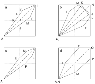
Figure 2: The evolution of the support of the invariant measure obtained by starting from the Lebesgue measure supported on the square $[0,1]\times[0,1]$ with $\epsilon>1/4$. a) The rhombus AFIE obtained by applying $A$ to the rhombus AFIE in Fig. 1b. b) The polygon AEMNLF one gets after the application of $f$ to the rhombus AFIE of a. c) The next application of $A$ transforms the polygon of b to this polygon AEMNLF. d) The new polygon ALOQPM obtained by the next application of $f$ to the polygon in c.

Now we have to check what happens for $\epsilon>1/4$. So we carry out the iterations with this condition in mind. As a result in place of Fig. 1c we obtain Fig. 2a. Now if we apply $f$ we get Fig. 2b. We see that the boundary AEMNLF we obtain now is slightly different from that in Fig. 1d, the corners having been chipped off. The next application of $A$ gives us Fig. 2c. It can be easily checked explicitly that the point E lies on the left and the point M lies on the right of the line $x=1/2$ for any $\epsilon$ greater than $1/4$ . This implies that the boundary obtained by the next application of $f$ (Fig. 2d) looks similar, that is, the number of vertices remains the same. In fact, except for the slanted portions it is exactly the same and we set out to argue that it is indeed different on those small portions. That is we cannot have a set with such a boundary as an invariant area.

In order to do this, let us first note that the magnitude of the slope of any line of the form $y=mx+c$ does not change with $f$ as it scales both axes by the same factor. And $A$ maps such a line to a new line given by

$$y={{\epsilon+(1-\epsilon)m}\over{1-\epsilon+m\epsilon}}x-{{\epsilon c({\epsilon+(1-\epsilon)m)}\over{1-\epsilon+m\epsilon}}}+(1-\epsilon)c$$ (20)

Now if the slanted portion is stable then its slope shouldn’t change under $A$, so we have

$${{\epsilon+(1-\epsilon)m}\over{1-\epsilon+m\epsilon}}=m$$ (21)

This implies $m^{2}=1$ ($m=1$ in our case since we are interested in the region where both coordinates are greater than $1/2$ and $f$ does not change the slope in this region). So the slanted portion in the Fig. 2c, if it is stable, has to be of the form $y=x-(1-2\epsilon)c$. $f$ changes this intercept to $-2(1-2\epsilon)c$ and for it to be stable this should be equal to $-c$ owing to the symmetry. This implies that either $b=0$ or $\epsilon=1/4$. Therefore such a slanted portion cannot be stable for $\epsilon>1/4$ and the whole area cannot be stable either. This shows that $\epsilon_{c}=1/4$ is the critical value below which there exists an invariant area and hence no synchronization. When $\epsilon$ crosses this $\epsilon_{c}$ the area becomes unstable and collapses the synchronization manifold to the line $x=y$ and we get synchronization.

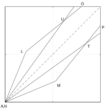
Figure 3: This polygon would be obtained as the support of the evolving measure during the course of iterations if the condition A (see the text) was violated.

If the condition A is violated as well in Fig. 2c during further iterations then in that case the boundary would look something like the one shown in Fig. 3 instead of that in Fig. 2d. But since $\angle MNL>\angle EAF$, there is always a part of nonzero length of the segment $MP$ in Fig. 2c which appears as a boundary in Fig. 3 (segment MT). And then the above argument will apply to this segment.

By symmetry it can be argued that this area again becomes stable if we increase $\epsilon$ further at $\epsilon=3/4$ and this leads to desynchronization. Needless to say that the result agrees with that obtained by the linear stability analysis.

It is interesting to note that the transitions of synchronization and desynchronization are discontinuous in the sense that the area of the support abruptly changes value at the critical thresholds.

Finally, we end this section by making a couple of observations which might be useful in future refinements and/or generalizations of this analysis to other maps. Firstly, it is interesting to note that the vertex $F$ in Fig 1b or c becomes a periodic point of period 2 exactly at $\epsilon=1/4$ and it looses its stability for larger $\epsilon$. Secondly, for $\epsilon<1/4$, the boundary of the invariant area is generated from the boundary of $\Omega$ and hence is stable whereas for $\epsilon>1/4$ there is a small portion of the boundary (segment $EM$ in the Fig. 2 b or c) which does not satisfy this property and becomes unstable.

III.2 The case of general $a$

In this case the synchronized dynamics is different from that of the individual maps. This can be seen by taking the initial point as $X_{0}=(z,z)$ which lies on the synchronization manifold which then leads to the dynamics governed by $X_{n+1}=af(X_{n})$.

Figure 4: The evolution of the support of the measure for the coupling matrix $A$ with general $a$. The iterates are started from the square $[0,1]\times[0,1]$ and $\epsilon<(2a-1)/4$. a) The parallelogram ABCD obtained after the first application of $A$. b) The next application of $f$ transforms the parallelogram in a to this figure.

Now we start the iterations of $\Omega$. The first application of $A$ leads to the Fig. 4a and then $f$ maps it to Fig. 4b. One can see that if $\epsilon$ is sufficiently small so that the point $H$ remains on the left of the line $x=1/2$ after application of $A$ then the $\angle HCG$ remains the same in the subsequent iterations whereas the $\angle FAE$ decreases with the iterations. This leads to the Fig. 5 asymptotically.

Figure 5: The invariant area CHIG obtained asymptotically for the evolution with the coupling matrix $A$ with general $a$.

The above condition on $\epsilon$ can be calculated as for the case $a=1$ and we get $\epsilon\leq(2a-1)/4$. By following similar arguments as for the $a=1$ case it can be shown that this area is unstable for $\epsilon>(2a-1)/4$ and it reduces to the line $x=y$. Again by symmetry it can be seen that the desynchronizing transition will take place at $\epsilon=(2a+1)/4$.

IV Asymmetrically coupled maps

In this section we again choose $N=2$ but now

$$A=\left(\begin{array}[]{cc}1-\epsilon_{1}&\epsilon_{1}\\ \epsilon_{2}&1-\epsilon_{2}\end{array}\right)$$ (24)

where $0<\epsilon_{1},\epsilon_{2}<1$. We write $S(\epsilon_{1},\epsilon_{2})=Af$. We can immediately see that

$$S(\epsilon_{1},\epsilon_{2})\left(\begin{array}[]{c}x\\ y\end{array}\right)=RS(\epsilon_{2},\epsilon_{1})\left(\begin{array}[]{c}y\\ x\end{array}\right),$$ (29)

where

$$R=\left(\begin{array}[]{cc}0&1\\ 1&0\end{array}\right),$$ (32)

i.e., the system remains unchanged under the transformation $\epsilon_{1}\leftrightarrow\epsilon_{2}$ and $x\leftrightarrow y$. This implies that, if $\rho_{\epsilon_{1},\epsilon_{2}}(x,y)$ and $\rho_{\epsilon_{2},\epsilon_{1}}(x,y)$ are the stationary densities generated by $S(\epsilon_{1},\epsilon_{2})$ and $S(\epsilon_{2},\epsilon_{1})$ respectively,

$$\rho_{\epsilon_{1},\epsilon_{2}}(x,y)=\rho_{\epsilon_{2},\epsilon_{1}}(y,x).$$ (33)

As a result, $S(\epsilon_{1},\epsilon_{2})$ and $S(\epsilon_{2},\epsilon_{1})$ synchronize simultaneously when the values of $\epsilon_{1}$ and $\epsilon_{2}$ are varied.

In fact, much more is true. Let us define an operator

$$S_{t}:=S({{\epsilon_{1}+t\epsilon_{2}}\over{1+t}},{{t\epsilon_{1}+\epsilon_{2}}\over{t+1}}) = {{S(\epsilon_{1},\epsilon_{2})+tS(\epsilon_{2},\epsilon_{1})}\over{1+t}}.$$ (34)

In particular $S_{0}=S(\epsilon_{1},\epsilon_{2})$ and $S_{\infty}=S(\epsilon_{2},\epsilon_{1})$. Now it can be seen that $S_{t}X$ lies on a straight line between $S_{0}X$ and $S_{\infty}X$ and all the three points lie on the same side of the line $x=y$. This in particular implies that, for given values of $\epsilon_{1}$ and $\epsilon_{2}$, the boundary of the support of the invariant measure of $S_{t}$ lies between that of $S_{0}X$ and $S_{\infty}X$. In fact, if we define $D\left(\begin{array}[]{c}x\\ y\end{array}\right)=|x-y|$ then we see immediately that $D(S_{t}\left(\begin{array}[]{c}x\\ y\end{array}\right))=|1-\epsilon_{1}-\epsilon_{2}||f(x)-f(y)|$ is independent of $t$ and that, consequently, as $\epsilon_{1}$ and $\epsilon_{2}$ are varied $S_{t}$ synchronizes independently of $t$.

Now when $t=1$ we have $S_{1}=S({{\epsilon_{1}+\epsilon_{2}}\over 2},{{\epsilon_{1}+\epsilon_{2}}\over 2})$ which is symmetric. So we can use the result of the previous section which tells us that the system synchronizes when $\epsilon_{1}+\epsilon_{2}=1/2$ and desynchronizes when $\epsilon_{1}+\epsilon_{2}=3/2$.

It should be noted that the invariant measures generated by $S_{t}$s for different $t$ are not the same. But since we are interested in the synchronization property, i.e., the value of $\epsilon$ at which the support of the measure shrinks to the line $x=y$, we use the identity (34) which gives another equivalent symmetric dynamics. And since this equivalent dynamics is symmetric we know its synchronization properties.

V Globally coupled map network

Now we extend our analysis to a higher dimensional case. We consider a globally coupled network of $N$ maps with all couplings of equal strength. As a result

$$A=\left(\begin{array}[]{cccc}1-\epsilon&\epsilon/(N-1)&\cdots&\epsilon/(N-1)\\ \epsilon/(N-1)&1-\epsilon&\cdots&\epsilon/(N-1)\\ \vdots&\vdots&&\vdots\\ \epsilon/(N-1)&\epsilon/(N-1)&\cdots&1-\epsilon\end{array}\right)$$ (39)

Now we consider the dynamics in the 2-dim space spanned by $\hat{\bf e}_{1}$ and $(1,1,\cdots,1)$. By symmetry this dynamics is the same as that in any other similar subspace, i.e., spanned by $\hat{\bf e}_{i}$ and $(1,1,\cdots,1)$. And all of them synchronize simultaneously. We take the orthogonal vectors $\hat{\bf e}_{1}$ and $(0,1,\cdots,1)$ and a general vector in this space $X=(x,y,y,\cdots,y)^{T}$. Now

$$AX=\left(\begin{array}[]{c}(1-\epsilon)x+\epsilon y\\ {\epsilon\over{N-1}}x+(1-{\epsilon\over{N-1}})y\\ \vdots\\ {\epsilon\over{N-1}}x+(1-{\epsilon\over{N-1}})y\end{array}\right).$$ (44)

As a result, the reduced dynamics of our system in this 2-dim subspace is given by an effective coupling matrix

$$A_{eff}=\left(\begin{array}[]{cc}1-\epsilon&\epsilon\\ {\epsilon\over{N-1}}&(1-{\epsilon\over{N-1}})\end{array}\right)$$ (47)

and from the previous section we know that this dynamics synchronizes when $\epsilon+{\epsilon/(N-1)}=1/2$, i.e., $\epsilon={{N-1}\over{2N}}$. This result again agrees with the one obtained by the linear stability analysis Jalan et al. (2003).

VI Concluding discussion

In this paper we have proposed a method that uses invariant measures and in particular their support to study synchronization. We have demonstrated it on one example, namely the tent map where we were able to study the stability of the support of the invariant measure using purely geometric arguments. In the future, different techniques to deal with invariant measures and their support will have to be developed in order for this method to be of wide use.

We should note that the notion of convergence we have been studying here, namely convergence of the support of the invariant measure as encoded in the convergence of its boundary in general is different from the weak-$\star$ convergence introduced above. That is, there exists the possibility that the measure can become zero asymptotically everywhere except on the synchronization manifold without making the boundary unstable. In other words, the measure can become singular. Here, we have considered the tent map which is expanding everywhere. But it is not sufficient to have the individual map expanding, rather it should be the coupled map that should guarantee the existence of the absolutely continuous measure. In fact, it turns out that, in all the cases considered here, the combined map ceases to be expanding exactly at the synchronization threshold. Clearly this is a consequence of the everywhere expanding property of the map chosen. While this guaranteed for us the existence of the absolutely continuous measure for $\epsilon<\epsilon_{c}$ and validated our use of the present method, it also raises a question as to what happens in the case of other maps. In fact, there exists a considerable activity in Ergodic Theory concerning the existence of an absolutely continuous invariant measures for various discrete dynamical systems (see for example Góra and Boyarsky (1989); Arbieto et al. (2004); Alves (2004)). So for general mappings our approach will have to be complemented by the results in this field.

Other than considering different maps one can also try to apply this method to more complicated connection topologies. Various networks, such as, random, scale-free, small world etc. can be considered. A characterization of complete measures is also needed. We have already taken a step in this direction Jost and Kolwankar (2004). It is important to note that the knowledge of the complete measure was not necessary to study the synchronization since we used only the support of the measure. However, a method to find out that support is the minimum prerequisite for this approach to be useful.