Magic number 7 $\pm$ 2 in networks of threshold dynamics

Abstract

Information processing by random feed-forward networks consisting of units with sigmoidal input-output response is studied by focusing on the dependence of its outputs on the number of parallel paths M. It is found that the system leads to a combination of on/off outputs when $M\lesssim 7$, while for $M\gtrsim 7$, chaotic dynamics arises, resulting in a continuous distribution of outputs. This universality of the critical number $M\sim 7$ is explained by combinatorial explosion, i.e., dominance of factorial over exponential increase. Relevance of the result to the psychological magic number $7\pm 2$ is briefly discussed.

Information processing (IP) in biological systems is often carried out by elements that show threshold-type (sigmoid) input-output (IO) behaviors. For example, the expression of a gene is determined by an on/off-switch for its transcription factors. Another example is the signal transduction system in a cell where the enzymatic reaction often displays a sigmoid output when responding to an external stimulus like the abundance of an input chemicalsignal . One of the most well-studied examples of sigmoid IO relationships can be found in neural networks, where the output of each neuron depends on inputs from other neurons or a receptive field Rosensenblatt .

In these biological networks, the connections among elements are often entangled. Cross-talk in signal transduction has recently been observed for several systemssignal , while enzymatic reactions are generally entangled as well. The connections in neural networks are known to be complex. Besides complexity, biological networks can also display cascade type structures leading from the external input to the final output. In signal transduction such cascades are encountered, while layered networks have been discussed as an idealization of biological neural networks. Hence, the study of entangled layered networks is generally important. The information processing in such systems is discussed by judging whether distinct attracting points (or sets) are reached through the dynamics in successive layers, depending on the input. In a layered network system, e.g., the attracting set is the state of the output layer.

In an entangled network, the more the number of degrees of freedom to be processed increases, the more mutual interference can occur thus increasing the complexity. Consequently, the IP ability of the network depends on the number of processed degrees of freedoms. In this paper, we discuss this number dependence and explore some universal properties of entangled networks with sigmoid units.

In connection with this problem, it is interesting to note that the term magic number $7\pm 2$ was coined in psychology Miller , where the number of chunks (items) that can be memorized in short term memory is found to be limited to about $7\pm 2$. In neural networks, this corresponds to the number of inputs beyond which the output that depends on these inputs no longer clearly separates.

In order to investigate the question raised above, we adopt a cascade perceptron as an abstract model of a random sigmoid responseMcCulloch-Pitts ; Minsky . Here we consider feed-forward network dynamics without feed-back loop, for simplicity. Each layer $l$ is composed of $M$ elements and all elements are regulated by the elements in the preceding layer:

$$x^{l}_{i}=\tanh\left(\frac{\beta}{\sqrt{M}}\sum_{k}^{M}\epsilon^{l}_{ik}x^{l-1}_{k}-\theta^{l}_{i}\right),$$ (1)

where $x^{l}_{i}$ represents the state of the $i$-th element of the $l$-th layer. $\theta^{l}_{i}$ is the threshold value for $x^{l}_{i}$ to be ‘excitatory’. Unless otherwise stated, we set $\theta^{l}_{i}=0$ as this specific choice is not important for the later discussion. The coupling terms $\epsilon^{l}_{ik}$ are chosen randomly from a Gaussian distribution with standard deviation $1.0$. The parameter $\beta$ normalized by $\sqrt{M}$ determines the steepness of the sigmoid function. As $\beta$ approaches $0$, Eq.(1) approaches a constant function with $x^{l}_{i}=0$ (or $x^{l}_{i}=-\theta^{l}_{i}$). On the other hand, as $\beta$ increases, equation (1) approaches a step functions such that in almost all cases $x^{l}_{i}$ becomes either $-1$ or $1$, and each element effectively has just $2$ states. For the medium range of $\beta$, the IO relationship is smooth, which, as will be shown later, may lead to complex dynamics. Note that if all the thresholds $\theta^{l}_{i}=0$, the change of sign $x\to-x$ preserves the equations of the system, so that the solutions for Eq.(1) are symmetric.

For the information processing stages carried out in each layer, $\vec{x}^{l}=F_{l}(\vec{x}^{l-1})$ holds where $\vec{x}^{l}\equiv\left(x^{l}_{1},x^{l}_{2},\cdots,x^{l}_{M}\right)$ and $F_{l}$ is the processing dynamics carried out in the $l$-th layer. We set the values of the $0$-th layer as the inputs to be processed. If a succeeding layer is regarded as a next time step, the present system can be interpreted as a random dynamical systemOtt.PRL where the processing corresponds to temporal evolution. We take various inputs (corresponding to a set of inputs) randomly chosen such that $x^{0}_{i}\in[-1,1]$ for each $i$, and compute numerically the evolution of Eq. (1).

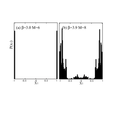
Figure 1: Distribution of $P(x^{l}_{1})$ at layer$l=30$, obtained over $5.0\times 10^{5}$ inputs with a homogeneous distribution over $[-1,1]$. The parameter $\beta=3.0$ and the threshold $\theta$ is set to $0$. The histogram is plotted by using a bin size $2.0/128$. (a) for $M=6$ (b) $M=8$.

Let us first discuss the qualitative behavior of Eq.(1). For $\theta^{l}_{i}=0$, $x^{l}_{i}$ the outputs converge to $0$, irrespectively of the inputs if $\beta<1$, while they approach either $1$ or $-1$ when $\beta$ is large. For middle range values of $\beta$, outputs may take values between -1 and 1, depending on the input. In this regime, outputs are often sensitive to changes of the inputs, and indeed orbital instability exist in the evolution through the layers. The degree of this instability depends on the number of parallel paths and on interference. For sufficiently small $M(\lesssim 7)$, the IP is stable, in the sense that the $x^{l}_{i}$ in the output layer only assume a few distinct values, depending on the input values. On the other hand, if $M$ is large ($\gtrsim 7$), such convergence is not common. We have computed a histogram of the output values $P(x^{l}_{1})$ sampled over $5.0\times 10^{5}$ randomly chosen inputs. As shown in Fig.1, there are clearly two peaks at $x=\pm 1$ for $M=6$ and $P(x)\approx 0$ for $x\neq 1$, while for $M=8$, the distribution is broad.

The scattering in the values $x^{l}_{i}$ of the attractor for the latter case is due to chaotic dynamics in Eq.(1), where stretching and folding in phase space appear note1 . Fig.2(a,b) show values of $x^{l}$ projected onto the $(x^{l}_{1},x^{l}_{2})$ plane. In the plot we take $l=30$ and $10^{5}$ inputs given at $l=0$. For $M=6$(a) each $x^{l}_{i}$ at $l=30$ is localized within a small volume of the total phase space. On the other hand, for $M=8$(b), one can see folding and stretching, and the scattering of points throughout phase space. With these chaotic dynamics, tiny differences in the input values are amplified making clear separation of inputs impossible.

The above simulations are carried out with $\beta=3.0$, but this stretching and folding process is observed as long as $\beta(>1)$. To obtain insight into the dependence on $\beta$, values of $x^{l=30}_{1}$ for 800 inputs are plotted as a function of $\beta$ in Fig.3. For $M=6$, they converge to a few points for a large portion of $\beta$, while for (b) $M=8$ they do not.

These numerical results suggest that a critical number of parallel paths $M_{c}$ exists, beyond which chaotic dynamics is inevitable, and that $M_{C}$ is around $7$ for a wide range of $\beta$. We confirm this critical number by computing several characteristic quantities for the model Eq.(1).

First, we plot the fraction of bins for which $P(x^{l}_{1})$ is not zero in each layer in Fig.4(a). Here $P(x^{l}_{1})$ is computed over $5.0\times 10^{5}$ inputs, by taking a bin size of $2.0/128$. For $M\leq 7$ the fraction becomes smaller from layer to layer, while for $M\geq 8$ the fraction is almost one and does not decrease much for successive layers. For $M\leq 7$, the output points are well separated by the sigmoid function, while they are scattered over the whole range of values $[-1,1]$ for $M\geq 8$. The data for Fig.4(a) are obtained for a fixed threshold $\theta_{i}=0$, but the conclusion does not change even when the thresholds are distributed, as shown in Fig.4(b) where $\theta_{i}\in[0,0.5]$. These behaviors are also invariant against changes in $\beta$, as long as it is sufficiently larger than 1 but not that large for the $\tanh$ function to effectively become a step function. Hence the critical number $M_{c}\approx 7$ is rather general, without dependencies on the details of the model.

Second, we have computed the degree of orbital instability in the chaotic dynamics, i.e., the sensitivity on input values. By regarding a layer as a time step in a dynamical system, the sensitivity is computed by the Lyapunov exponent of the random map Eq.(1) as followsstability :

$$\lambda_{max}=\max_{\vec{x},|\vec{x}|=1}\frac{1}{l}\ln|J^{l}J^{l-1}\cdots J^{1}\vec{x}|$$ (2)

where $J^{l}$ is the Jacobian matrix of Eq.(1), $J^{l}_{ik}\equiv\frac{\partial x^{l}_{i}}{\partial x^{l-1}_{k}}$, so that $\delta x^{l}_{j}=\sum_{k}J^{l}_{ik}(x^{l-1})~{}\delta x^{l-1}_{k}$. The fraction of the network having positive exponents $\lambda_{max}$ is plotted in Fig.5 for the following three cases: $\theta^{l}_{i}=0$ with a Gaussian distribution for $\epsilon^{l}_{ik}$, $\theta^{l}_{i}=0$ with a uniform distribution for $\epsilon^{l}_{ik}\in[-1,1]$, and distributed thresholds $\theta_{ij}\in[0,0.5]$ with a Gaussian distribution for $\epsilon^{l}_{ik}$. For all of the three cases, the fraction of networks with chaotic behavior drastically increases around $M=7$.

Loss of separability of inputs around the number 7 due to chaotic dynamics is not limited to the model investigated above. We have also investigated some other models consisting of units with threshold dynamics (of Michaelis-Menten’s form for enzymatic reactions), that are randomly connected in a cascadeIshiharaKaneko . The same behavior with the same critical number 7 is obtained. On the other hand, it is also interesting to note that Milnor attractors that collide with their basin boundary are dominant for globally coupled dynamical systems with more than $7\pm 2$ degrees of freedomKK-Milnor ; KK-magic7 .

Then, why is the critical number $7$ (or $7\pm 2$) so universal? In KK-magic7 , one of the authors(KK) discussed the possibility that the combinatorial explosion of the basin boundaries due to chaotic dynamics is relevant to this critical number (i.e., the faster increase of $N!$ over $2^{N}$). This combinatorial argument can be extended to the present problem.

We do so by considering the origin of the folding process. In order to see the effect of entanglement, we study the input-output relationship of $x^{0}_{1}\rightarrow x^{2}_{1}$ of a two-layer systemnote2 by fixing the inputs of $x^{0}_{2},\cdots,x^{0}_{M}$. Then output $x^{2}_{1}$ is given as a function of $x^{0}_{1}$; $x^{2}_{1}=\tanh(\sum_{j}\sigma_{j}(x^{0}_{1}-\nu_{j}))$ where $\sigma_{j}(u)=\tilde{\beta}\epsilon^{2}_{1j}\tanh(\tilde{\beta}\epsilon^{1}_{j1}u)$ and $\nu_{j}=(\epsilon^{l}_{j1})^{-1}\sum_{k=2}^{M}\epsilon^{1}_{jk}x^{0}_{k}$. Here it is assumed that $\tilde{\beta}\equiv\beta/\sqrt{M}$ is large, and that $tanh(x)$ is close to a step function. Note that there are $N$ paths via the middle layer elements where $x^{1}_{j}$ switches between the values -1 and 1 as $x^{0}_{1}$ crosses the ‘threshold’ $\nu_{j}$. One can then renumber the index $j=1,\cdots,M$ such that $-1<\nu_{1}<\nu_{2}<\cdots<\nu_{M}<1$. With this ordering, if $\sigma_{j}$ is positive and $\sigma_{j+1}$ is negative, the one-dimensional mapping $x^{0}_{1}\rightarrow x^{2}_{1}$ has a single hump at $\nu_{j}<x<\nu_{j+1}$ implying a folding process as in the logistic map. Then, if the sign of $\sigma_{j}$ alternates for successive $j$, the above function switches between $-1$ and $1$ at $\nu_{j}$ $M$ times as $x^{0}_{1}$ is increased;  The one-dimensional mapping from the input $x^{0}_{1}$ to the output $x^{2}_{1}$ is thus subject to this folding process everywhere in $-1<x<1$. Since $\epsilon^{2}_{1j}$ can take positive or negative values with equal probability, the probability to have full folding decreases proportionally to $2^{-M}$.

The estimate given so far is for fixed inputs of $x_{2},x_{3},\cdots,x_{M}$. By changing these input values, the ordering of $\nu_{j}$ changes accordingly (for the original index without reordering) and hence there are in total $(M-1)!$ possible orderings. Therefore, roughly speaking, the input-output relationship has full up-down switches for some input values $x_{2},x_{3},\cdots,x_{M}$, when $(M-1)!2^{-M}$ exceeds $1$. In this case, at every layer, for any element, the folding occurs fully for some inputs, and the folding process covers most of phase space. Even though this argument is quite rough, it is still possible to presume that when $(M-1)!$ exceeds the order of $2^{M}$, the chaotic dynamics replaces the separation by the threshold function. Note that this factorial surpasses $2^{M}$ at $M=6$ coinciding with the magic number $7\pm 2$. This could be the reason why at the magic number $7\pm 2$, the separation of states collapses and chaotic dynamics takes over.

In the present paper, we have shown that the interference between inputs drastically increases around $M\sim 7$ within the general setup of neural networks. The argument of magic number $7\pm 2$ presented here is only based on combinatorial arguments, and does not strongly depend on the choice of parameters. Hence it is naturally expected that our explanation works for a wide class of entangled cascade networks with sigmoid units. Considering also the generality of the mechanism, it is not particularly far fetched to infer a correspondence between our result and the original magic number $7\pm 2$ in psychology. Of course, at present the underlying neurodynamics associated with the actual psychological process is still unknown, and hence we do not claim that we have found the solution to the magic number 7 problemTsudaNicolis . Nevertheless, the formation of distinct attracting sets resulting from inputs channeled through layered networks with sigmoidal elements is common among neural processes, and hence it is important to mention the connection.

The authors are grateful to K. Fujimoto, T. Shibata and F. H. Willeboordse for discussion. This work was supported by a Grant-in-Aid for Scientific Research from the Ministry of Education, Science, and Culture of Japan (11CE2006).

Figure 2: Snapshots of $(x_{1}^{l},x_{2}^{l})$ at layer $l=30$, plotted as a projection of $\vec{x}^{l}$ on to the two dimensional plane $(x_{1},x_{2})$. The data obtained from $10^{5}$ randomly chosen inputs are overlaid with $\beta=3.0$. (a) $M=6$. The density of points is quite high around $(\pm 1,\pm 1)$. (b) $M=8$. Multiple folding and stretching processes are detected, while the points are scattered over the plane.

Figure 3: Bifurcation diagram of $x^{l=30}_{1}$ against $\beta$. $x^{l}_{1}$ at layer $l=30$ is plotted over $800$ different inputs for each $\beta$. For $\beta(\lesssim 1.0)$, $x^{l}$ converge to $x_{1}=0$. (a) $M=6$. For most inputs, $x^{l=30}_{1}$ converges to $\pm 1$ if $\beta$ is sufficiently larger than $1$. (b) for $M=8$, $x^{l=30}_{1}$ is scattered over $[-1,1]$.

Figure 4: The average fraction of the value $x$ such that $P(x^{l}_{1}=x)>0$, plotted as a function of $M$. The histogram is computed for $10^{5}$ inputs over $200$ networks (i.e., with different choices of $\epsilon^{l}_{ik}$), with a bin size $2.0/128$. The fraction at layer $l=10,20,30,40,50$ is plotted. (a) with threshold $\theta^{l}_{i}=0$ and (b) with distributed threshold $\theta_{i}\in[0,0.5]$. The parameter $\beta$ is fixed at $3.0$.

Figure 5: The ratio of networks which shows ‘chaotic’ behavior for some values of $\beta$, plotted as a function of $M$. $500$ networks are chosen for $\epsilon^{l}_{ik}$. The Lyapunov exponent is computed by using $J^{l}$ over 500 steps (layers). The behavior is judged numerically as ”chaotic” if the exponent is larger than $0.0$. The ratio is computed for the following three cases; the threshold $\theta^{l}_{i}=0$ with a Gaussian distribution of $\epsilon^{l}_{ik}$ (cross); distributed thresholds $\theta_{ij}\in[0,0.5]$ with a Gaussian distribution of $\epsilon^{l}_{ik}$  (box);and $\theta^{l}_{i}=0$ with a uniform distribution for $\epsilon^{l}_{ik}\in[-1,1]$ (circle).

References

- (1) B. D. Gomperts, I. M. Kramer and P. E. R. Tatham Signal Transduction (Academic Press Inc., 2002).
- (2) F. Rosensenblatt, Principle of Neurodynamics (Spartan 1961).
- (3) G. A. Miller, The psychology of communication (Basi Books, N.Y., 1975).
- (4) W. Pitts and W. S. McCulloch, Bull. Math. Biol. 9 127 (1947).
- (5) M. L. Minsky and S. A. Rapert, Perceptrons expanded edition (The MIT Press, 1988).
- (6) L. Yu, E. Ott, and Q. Chen, Phys. Rev. Lett. 65 2935 (1990).
- (7) From a dynamical systems point of view, the above process is similar to Ott.PRL where a change of the parameter value makes the effective maximum Lyapunov exponent be positive.
- (8) From this Jacobi matrix, the linear stability of the state, for the case with is calculated. This leads to the stability condition for , where is a polyGamma functionrand-mat .
- (9) A. Crisanti, G.Paladin, A. Vulpiani Products of Random Matrices (Springer-Verlag, 1992).
- (10) S. Ishihara and K. Kaneko, to be published
- (11) K. Kaneko, Phys. Rev. E 66 055201(R) (2002).
- (12) K. Kaneko, Phys. Rev. Lett. 78 2736 (1997); Physica D 124 322. (1998).
- (13) M. Timme, F. Wolf,and T. Geisel, Phys. Rev. Lett. 89 154105-1 (2002).
- (14) The folding cannot occur in a single layer because the present system separates the output set linearly, as is well known. At least two layers are necessary for a folding processes.
- (15) J. S. Nicolis and I. Tsuda, Bull. Math. Biol. 47 343 (1985) discussed the magic number in psychology, in relationship with dynamical systems.