]http://www.cp.cmc.osaka-u.ac.jp/ tokita

Species Abundance Patterns in Complex Evolutionary Dynamics

Abstract

An analytic theory of species abundance patterns (SAPs) in biological networks is presented. The theory is based on multispecies replicator dynamics equivalent to the Lotka-Volterra equation, with diverse interspecies interactions. Various SAPs observed in nature are derived from a single parameter. The abundance distribution is formed like a widely observed left-skewed lognormal distribution. As the model has a general form, the result can be applied to similar patterns in other complex biological networks, e.g. gene expression.

If we investigate the number and populations of species in an ecosystem, we can observe universal characteristic patterns in that ecosystem. How to clarify the mechanisms underlying those species abundance patterns (SAPs) has been one of the ’unanswered questions in ecology in the last century May (1999)’ even though the knowledge obtained from it would affect vast areas of nature conservation. Various models have been applied to ecosystem communities where species compete for niches on a trophic level Motomura (1932); Corbet et al. (1943); MacArthur (1960); Preston (1962); Whittaker (1970); Bazzaz (1975); May (1975); Sugihara (1980); Nee et al. (1991); Tokeshi (1999); Hubbel (2001); Hall et al. (2002); McGill (2003); Volkov et al. (2003); Pigolotti et al. (2004), but these models have left the more complex systems a mystery. Such systems occur on multiple trophic levels and include various types of interspecies interactions, such as prey-predator relationships, mutualism, competition, and detritus food chains. Although SAPs are observed universally in nature, their essential parameters have not been fully clarified.

I consider, then, a widely adopted model of biological networks represented by the so-called $N$-species replicator equation (RE) Hofbauer and Sigmund (1998);

$$\frac{{\rm d}x_{i}}{{\rm d}t}=x_{i}\left(\sum_{j}^{N}J_{ij}x_{j}-\frac{1}{N}\sum_{j,k}^{N}J_{jk}x_{j}x_{k}\right)_{,}$$ (1)

to calculate the abundance $x_{i}(t)(\in[0,N])$ of species $i(=1,2\ldots,N)$. Here we assume that $(J_{ij})$ is a time-independent random symmetric $(J_{ij}=J_{ji})$ matrix whose elements have a normal distribution with mean $m(>0)$ and variance $\tilde{J}^{2}/N$ as

$$P(J_{ij})=\sqrt{\frac{N}{2\pi\tilde{J}^{2}}}\exp\left[-\left(\frac{N}{2\tilde{J}^{2}}\right)\left(J_{ij}-m\right)^{2}\right]_{.}$$ (2)

Self-interactions are all set to a negative constant as $J_{ii}=-u(<0)$. Note that the essential parameter is unique as $p\equiv(u+m)/\tilde{J}$ because the transformation of the interaction $K_{ij}\equiv(J_{ij}-m)/\tilde{J}$ does not change the trajectory of the dynamics (1). Although ecologists do not generally believe in the randomness of interspecies interactions in nature, the discipline has been affected by the random interaction model May (1972) as a prototype of complex systems.

The RE appears in various fields Hofbauer and Sigmund (1998). In sociobiology, it is a game dynamical equation for the evolution of behavioral phenotypes; in macromolecular evolution, it is the basis of autocatalytic reaction networks (hypercycles); and in population genetics it is the continuous-time selection equation in the symmetric $(J_{ij}=J_{ji})$ case. The symmetric RE also corresponds to a classical model of competitive community for resourcesMacArthur and Levins (1967).

Particularly in the context of ecology, the $N-1$ species Lotka-Volterra (LV) equation

$$\frac{{\rm d}y_{i}}{{\rm d}t}=y_{i}\left(r_{i}-\sum_{j}^{N-1}b_{ij}y_{j}\right)$$ (3)

is equivalent to the $N$ species RE Hofbauer and Sigmund (1998). That is, the abundance $y_{i}$ and the parameters in the corresponding LV are described by those in the present RE model as,

$$y_{i}=x_{i}/x_{M}\quad(i=1,2,\ldots,N)$$ (4)

$$r_{i}=J_{iM}-J_{MM}=J_{iM}+u$$ (5)

$$b_{ij}=J_{ij}-J_{Mj}$$ (6)

where the ’resource’ species $M\,(y_{M}=1)$ can be arbitrarily chosen from $N$ species in the RE. The ecological interspecies interactions $(b_{ij})(i\neq j)$ have a normal distribution with mean $0$ and variance $2\tilde{J}^{2}/N$ from Eq. (6), and they are no longer symmetric ($b_{ij}\neq b_{ji}$). The present model therefore describes an ecological community with complex prey-predator interactions $((b_{ij},b_{ji})\to(+,-)\,\mbox{or}\,(-,+))$, mutualism $(+,+)$ and competition $(-,-)$. Moreover, a community can have a ’loop’ (detritus) food chain $((b_{ij},b_{ji})\to(+,-),(b_{jk},b_{kj})\to(+,-),(b_{ki},b_{ik})\to(+,-))$. The intraspecific interaction $b_{ii}$ turns out to be related to the intrinsic growth rate $r_{i}$ as $b_{ii}=J_{ii}-J_{Mi}=-u-J_{iM}=-r_{i}$ and is therefore competitive $(b_{ii}<0)$ for producers $(r_{i}>0)$ or mutualistic $(b_{ii}>0)$ for consumers $(r_{i}<0)$.

By Eq. (5), the intrinsic growth rates also have a normal distribution with mean $u+m$ and variance $\tilde{J}^{2}/N$. The probability at which $r_{i}$ is positive–that is, that the $i$-th species is a producer–is therefore given by the error function,

$$\mbox{Prob}(r_{i}>0)=\int_{-p\sqrt{N/2}}^{\infty}\frac{{\rm d}t}{\sqrt{\pi}}\exp\left(-t^{2}\right)_{.}$$ (7)

Consequently, the parameter $p$ can be termed as the ’productivity’ of a community because the larger the $p$, the greater the number of producers. The parameter $p$ is also connected to the maturity of an ecosystem because $m$ increases in time in an evolutionary model Tokita and Yasutomi (2003).

The symmetry $(J_{ij}=J_{ji})$ makes the average fitness $\bar{f}\equiv\sum_{j,k}^{N}J_{jk}x_{j}x_{k}$ (the second term of the r.h.s. of Eq. (1)) a Lyapunov function Hofbauer and Sigmund (1998), which is a nondecreasing function of time in dynamics (1). Therefore, every initial state converges to a local maximum of $\bar{f}$ as $t\to\infty$. Interpreting ${\mathcal{H}}\equiv-\frac{1}{2}\bar{f}$ as an energy function, we can study macroscopic functions like free energy at such a maximum by using the technique of statistical mechanics of random systems Mezard et al. (1987); Diederich and Opper (1989); Biscari and Parisi (1995); de Oliveira and Fontanari (2000, 2001, 2002).

Information on equilibrium states of dynamics (1) at $t\to\infty$ is derived from the zero-temperature limit of free energy density,

$$f \equiv -\lim_{\beta\to\infty}\lim_{N\to\infty}\frac{1}{N\beta}\left[\ln Z\right]_{J}$$ (8)

$$Z \equiv \int_{0}^{\infty}\left(\prod_{i}^{N}{\rm d}x_{i}\right)\delta(N-\sum_{k}^{N}x_{k}){\rm e}^{-\beta{\mathcal{H}}}$$ (9)

where $\left[\ldots\right]_{J}\equiv\int_{-\infty}^{\infty}{\rm d}J_{ij}P(J_{ij})(\ldots)$ denotes the ’sample average Mezard et al. (1987)’ over random interactions. The Dirac delta function in Eq. (9) reflects the conservation of total abundance $\sum_{i}^{N}x_{i}(t)=N$ satisfied at any $t$ in Eq. (1). The calculation of Eq. (8) is similar to calculations in the previous works Diederich and Opper (1989); Biscari and Parisi (1995); de Oliveira and Fontanari (2000, 2001, 2002) and yields mean field equations for the order parameters $q$ and $v$ as

$$p-v=\sqrt{q}\int_{-\Delta}^{\infty}(z+\Delta){\rm D}z$$ (10)

$$(p-v)^{2}=\int_{-\Delta}^{\infty}(z+\Delta)^{2}{\rm D}z$$ (11)

where $\Delta\equiv\sqrt{q}(p-2v)$ and ${\rm D}z\equiv{\rm d}z\exp(-z^{2}/2)/\sqrt{2\pi}$. The resulting equations turn out to be formally the same as the case where $m=0$ and $\tilde{J}=1$ Diederich and Opper (1989). For each value of $p$, Eqs. (10) and (11) are solved numerically.

Among macroscopic functions calculated in the present framework, the most significant for a theory of SAPs is the survival function $\alpha_{p}(x)\equiv\frac{1}{N}\sum_{i}^{N}\theta(x_{i}-x)$, the proportion of species whose abundance is larger than $x$, where $\theta(z)(=1(z>0);0(z\leq 0))$ is the step function. Similar to the fashion in which free energy was calculated, the survival function $\alpha_{p}(x)$ is analytically calculated and represented by the order parameters as

$$\alpha_{p}(x) \equiv \lim_{\beta\to\infty}\lim_{N\to\infty}\left[\int_{0}^{\infty}\left(\prod_{j}^{N}{\rm d}x_{j}\right)\right.$$ (12)

$$\left.\,\times\;\theta(x_{i}-x)\delta\left(N-\sum_{k}^{N}x_{k}\right)\frac{\exp(-\beta{\mathcal{H}})}{Z}\right]_{J}$$

$$\!\!\!\!\!\!\!\!\!\!\!\!=\alpha_{p}(0)\tilde{\theta}(x)-\int_{-\Delta}^{\infty}\tilde{\theta}\left(x-\frac{\sqrt{q}(z+\Delta)}{p-v}\right){\rm D}z$$

where the definition of the step function above is given by $\tilde{\theta}(z)=1(z\geq 0);0(z<0))$.

The resulting function $\alpha_{p}(0)\equiv v(p-v)$ and $\alpha_{p}(1)$ of $p$ can be termed ’diversity’, i.e., the proportion of nonextinct species and that of the species with abundance larger than unity, respectively, as depicted in Fig. 1. This demonstrates a typical positive correlation between productivity and diversity Waide and et al (1999). Numerical results for $\alpha_{p}(1)$ are also depicted in Fig. 1 for comparison. We see good agreement between the analytical and the numerical results for $p\gtrsim 1$, while some deviations appear for small values of $p$. This small-value deviation is attributable to the occurrence of replica symmetry breaking (RSB)Mezard et al. (1987); Biscari and Parisi (1995) for $p<\sqrt{2}$, which yields a number of metastable states of Eq. (8), and the replicator dynamics (1) essentially converges to not only a ground state of (8) but also to the metastable states. Since the energy ${\mathcal{H}}$ and the diversity are both nonincreasing functions of time in dynamics (1), the mean-field results here give a lower minimum of diversity. Interestingly, the metastable states enhance the diversity. The analysis of RSB is expected to improve the quantitative agreement Biscari and Parisi (1995).

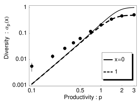
Figure 1: Diversity $\alpha_{p}(x=0,1)$ as a function of $p$ of log-log scales. Black circles show numerical solutions of $\alpha_{p}(1)$ averaged over $50$ samples of $(J_{ij})$ for Eq. (1) with $N=2048$ and $p=0.1,0.2,0.3,0.4,0.5,\sqrt{2}/2,1,\sqrt{2},2,3$. Error bars indicate the maximum and minimum values found in the samples.

Note that $\alpha_{p}(x)$ is also represented as a function of species rank $n$:

$$\alpha_{p}(x)=\frac{n}{N}\quad\mbox{for}\quad x\in[x^{(n+1)},x^{(n)})_{,}$$ (13)

$(n=1,2,\ldots,S\leq N)$ if the species abundance is ranked in descending order, as in $x^{(1)}\geq x^{(2)}\geq\cdots\geq x^{(n)}\geq\cdots\geq x^{(S)}>0$. As the function $\alpha_{p}(x)$ is a nonincreasing monotonic function, the species abundance relation, i.e., the abundance $x^{(n)}$ as a function of a rank $n$, is given by the inverse function of $\alpha_{p}(x)$ as $x^{(n)}=x_{p}(n/N)=\alpha_{p}^{(-1)}(x)$, depicted in Fig. 2 for some values of $p$. We observe two typical SAPs in different regions Hubbel (2001) and with different species compositions Whittaker (1970): one is a straight line like the geometric series Motomura (1932) for a small value of $p$, and the other consists of sigmoid curves on a logarithmic vertical axis for some range of $p$. This latter SAP denotes a lognormal-like abundance distribution. Remarkably, the transition of the SAPs from low $p$ to high is identical to the observed transition from low- to high-productivity areas; that is, from a species-poor area such as an alpine or polar region to a species-rich tropical rain forest Hubbel (2001). The transition also corresponds to the secular variation of SAPs observed in abandoned cultivated land Bazzaz (1975). This supports the contention that $p\;(\mbox{or}\,m)$ is a maturity parameter, as is suggested by an evolutionary model Tokita and Yasutomi (2003).

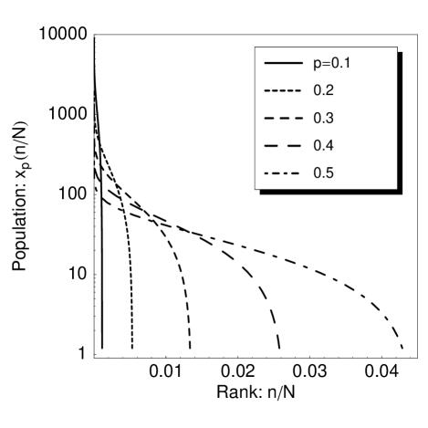
Figure 2: Rank-abundance relations as a function of productivity $p$ on normal-log scales.

The abundance distribution is also derived from the survival function. As $C_{p}(x)\equiv 1-\alpha_{p}(x)$ is a cumulative distribution function of abundance, the abundance distribution is given by the derivative $F_{p}(x)\equiv{\rm d}C_{p}(x)/{\rm d}x$ and

$$F_{p}(x) = \frac{p-v}{\sqrt{2\pi q}}\exp\left\{-\frac{(p-v)^{2}}{2q}\left(x-\frac{q(p-2v)}{p-v}\right)^{2}\right\}$$ (14)

$$\,+\,\,C_{p}(0)\delta(x)$$

where the second term denotes the rate of species extinction. The first term is a normal distribution but not a lognormal distribution. Nevertheless, the curves in Fig. 2 demonstrate a typical sigmoid pattern on a logarithmic vertical axis. This pattern indicates the coexistence of very abundant species with rare ones. This multiscale of abundance is intuitively understood by a divergent behavior of the variance $\sigma^{2}\equiv q/(p-v)^{2}$ of $F_{p}(x)$ for small $p$ because $q\to\infty$ and $v\to 0$ for $p\to 0$. Moreover, the mode of $F_{p}(x)$ per ’natural’ octave Preston (1962) $\ln(x)$ is always a positive value (as shown in Fig. 3) at $x^{*}=\frac{\sigma}{2}(\Delta+\sqrt{\Delta^{2}+4})>0$, which denotes a unimodal distribution. Indeed, the mode diverges as

$$x^{*}\to\frac{\sigma}{|\Delta|}=\frac{1}{(p-v)|p-2v|}\to\infty$$ (15)

for $p\to 0$. As a result, the abundance distribution is a truncated normal distribution with a large variance $\sigma^{2}\to\infty$ and a negatively divergent mean $\mu\equiv\frac{q(p-2v)}{p-v}\to-\infty$ satisfying $\frac{\sigma}{\mu}=\frac{1}{\Delta}\to 0$ for $p\to 0$. This is why the abundance distribution per octave looks like a left-skewed lognormal distribution Nee et al. (1991) in Fig. 3.

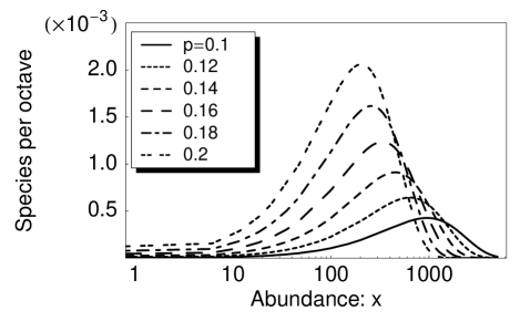
Figure 3: Abundance distribution per ’natural’ octave $\ln(x)$. Functions $F_{p}(x)x({\rm d}(\ln(x))=F_{p}(x){\rm d}x)$ for some values of $p$ are depicted, whereas Preston originally defined octaves as logarithms to base 2 Preston (1962).

Moreover, we derive an analytical expression for the population $x_{max}$ of the most abundant species, the position of the individual curve mode $x_{N}$, and therefore the ratio of their logarithm defined as $\gamma\equiv\log(x_{N})/\log(x_{max})$. According to the canonical hypothesis Preston (1962); May (1975), the parameter $\gamma$ takes a value near unity in various real communities. To check the validity of the canonical hypothesis, we first need to evaluate an expected value of the most abundant species $x_{max}$. From the definition of $x_{max}$, that is $NF_{p}(x_{max})=1$, and the conservation of the total abundance $\int_{0}^{\infty}F_{p}(x)x{\rm d}x=N$, which is equivalent to $\sum_{i}^{N}x_{i}=N$, we obtain

$$x_{max}=\frac{q(p-v)+\sigma\sqrt{2\ln\left(\frac{\sigma(1-\alpha_{p}(0))+\Delta\alpha_{p}(0)}{\sqrt{2\pi}}\right)}}{p-v}_{.}$$ (16)

On the other hand, the mode of the individual curve $F_{p}(x)x$ per octave is given by $x_{N}=\frac{\sigma}{2}\left(\Delta+\sqrt{\Delta^{2}+8}\right)$, and finally, the parameter $\gamma\equiv\log(x_{N})/\log(x_{max})$ is evaluated by substituting the values of the order parameters $q$ and $v$ for each value of $p$. In the present model, $\gamma$ is a monotonically increasing function of $p$ and $0.96<\gamma<1.04$ for $0.1<p<0.6$, denoting that the canonical hypothesis is supported in the range of $p$ giving the typical SAPs in Fig. 3. Although the canonical hypothesis was demonstrated to be merely a mathematical consequence of lognormal distribution May (1975) rather than anything biological, it is noteworthy that the lognormal-like abundance distribution with $\gamma\simeq 1$ derives from basic ecological dynamics. This still suggests a biological foundation for the hypothesis in a large complex ecosystem, in the same way that a biological foundation was indicated for the theory of a local competitive community Sugihara (1980).

In the present model, all species coexist only in the limit $p\to\infty$, that is, in the trivial cases in which interspecies interactions are negligible ($\tilde{J}\ll u$ ) or homogeneous ($\tilde{J}\to 0$), thereby giving $\alpha_{\infty}(x)=\theta(1-x)$, $x^{(n)}=x_{\infty}(n/N)=1$ for all $n$ and $F_{\infty}(x)=\delta(x-1)$.

The present theory seeks to capture the influence of productivity on the SAPs under the assumption that all species interact randomly; nevertheless, this assumption itself is never justified because it ignores a biological correlation between interactions produced by evolution. However, note that the randomness is assumed only for an initial state with $N$ species in Eq. (1). Actually, the simulation reveals the resulting interactions of nonextinct species to be nonrandom: every sample for $p\in[0.1,3]$ in Fig. 1 evolves to only flora, $\forall i\,\,r_{i}>0$. Moreover, by ordering species as $r_{i}>r_{j}$ for any $i<j$, we observe a hierarchy: there are only three types of interactions, that is, mutualism $(b_{ij},b_{ji})=(+,+)$, competition $(-,-)$ and exploitation of $i$ on $j$ as $(+,-)$, but no reverse $(-,+)$. This suggests the applicability of the present model to a plant community.

It has been demonstrated that empirically supported patterns are derived from a single parameter of general population dynamics. This not only suggests the importance of globally coupled biological interactions in a large assemblage but also provides a unified viewpoint on mechanisms of similar patterns observed in other biological networks with complex interactions; for example, a lognormal abundance distribution of a protein in cells Blake et al. (2003); Kaneko (2003); Sato et al. (2003), which is revealed by gene expression networks.