Isotropic third-order statistics in turbulence with helicity: the 2/15-law

Abstract

The so-called 2/15-law for two-point, third-order velocity statistics in isotropic turbulence with helicity is computed for the first time from a direct numerical simulation of the Navier-Stokes equations in a $512^{3}$ periodic domain. This law is a statement of helicity conservation in the inertial range, analogous to the benchmark Kolmogorov 4/5-law for energy conservation in high-Reynolds number turbulence. The appropriately normalized parity-breaking statistics, when measured in an arbitrary direction in the flow, disagree with the theoretical value of 2/15 predicted for isotropic turbulence. They are highly anisotropic and variable and remain so over a long times. We employ a recently developed technique to average over many directions and so recover the statistically isotropic component of the flow. The angle-averaged statistics achieve the 2/15 factor to within about $7\%$ instantaneously and about $5\%$ on average over time. The inertial- and viscous-range behavior of the helicity-dependent statistics and consequently the helicity flux, which appear in the 2/15-law, are shown to be more anisotropic and intermittent than the corresponding energy-dependent reflection-symmetric structure functions, and the energy flux, which appear in the 4/5-law. This suggests that the Kolmogorov assumption of local isotropy at high Reynolds numbers needs to be modified for the helicity-dependent statistics investigated here.

1 Introduction

There are two invariants of the inviscid Navier-Stokes equations – the total energy, defined by $E=\frac{1}{2}\int{\bf u}({\bf x})^{2}d{\bf x}$, and the total helicity $H=\int{\bf u}({\bf x})\cdot\boldsymbol{\omega}({\bf x})d{\bf x}$ where the vorticity $\boldsymbol{\omega}({\bf x})=\nabla\times{\bf u}({\bf x})$. Energy has been extensively studied especially in statistical theories of turbulence as well as in experiments. Helicity, being sign-indefinite has been more challenging to study theoretically. Direct experimental measurements of helicity are also difficult because of the need to measure local gradients, requiring high resolution and careful probe design (see for example Kholmyansky et al. (2001)). Nevertheless, since the discovery of helicity as a conserved quantity by Moreau (1961) and independently by Moffat (1969), there have been several attempts to draw parallels with the energy dynamics. The existence of a helicity cascade was proposed by Brissaud et al. (1973) and various possible inertial range scalings of the energy and helicity spectra were discussed. The joint forward (downscale) cascade of energy and helicity has been verified in direct numerical simulations, most recently by Chen et al. (2003a). A recent work by Kurien et al. (2004), showed that there is a relevant timescale for helicity transfer in wavenumber space. The proper consideration of the helicity flux timescale showed that helicity can modify the energy dynamics, measureably slowing it down in the high wavenumbers.

We here present a study of the small-scale phenomenology of turbulence with helicity in the manner of the Kolmogorov (1941) investigation (K41) of helicity-free turbulence. Using the Kármán-Howarth equation for the dynamics of the second-order two-point correlation function (see von Kármán & Howarth (1938)), K41 gives the benchmark 4/5 energy law for homogeneous, isotropic, reflection-symmetric (helicity-free) turbulence, assuming finite mean energy dissipation $\varepsilon$ as $\nu\rightarrow 0$,

$$\langle(u_{L}({\bf x}+{\bf r})-u_{L}({\bf x}))^{3}\rangle=-\frac{4}{5}\varepsilon r$$ (1)

for $\eta\ll r\ll L_{0}$, the so-called inertial range. See Eyink & Sreenivasan (2004) for a recently discovered derivation of a similar law by Onsager. $\eta$ is the Kolmogorov dissipation scale, $L_{0}$ is the typical large scale, $u_{L}({\bf x})={\bf u}({\bf x})\cdot{\hat{\bf r}}$ is the longitudinal component of ${\bf u}$ along ${\hat{\bf r}}$, the mean energy flux in the inertial range equals the mean dissipation rate $\varepsilon=2\nu\langle|\nabla{\bf u}|^{2}\rangle$, and $\langle\cdot\rangle$ denotes an ensemble average of a high-Reynolds number decaying flow. It has been shown empirically and proved that this is equivalent to a long-time average in statistically steady high-Reynolds number turbulence (Frisch (1995)). The 4/5-law is a statement of the conservation of energy in the inertial range scales – the third-order structure function is an indirect measure of the flux of energy through scales of size $r$. A key assumption of the K41 theory was ‘local isotropy’ or isotropy of the small scales $r\ll L_{0}$ at sufficiently high Reynolds number. This assumption appears to hold according to high Reynolds number experimental measurements of the 4/5-law even when the data are acquired in only a single direction in the flow (Sreenivasan & Dhruva (1998)).

Recently, a local version of the K41 statistical laws were proved in Duchon & Robert (2000) (see also Eyink (2003) for the case of the 4/5-law in particular): Given $any$ local region $B$ of size $R$ of the flow, for $r\ll R$, and in the limits $\nu\rightarrow 0$, next $r\rightarrow 0$, and finally $\delta\rightarrow 0$,

$$\langle(\Delta u_{L})^{3}\rangle_{(\Omega,B)} = \lim_{\delta\rightarrow 0}\frac{1}{\delta}\int^{t+\delta}_{t}d\tau\int\frac{d\Omega}{4\pi}\int_{B}\frac{d{\bf x}}{R^{3}}[\Delta u_{L}({\bf r};{\bf x},\tau)]^{3}=-\frac{4}{5}\varepsilon_{B}r.$$ (2)

for almost every (Lebesgue) point $t$ in time, where $\Delta u_{L}({\bf r})=u_{L}({\bf x}+{\bf r})-u_{L}({\bf x})$ and $\varepsilon_{B}$ is the instantaneous mean energy dissipation rate over the local region $B$. The angle integration $d\Omega$ integrates in ${\bf r}$ over the sphere of radius $r$. For each point ${\bf x}$ the vector increment ${\bf r}$ is allowed to vary over all angles and the resulting longitudinal moments are integrated. The integration over ${\bf x}$ is over the flow subdomain $B$. This version of the K41 result does not require isotropy, homogeneity, long-time or ensemble averages, or stationarity of the flow. This version of the 4/5-law has not yet been rigorously verified empirically. It was shown by Taylor et al. (2003) that at the very least, the 4/5-law does not seem to require isotropy, long-time or ensemble averaging; it appears to be sufficient to average over many angles and over the domain at any instant of a sufficiently ‘high’ Reynolds number flow.

The first attempt to study the symmetry and dynamics of the two-point correlation function in flows with helicity was made by Betchov (1961). The simplest symmetry breaking of a statistically rotationally invariant flow is to break parity (mirror-symmetry) by the introduction of helicity. A useful analogy which we borrow from Betchov (1961) is of a well-mixed box of screws. This is statistically invariant to rigid rotations, that is it is isotropic. But under reflection in a mirror all the left-handed screws become right-handed and vice-versa, that is the system is parity- or mirror-symmetry breaking. In particular, no combination of rigid rotations can transform the box of screws into its reflected image. This is the type of symmetry breaking we are considering here. Analogous to the K41 4/5-law, the so-called $2/15$-law for homogeneous, isotropic turbulence with helicity was derived by Chkhetiani (1996) (see also L’vov et al. (1997) and Kurien (2003)),

$$\langle\Delta u_{L}({\bf r})(u_{T}({\bf x}+{\bf r})\times u_{T}({\bf x}))\rangle=\frac{2}{15}hr^{2}$$ (3)

where the transverse component of the velocity $u_{T}({\bf x})={\bf u}({\bf x})-u_{L}({\bf x})$; the mean helicity flux which equals the mean helicity dissipation rate in steady state is $h=2\nu\langle(\partial_{j}u_{i})(\partial_{j}\omega_{i})\rangle$, where the vorticity $\boldsymbol{\omega}=\nabla\times{\bf u}$. We shall use the notation

$$H_{LTT}({\bf r})=\langle\Delta u_{L}({\bf x})(u_{T}({\bf x}+{\bf r})\times u_{T}({\bf x}))\rangle$$ (4)

to denote the third-order helical statistics. The quantity $H_{LTT}({\bf r})$ is the simplest third-order velocity correlation which can have a spatially isotropic component while at the same time displaying a ‘handedness’ due to the cross-product in its definition. $H_{LTT}({\bf r})/r^{2}$ is a measure of the helicity flux through scales of size $r$ in the inertial range which must balance the helicity dissipation $h$ in the viscous range for statistically steady turbulence. The 2/15-law assumes inertial-range behavior of helicity in some range of scales $\eta\ll r\ll L_{0}$. A shell model calculation by Biferale et al. (1998) has demonstrated the likelihood of the 2/15-law. However it has not been measured in experiments or, until the present work, in direct numerical simulations of the Navier-Stokes equations.

Theoretically, the 2/15-law has been shown to apply to the case of high-Reynolds number decaying flows; the arguments for the forced case have not yet been developed. In our initial investigation into the 2/15-law statistics for decaying flows with prescribed isotropic helicity and energy spectra (see Polifke & Shtilman (1989)), we were able to observe some of the qualitative features of the flow but the Reynolds numbers achievable for given our computing abilities was insufficient to observe the 2/15-law. We therefore moved to perform forced simulations to achieve higher Reynolds numbers and to use the statistically steady state to compute the statistics.

In the next section describes the simulations and the calculation of the statistical quantities of interest for the 2/15-law. We present a comparison with the 4/5-law calculation of the same flow, highlighting the differences between energy and helicity dynamics. We show that in the inertial range the helicity flux is more anisotropic and intermittent than the energy flux; and that the smallest resolved scales show recovery of isotropy for energy-dependent statistics but show persistent anisotropy for helicity-dependent statistics over the 10 large-eddy turnover times for which simulation ran. We will conclude with some final remarks on what our analysis means for future work in the area of helicity dynamics and parity-breaking in turbulent flows.

2 Simulations and Results

$N$	$\nu$	$R_{\lambda}$	$E$	$\varepsilon$	$H$	$h$	$k_{\rm max}\eta$
512	$10^{-4}$	270	1.72	1.51	-26.8	62.2	1.1

Table 1: Parameters of the numerical simulation. $\nu$ - viscosity; $R_{\lambda}$ - Taylor Reynolds number; mean total energy $E=\frac{1}{2}\sum_{k}\tilde{\bf u}({\bf k})^{2}$; $\varepsilon$ - mean energy dissipation rate; mean total helicity $H=\sum_{k}\tilde{\bf u}({\bf k})\cdot\tilde{\boldsymbol{\omega}}({\bf k})$; $h$ - mean helicity dissipation rate; Kolmogorov dissipation scale $\eta=(\nu^{3}/\varepsilon)^{3/4}$.

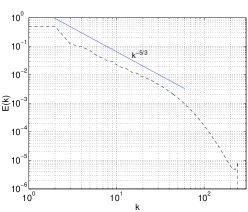
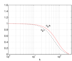
Figure 1: Left panel: Dashed line – Energy spectrum as a function of wavenumber. Solid line – Line of slope -5/3 on the log-log scale. Right panel: Dashed line – Flux of energy $\Pi_{E}$ normalized by mean dissipation rate of energy $\varepsilon$. Solid line – Flux of helicity $\Pi_{H}$ normalized by mean dissipation rate of helicity $h$.

We performed a simulation of the forced Navier-Stokes equation in a unit-periodic box with $512$ grid points to a side. In these units the wavenumber $k$ is in integer multiples of 2$\pi$. The forcing scheme was the deterministic forcing of Taylor et al. (2003), modeled after the deterministic forcing used in Chen et al. (2003a). This forcing simply relaxes the Fourier coefficients in the first two wave numbers so that the energy matches a prescibed target spectrum $F(k)=0.5$ ($k=1,2$). The forcing does not change the phases of the coefficients, which are observed to change slowly in time. In addition, maximum helicity was injected into the wavenumbers 1 and 2 using the scheme of Polifke & Shtilman (1989). The calculation ran for 10 large-eddy turnover times. The flow achieved steady state in about 1 large-eddy turnover time. The statistics reported here have been calculated over a total of 45 frames spanning the latter 9 eddy turnover times. The same data were reported in Kurien et al. (2004). Some additional parameters of the simulation are given in Table 1. The left panel of Fig. 1 shows the mean energy spectrum with a line indicating the Kolmogorov $k^{-5/3}$ scaling and (see Kurien et al. (2004) for the interpretation of the deviation from $k^{-5/3}$ at the high end of the inertial range) The right panel of Fig. 1 shows helicity fluxes normalized by the mean energy and helicity dissipation rates respectively. Note the close to decade range of wavenumbers where $\varepsilon$ and $h$ match the energy and helicity fluxes respectively very well.

2.1 Third-order helical velocity statistics and the use of angle-averaging

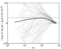
(a) $\widetilde{H}_{LTT}({\bf r})$ in 73 different directions of the flow (dotted lines) from a single frame after the flow has reached statistically steady state. The thick solid line is the mean over all the directions.

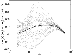
(b) The time-average of $\widetilde{H}_{LTT}({\bf r})$ in each of the 73 different directions (dotted lines) and of the angle-average (thick solid line).

Figure 2: Instantaneous and time-averaged 2/15 law calculations. The 2/15 value is indicated by the horizontal line in both plots. The inertial range is roughly estimated to be $30<r/\eta<150$. Note that the vertical scale in the two plots is not the same; the time-averaged quantities on the right have reduced spread compared to the instantaneous quantities on the left.

We first define the compensated quantity

$$\widetilde{H}_{LTT}({\bf r})=H_{LTT}({\bf r})/(h~{}r^{2}).$$ (5)

In Fig. 2(a) we show $\widetilde{H}_{LTT}({\bf r})$ calculated from a single frame arbitrarily chosen after the flow achieved statistically steady state. Each dotted line is $\widetilde{H}_{LTT}({\bf r})$ in one of 73 different directions in the flow, as a function of scale size $r$. The directions are fairly uniformly distributed over the sphere (see Taylor et al. (2003) for how these directions were chosen). None of the curves show a tendency towards the theoretically predicted $2/15=0.1$3̇ value for an extended range of scales. Among the calculations shown are those for the three coordinate directions which are the most often reported in statistical turbulence studies. For any given $r$ the different directions yield vastly different values. Exceptional are the very largest (forced) scales where the different directions appear to converge. This already signals something different than the usual expectation that anisotropy, if any, should come from, and dominate in, the large scales. The anisotropy persists strongly into the smallest resolved scales, as seen in the large spread of values among the different directions at $r/\eta\approx 2$, where we might expect viscous effects are important. Indeed it appears that it would be fortuitous for the statistics in an arbitrary direction to yield the correct theoretical prediction for isotropic flow.

Next we extract the isotropic component of these statistics using the angle-averaging technique of Taylor et al. (2003). The resulting angle-independent contribution is the thick solid curve in Fig. 2(a). Its peak value is $\approx 0.124$, within 7% of the 2/15 value. While individual directions are both parity-breaking as well as anisotropic, the angle-averaged value recovers the isotropic component of the parity-breaking features (recall the analogy to the box of screws in Section 1). This is a remarkable result out of a single snapshot; there is no $a$ $priori$ reason to expect that angle-averaging an arbitrarily chosen, highly anisotropic snapshot, will yield consistency with the 2/15-law which was derived for isotropic flow. We believe that this result is strong motivation for the existence of a local 2/15 law analogous to the local 4/5-law of Eyink (2003),

$$\langle\Delta u_{L}({\bf r})(u_{T}({\bf x}+{\bf r})\times u_{T}({\bf x}))\rangle_{(\Omega,B)} = \lim_{\delta\rightarrow 0}\frac{1}{\delta}\int^{t+\delta}_{t}d\tau\int\frac{d\Omega}{4\pi}\int_{B}\frac{d{\bf x}}{R^{3}}$$ (6)

$$\times [\Delta u_{L}({\bf r};{\bf x},\tau)][(u_{T}({\bf x}+{\bf r})\times u_{T}({\bf x}))]$$

$$= \frac{2}{15}h_{B}r^{2}.$$

where $\Omega$, $B$, $R$ and $t$ have the same meanings as for Eq. (2); $h_{B}$ denotes the locally (in space and time) averaged helicity dissipation rate. We emphasize that there is as yet no proof for Eq. (6); we have merely written down a conjecture by analogy to Eq. (2), motivated by the calculations for a single snapshot of the flow.

To check if the anisotropy observed in a single frame persists over time, we averaged $\widetilde{H}_{LTT}({\bf r})$ in each of the 73 different directions over 9 large-eddy turnover times (45 frames). We performed the same time-average for the angle-average. The result is shown in Fig. 2(b). The spread in the inertial-range decreased by about a factor of 2 while the spread in the smallest scales decreased by a factor of about 6 relative to the single-frame statistics of Fig. 2(a).

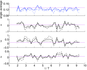
Figure 3: $\widetilde{H}_{LTT}({\bf r})$ for various inertial range values of $r/\eta$ as a function of number of eddy turnover times. $r/\eta=30$ (dashed line), $r/\eta=65$ (solid line), $r/\eta=120$ (dotted line). From top to bottom: Angle-averaged, x-direction, y-direction, z-direction. Note that the vertical scales in the four panels are not the same; the bottom three panels corresponding to the coordinate directions have a much greater spread of values than the top panel for the angle-average. The mean and standard deviations for the $r/\eta=65$ (middle of the inertial range) in each case are given in Table 2.

Inertial range	2/15-law	4/5-law
Theory	0.133̇	0.8
Angle-avg	0.126 $\pm$ 0.009	0.75 $\pm$ 0.03
x	0.02 $\pm$ 0.31	0.78 $\pm$ 0.14
y	0.26 $\pm$ 0.23	0.75 $\pm$ 0.13
z	0.14 $\pm$ 0.21	0.76 $\pm$ 0.11

Table 2: Mean and standard deviation of the compensated third order statistics in the middle of the inertial range.

Inspite of this, the residual variance is significant as we demonstrate in Fig. 3 and as compared below to the same analysis done for the 4/5-law. We plot a time-trace of the angle-averaged $\widetilde{H}_{LTT}(r)$ in the top panel of Fig. 3 for $r/\eta=30$ (lower end of the inertial range), $r/\eta=65$ (middle of the inertial range) and $r/\eta=120$ (higher end of the inertial range). The angle-averaged value in the middle of the inertial range ($r/\eta=65$) is 0.126$\pm$0.009, within error of the predicted value of 2/15 $=$ 0.13̇. The value ranges from $0.119$ and $0.126$ across the inertial range with variances of $8-9\%$. This puts the mean angle-averaged value within 1.5 standard deviations of the theoretical value of 2/15 across the inertial range. Since most prior numerical simulations investigations have studied two-point statistics in the coordinate directions only, we present in the bottom three panels of Fig. 3, the values of $\widetilde{H}_{LTT}({\bf r})$ again at various values of $r/\eta$ for ${\bf{\hat{r}}}$ in the $x$-, $y$- and $z$-directions respectively as a function of time. Table 2 (column 2) shows the mean and standard deviation for each of the four time-trace plots of Fig. 3 in the middle of the inertial range at $r/\eta=65$. The first thing to notice is that none of the coordinate directions average to $2/15$ over long times. This behavior demonstrates that these statistics are highly anisotropic and remain so over long times. Secondly, the mean values in the coordinate directions are poorly defined and practically meaningless in the sense of having extremely large standard deviations. In turbulence phenomenology, such large jumps in values from their mean is the signature of intermittency–the presence of strong, anomalous events. We conclude that the helicity flux in a particular direction is highly intermittent in the inertial range (see Chen et al. (2003b) for a different approach to this issue).

We return briefly to one of the subtleties of the 2/15-law, namely that it was derived for decaying flows. Our initial tests of the 2/15-law in ensemble averages over decaying flows with prescribed initial isotropic helicity and energy spectra (see Polifke & Shtilman (1989) for the method) showed qualitatively the same results. That is, the large anisotropy among the different directions and their intermittency is similar to the forced case reported here and their angle-average has the same qualitative behavior indicating some constant flux in the middle of the range and smoothly approaching zero as $r\rightarrow 0$ (see Fig. 4).

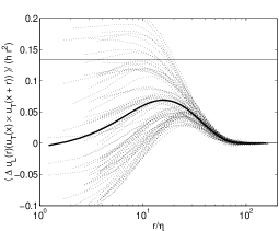
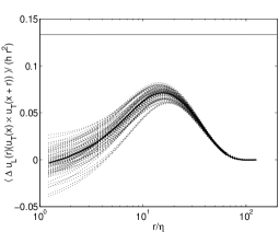
Figure 4: Instantaneous (left-panel) and ensemble-averaged (right-panel), calculations of $\widetilde{H}_{LTT}({\bf r})$ for the test decaying case at $256^{3}$ ($R_{\lambda}\sim 50$). The initial energy and helicity spectra were isotropic with helicity in all the modes. The snapshot is from when the flow had maximally developed and the ensemble average is over 30 such realizations with random phases for each realization. The 2/15 value is indicated by the horizontal line in both plots. Note the qualitative similarity to the forced case of Fig. 2 especially in the small scales ($r<20$). The 2/15 value is not attained, presumably due to the low Reynolds number.

However the Taylor Reynolds numbers achieved were too low (O(50)) to see the 2/15 value which is our primary interest in this investigation. Our computational resources restrict us to forced turbulence when investigating high-Reynolds number effects. Given the qualitative similarities in the data, we anticipate that a careful analysis for the forced case would give the same result as for the decaying case.

2.2 Comparative analysis of the 4/5-law

We compare these results with the analogous ones for the 4/5-law for the same flow. As before, we define the compensated third-order longitudinal structure function

$$\widetilde{S}_{L,3}({\bf r})=\langle(u_{L}({\bf x}+{\bf r})-u_{L}({\bf x}))^{3}\rangle/(\varepsilon r).$$ (7)

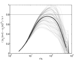
(a) $\widetilde{S}_{L,3}({\bf r})$ in 73 different directions of the flow (dotted lines) from an arbitrarily chosen frame after the flow has achieved statistical equilibrium. The thick solid line is the mean over all the directions.

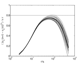
(b) The time-average of $\widetilde{S}_{L,3}({\bf r})$ in each of the 73 different directions (dotted lines) and of the angle-average (thick solid line).

Figure 5: Instantaneous and time-averaged calculations of the 4/5-law. The 4/5 value is indicated by the horizontal line in both plots.

Figure 5(a) shows a single frame calculation of $\widetilde{S}_{L,3}({\bf r})$ for 73 different directions as a function of $r$ (dotted lines). We performed the angle-averaging exactly as in Taylor et al. (2003) to recover the isotropic mean (thick solid line). Our first observation is that the 4/5-law is recovered in this helical flow to as good a degree as in the simulation with zero mean helicity of Taylor et al. (2003). This demonstrates that the reflection-symmetry assumption of Kolmogorov need not hold in order to see this result. This is understood by the fact that the lowest-order (unclosed) dynamical equations for the symmetric second-order correlation functions (von Kármán & Howarth (1938)) from which the 4/5-law was derived by Kolmogorov (1941), decouple from their antisymmetric counterpart (Betchov (1961)) from which the 2/15-law was derived. The third-order longitudinal structure functions of the K41 law are reflection-symmetric by definition, and therefore cannot directly probe the helical, parity-breaking properties of the flow; while the third-order correlation function $H_{LTT}$, cannot probe the reflection-symmetric properties of the flow. The 4/5- and 2/15-laws in fact coexist in turbulent flows with helicity. This possibility was first hinted at by Betchov (1961), who noted that in the equations of motion of statistical moments, the fourth-order correlation function dynamics are the lowest order at which coupling of the symmetric (energy-dependent) and antisymmetric (helicity-dependent) quantities can occur.

In Fig. 5(b) the time-averaged compensated third-order longitudinal structure function for all the directions converge rather well relative to the single frame in Fig. 5(a) in the inertial range. There is still significant spread of values among the different directions in the inertial range but it is far less than in the time-averaged 2/15-law calculation in Fig. 2(b). To make a more quantitative comparison, we present the mid-inertial-range values of the angle-averaged, and the $x$-, $y-$ and $z-$direction calculations in Table 2, column 3. The time mean for the angle-average is well-defined at $0.75\pm 0.03$, a small standard deviation of 4$\%$. The means in the coordinate directions range from $0.75$ to $0.78$, not intolerably far from the $0.8$ value expected from theory, but with significant standard deviation in time of the order of 20$\%$. Still, the behavior is very different from the 2/15-law statistics (Table 2, column 2), where not only was the 2/15 value not achieved in an arbitrary direction, but the variability in time was huge, 100% or more. We are lead to conclude that in the inertial range, both instantaneously and over long times, the helicity flux (as described by the 2/15-law) is far more anisotropic and intermittent than the energy flux (as described by the 4/5-law) for the same statistically steady flow.

2.3 The viscous range

Anisotropy of $\widetilde{H}_{LTT}$ persists into the smallest resolved scales as demonstrated by the large variance among the directions in the range $r/\eta<10$ in Figs. 2(a) and  2(b). By contrast, the angular-dependence of $\widetilde{S}_{L,3}({\bf r})$ becomes very small in the same range in a snapshot (Fig. 5(a)) and even more so on average over time (Fig. 5(b)). In these scales the 2/15- and 4/5-laws no longer hold as viscous effects become important; the quantities $\widetilde{H}_{LTT}$ and $\widetilde{S}_{L,3}$ no longer correspond strictly to the helicity and energy fluxes respectively. The viscous terms for the symmetric quantities, interpreted as energy dissipation at scales $r\approx\eta$, are strictly a sink for energy, pulling energy out of the flow. As is well known, the viscous terms for the antisymmetric quantities, correspondingly the helicity-dissipation at scales $r\approx\eta$, may be positive (producing helicity) or negative (removing helicity). Nevertheless, if the small scale statistics $H_{LTT}$ are to be isotropic, the different directions might be expected to converge in the very small scales. In Table 3, column 2, we show time-mean and standard deviation of the angle-average and the $x$-, $y$- and $z$-direction calculations of $H_{LTT}({\bf r})$ at $r/\eta\approx 2$. The time-mean angle-averaged value is about 0.014 $\pm$ 0.004, a standard deviation of about $30\%$. As in the inertial range, the time-mean in a particular direction does not agree with the angle-averaged value and the standard deviations are enormous. We have shown the corresponding numbers for the 4/5-law for comparison (Table 3, column 3); the means in a particular direction agree better with the angle-averaged mean, and the variances are around 5%, indicating recovery of isotropy in the small-scales and relatively weaker intermittency than for the 2/15-law statistics. We here introduce a note of caution about the results in the viscous range as our simulation is only resolved upto $r/\eta\approx 2$ ($k_{\rm max}/\eta\approx 1.1$). While the inertial range is amply resolved, the viscous range might display some residual effects of being under-resolved. Nevertheless, to the extent that in the $same$ flow, the energy-dependent statistics recover isotropy rather quickly in the viscous scales, it seems worthwhile to note that the helicity-dependent statistics remain dramatically and persistently anisotropic in the viscous scales over the long duration of our simulation.

Viscous range	2/15-law	4/5-law
Angle-avg	0.014 $\pm$ 0.004	0.035 $\pm$ 0.006
x	-0.05 $\pm$ 0.65	0.057 $\pm$ 0.004
y	0.02 $\pm$ 0.57	0.055 $\pm$ 0.003
z	0.17 $\pm$ 0.55	0.057 $\pm$ 0.003

Table 3: Mean and standard deviation of the compensated third order statistics for the smallest resolved scale.

3 Conclusions

This analysis shows that the statistically steady state (forced turbulence) as well as $local$ versions of the 2/15-law analogous to the forced (Frisch (1995) and local 4/5-law (Eyink (2003)), might hold true; we hope our empirical results motivate a theoretical effort towards the proofs. The helicity flux is significantly more anisotropic and intermittent than the energy flux. This suggests that the viscous generation and dissipation of helicity in the small scales is highly anisotropic as well. This might be related to the strong helical events seen in the transverse alignment of vortices in the work of Holm & Kerr (2002). There is an underlying isotropic component of the flow which is extracted by the angle-averaging procedure of Taylor et al. (2003). It is not surprising that angle-averaging recovers the orientation-independent component of the field. However it is remarkable that this spherically averaged value tends to the predicted 4/5 and 2/15 values for $\widetilde{S}_{L,3}$ and $\widetilde{H}_{LTT}$ respectively. This suggests that the ’local isotropy’ requirement of K41 may be relaxed in favor of a hypothesis that the flow statistics have a universal underlying isotropic component.

We conclude with two remarks which were not explicitly mentioned in the body of this paper. The issues of anisotropy and intermittency of the small-scales of the flow are intimately connected with the particular kind of statistics measured. We have shown that in the same flow, certain statistics which depend on energy flux recover isotropy in the small scales, while others which depend on helicity do not. It is therefore more sensible to speak of isotropy (or lack of isotropy) of the $statistics$ of the flow rather than of the flow itself. A second relevant remark is that our numerical data and analysis give some indication as to what might be expected when measuring $H_{LTT}({\bf r})$ in high-Reynolds number experimental flows. In many such experiments, data is acquired at a few points over long times, and the statistics are obtained by applying Taylor’s hypothesis to obtain the spatial correlations in a single-direction (for example, the streamwise direction in a windtunnel). Assuming there is some helicity in the flow, it might not be possible to predict the behavior of $H_{LTT}({\bf r})$ for a particular direction ${\bf\hat{r}}$ (see Kholmyansky et al. (2001)). In this respect, the full-field information and angle-averaging technique appear to be $fundamental$ to recovering the 2/15 isotropic prediction. An experimental effort such as the three-dimensional velocity field imaging of Tao et al. (2002) might be needed to see the $2/15$-law experimentally. This is very different from measurement of the 4/5-law for energy, where, given Reynolds number high enough, the statistics in any direction are observed to recover isotropy in the small scales.