Dynamics of inhomogeneous one–dimensional coupled map lattices

Abstract

We study the dynamics of one–dimensional discrete models of one–component active medium built up of spatially inhomogeneous chains of diffusively coupled piecewise linear maps. The nonhomogeneities (“defects”) are treated in terms of parameter difference in the corresponding maps. Two types of space defects are considered: periodic and localized. We elaborate analytic approach to obtain the regions with the qualitatively different behaviour in the parametric space. For the model with space–periodic nonhomogeneities we found an exact boundary separating the regions of regular and chaotic dynamics. For the chain with a unique (localized) defect the numerical estimate is given. The effect of the nonhomegeneity on the global dynamics of the system is analyzed.

and

1 Introduction

One of the effective methods of analysis of several systems is based on their representation by discrete models. For this one can use the space discretization as well as the time one. Using the space discretization the initial (continuous) system is modelled by a finite set of elements that are coupled according to some rules, which follows from the nature of the system of interest. Each element of these then occurs to be some (small) dynamical system which may be described by a (small) set of dynamical variables. If the time is also discretized, i.e. if the evolution of these dynamical subsystems is considered at discrete time–steps, then such subsystems are treated as maps. In this case spatio-tempotal models are said to be lattice of coupled maps.

The examples of application of the space–time discretization in studies of the nonlinear media are numerous. Here we mention the problems related to chaos and noise in distributed systems [1, 2, 3, 4], to description of the excitable media [4, 5] and some other similar problems (see e.g. [6, 7, 8, 9, 10, 11, 12, 13, 14] and references therein). Moreover, any numerical analysis of a continuous system has in fact to be reduced to the study of space–time discretized model.

In principle, a variety of different space–time lattices may be used. The mostly studied are the models where only the nearest–neighbour (local) coupling is taken into account (see e.g. [8, 9, 10, 12, 13] and references therein). In other models the global coupling, i.e. when all elements of the system are coupled with each other, is assumed [15, 16, 17]. In lattices with the local coupling, as a rule, this is considered as a diffusional one [1, 2, 4, 8, 9, 10, 11, 12, 13]. Mainly, these models are used to analyse the spatio–temporal chaos, pattern formation, self–organization phenomena, etc. [18, 19, 20]

If all the elements are the same, then such lattices are called homogeneous. If, however, elements are different, then the lattice is not a homogeneous one, and its investigation is much more complex. With applied point of view the nonhomegeneity may be two–fold: either elements of the system have different maps, or they have functionally identical maps but with different control parameters. The nonhomogeneities are usually said to be defects. The relative position of defects may vary from a single localized inclusion to a space–periodic ordering.

In most of studies of coupled map lattices, the case of homogeneous lattices (and mainly numerically) has been addressed. However, it is clear, that the assumption of the homogeneity is a crude simplification. Therefore it is rather important to investigate the sensitivity of the lattice dynamics to certain nonhomogeneities (see, e.g., [21, 31] and references therein).

The present study is devoted to the spatially inhomogeneous 1D lattices (in fact, chains) of diffusively coupled piecewise–linear maps, which refer to some models of the one–dimensional excitable media [22]. The defects are determined as maps with different parameter values. Using the exact calculation of the Lyapunov exponents we analyse the behaviour of the lattice with a localized defect and with the space–periodic nonhomegeneity. We also describe the structure of the phase space of such systems.

2 Models of spatially inhomogeneous excitable media

Here we consider the dynamics of two models of inhomogeneous active media: one–dimensional (annular) chain of coupled maps with periodic nonhomegeneity and with one localized defect. To introduce the notations, we remind that the term “map” is implied transformation of some interval $I$ on itself: $T_{a}:I\longrightarrow I$, where $I=[\alpha,\beta]\in{\bf R}^{1}$, $x\mapsto G(x,a)$, $x\in I$, $G(x,a)$ is some function and $a$ is a parameter. In terms of iterations $k$ this may be written as $x(k+1)=G(x(k),a)$, $x\in I$. The nonhomegeneity means nonuniformity of the parameter $a$ along the chain of maps. The functions $G$ are chosen in such a way that they model the one–component active medium.

2.1 Homogeneous medium

Consider the system of $N$ diffusively coupled maps

$$x_{n}(k+1)=G(x_{n}(k),\alpha,\gamma)+\varepsilon\Bigl{(}x_{n+1}(k)-2x_{n}(k)+x_{n-1}(k)\Bigr{)}$$ (1)

with periodic boundary conditions, $x_{n+N}(k){\equiv}x_{n}(k)$, where $n=1,2,\ldots,N$ being the discrete space coordinate, $k=0,1,2,\ldots$ is the discrete time, $\varepsilon>0$ is the (constant) diffusion coefficient, and $\alpha>0$, $\gamma$ are the parameters of the map. This choice of the coupling means that the spatial and temporal actions in map (1) occur simultaneously. Let $G$ be the piecewise linear function:

$$G(x,\alpha,\gamma)=x+\alpha F(x)-\gamma=\cases{(1-2\alpha)x-\gamma,&$x<1/2$;\cr\ &$\ $\cr(1-2\alpha)x-\gamma+2\alpha,&$x>1/2$.\cr}$$ (2)

This function $G(x,\alpha,\gamma)$ is chosen in this form in order to represent (in the discretized version) the basic model of the one–component excitable medium, which is described by the Kolmogorov–Petrovsky–Piskunov type equation:

$$\frac{\partial x(z,t)}{\partial t}=D\frac{\partial^{2}x(z,t)}{\partial z^{2}}+\Phi(x)\ .$$

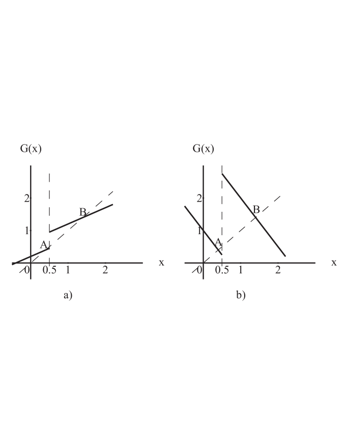
Figure 1: The map $x\mapsto G(x,\alpha,\gamma)$ for $\alpha=0.25$, $\gamma=-0.2$ (a) and $\alpha=1.25$, $\gamma=-1$ (b).

This equation is frequently used in biophysical problems, in the combustion theory, in chemical kinetics (e.g. in the theory of the Belousov–Zhabotinsky reaction), solid-state physics, etc. (see, for example, [23, 24, 25, 26]). One can see that the piecewise linear function $G(x,\alpha,\gamma)$ has a constant slope $(1-2\alpha)$. Depending on $\alpha$ the map $x\mapsto G(x,\alpha,\gamma)$ may exhibit qualitatively different behaviour. For $0<\alpha<1$ (see Fig.1a) it gives rise to a regular dynamics with one or two stable point, depending on the value of the parameter $\gamma$ (points A and B in Fig.1a), which are attractive for almost all points of the phase space. For $\alpha>1$ the slope of $G(x,\alpha,\gamma)$ is larger then one (see Fig.1b). That means, that for the finite motion of phase points the dynamics would be chaotic.

The uniform model (1) based on the coupled maps, which are described by functions (2), is known (see [22]). Following [22] consider this system as an $N$–dimensional piecewise–linear map $f:{\bf R}^{N}\to{\bf R}^{N}$. Because $G(x,\alpha,\gamma)$ is the piecewise–linear function with the constant derivative, the differential ${\rm D}_{f}$ of the map $f$ is a matrix with constant coefficients. This easily allows us to find the Lyapunov exponents $\lambda_{i}$ of such map. If $\rho_{s}$ are the eigenvalues of ${\rm D}_{f}$, then $\lambda_{s}=\ln|\rho_{s}|$. If among all the values $\rho_{s}$ there exists an eigenvalue located outside the unit circle on the complex plane, then any trajectory of the map $f$ is unstable. Otherwise the model has the regular dynamics. Thus, to know qualitatively the behavior of the system it is sufficient to find the location of the eigenvalues $\rho_{s}$ on the complex plane.

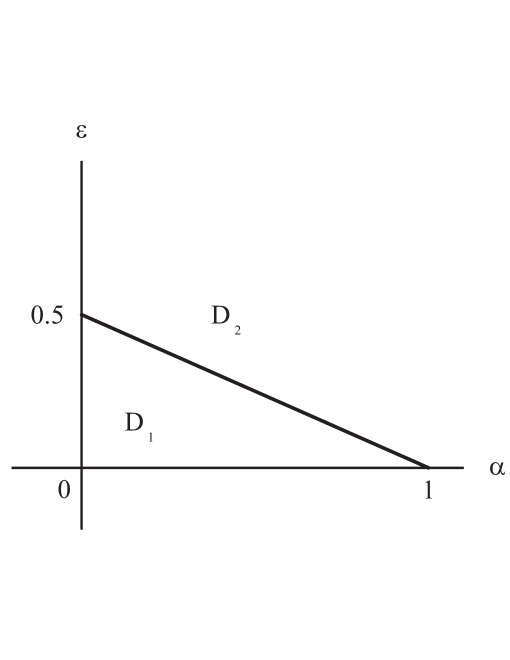
Figure 2: The parametric space of the homogeneous annular chain of the diffusively coupled maps (1), (2).

To find $\rho_{s}$ we should analyse the characteristic polynomial for the differential of the $N$–dimensional map, which may be expressed via the determinants of three–diagonal matrices of different dimension. For these determinants recurrent relations may be obtained. Taking the recurrent relations as difference equations with the given initial conditions we can find the solutions which are proportional to the Chebyshev polynomials with a linear function of the eigenvalues of ${\rm D}_{f}$ [22]. Using then the properties of the Chebyshev polynomials it can be shown that the characteristic polynomial may be reduced to the quadratic trinomial of a certain function $\rho_{s}$. Calculation of $\rho_{s}$ and analysis of their location on the complex plane shows that the parametric space of the system (1), (2) has two regions with qualitatively different behavior (Fig.2).

1. The region $D_{1}$, with the values of the parameters $\alpha$ and $\varepsilon$, which correspond to the regular dynamics of the model. This implies that the modules of all the eigenvalues of the differential of the map $f$ are less than unity.

2. The region $D_{2}$ where at least one of the eigenvalues $\rho_{s}$ satisfies the condition $|\rho_{s}|>1$. Generally, the system may have an infinite dynamics. However, if the dynamics is finite the system (1), (2) behaves chaotically [9, 10, 11].

The system (1), (2) is an uniform since all its elements are identical (one has the same map $x\mapsto G(x,\alpha,\gamma)$ for all the elements). Futher we will assume that each element of the system has the same map $x_{i}\mapsto G(x_{i},\alpha_{i},\gamma)$ but along the chain the values of the control parameter $\alpha_{i}$ may differ. We assume that only two types of elements exist in the system. The corresponding values we denote as $\alpha$ and $\beta$. As for the case of uniform system we will use the periodic boundary conditions, $x_{n+N}(k){\equiv}x_{n}(k)$.

2.2 The model with spatially periodic nonhomegeneity

The periodic spatial nonhomegeneity implies in our case that the chain has elements with alternating values of the parameters in the map $G$, e.g. $\alpha,\beta,\alpha,\beta,\ldots\$. This particular nonuniform model allows a complete analytical analysis.

Consider the system of coupled elements:

$$\cases{x_{n}(k+1)=G(x_{n}(k),\alpha,\gamma)+\varepsilon\Bigl{(}x_{n+1}(k)-2x_{n}(k)+x_{n-1}(k)\Bigr{)},&$n$ is odd,\cr\ &$\ $\cr x_{n}(k+1)=G(x_{n}(k),\beta,\gamma)+\varepsilon\Bigl{(}x_{n+1}(k)-2x_{n}(k)+x_{n-1}(k)\Bigr{)},&$n$ is even,\cr}$$ (3)

where $x_{n+N}(k)\equiv x_{n}(k)$, $N$ is even (to satisfy the periodic boundary condition), and the function $G$ is given by (2). To analyse the dynamics of this system we calculate the Lyapunov exponents using the approach described above.

The differential of the $N$–dimensional map corresponding to the system (3) reads

$${\rm D}_{f}\equiv Q_{N}=\left(\begin{array}[]{ccccc}1-2\varepsilon-2\alpha&\varepsilon&0&\ldots&\varepsilon\\ \varepsilon&1-2\varepsilon-2\beta&\varepsilon&\ldots&0\\ 0&\varepsilon&1-2\varepsilon-2\alpha&\ldots&0\\ \vdots&\vdots&\vdots&\ddots&\vdots\\ \varepsilon&0&0&\ldots&1-2\varepsilon-2\beta\end{array}\right)\ .$$

To find the eigenvalues $\rho_{s}$, $s=1,2,\ldots,N$ of the matrix $Q_{N}$, we calculate the determinant

$${\rm det}(Q_{N}-\rho I_{N})=\left|\begin{array}[]{cccccc}2z_{1}\varepsilon&\varepsilon&0&0&\ldots&\varepsilon\\ \varepsilon&2z_{2}\varepsilon&\varepsilon&0&\ldots&0\\ 0&\varepsilon&2z_{1}\varepsilon&\varepsilon&\ldots&0\\ \vdots&\vdots&\vdots&\vdots&\ddots&\vdots\\ 0&0&0&0&\ldots&\varepsilon\\ \varepsilon&0&0&0&\ldots&2z_{2}\varepsilon\end{array}\right|\ ,$$

with $z_{1}$ and $z_{2}$ defined by the relations $1-2\varepsilon-2\alpha-\rho=2z_{1}\varepsilon$, $1-2\varepsilon-2\beta-\rho=2z_{2}\varepsilon$. Making expansion of the determinant we obtain:

$${\rm det}(Q_{N}-\rho I_{N})=2z_{1}\varepsilon B_{N-1}-\varepsilon^{2}B_{N-2}-2\varepsilon^{N}-\varepsilon^{2}\hat{B}_{N-2},$$

where

$$B_{N}=\left|\begin{array}[]{ccccc}2z_{1}\varepsilon&\varepsilon&0&\ldots&0\\ \varepsilon&2z_{2}\varepsilon&\varepsilon&\ldots&0\\ 0&\varepsilon&2z_{1}\varepsilon&\ldots&0\\ \vdots&\vdots&\vdots&\ddots&\vdots\\ 0&0&0&\ldots&2z_{2}\varepsilon\end{array}\right|\ ,\ \ \ \ \hat{B}_{N}=\left|\begin{array}[]{ccccc}2z_{2}\varepsilon&\varepsilon&0&\ldots&0\\ \varepsilon&2z_{1}\varepsilon&\varepsilon&\ldots&0\\ 0&\varepsilon&2z_{2}\varepsilon&\ldots&0\\ \vdots&\vdots&\vdots&\ddots&\vdots\\ 0&0&0&\ldots&2z_{1}\varepsilon\end{array}\right|\ .$$

It is not hard to see that $\hat{B}_{N}(z_{1},z_{2})$ may be obtained from $B_{N}(z_{1},z_{2})$ exchanging the arguments $z_{1}\leftrightarrow z_{2}$. This suggest the way of finding $B_{N}(z_{1},z_{2})$ using the recurrent relation. Expanding $B_{N}$ (along the first line) we obtain:

$$\cases{B_{N}=2z_{1}\varepsilon B_{N-1}-\varepsilon^{2}B_{N-2},&$N$ is even;\cr\ &$\ $\cr B_{N}=2z_{2}\varepsilon B_{N-1}-\varepsilon^{2}B_{N-2},&$N$ is odd.}$$

This allows us to express determinants of the odd order via determinants of the even one,

$$B_{2N+1}=\frac{B_{2N+2}+\varepsilon^{2}B_{2N}}{2z_{1}\varepsilon}\ ,$$ (4)

and obtain then the recurrent relation for the even determinants

$$B_{2N}=\varepsilon^{2}(4z_{1}z_{2}-2)B_{2N-2}-\varepsilon^{4}B_{2N-4}\ .$$ (5)

One can treat Eq.(5) as a difference equation with the initial conditions

$$B_{0}=1,B_{2}=\varepsilon^{2}(4z_{1}z_{2}-1)\ .$$ (6)

Solving then (5), (6) together with (4), we arrive at:

$$\cases{B_{N}(z_{1},z_{2})=\varepsilon^{N}U_{N}(z),&for even $N$;\cr\ &$\ $\cr B_{N}(z_{1},z_{2})=\varepsilon^{N}\sqrt{\displaystyle\frac{z_{2}}{z_{1}}}U_{N}(z),&for odd $N$,\cr}$$

where $U_{N}(z)$ is the second order Chebyshev polynomial. In turn, for $\hat{B}_{N}(z_{1},z_{2})$ we get:

$$\cases{\hat{B}_{N}(z_{1},z_{2})=\varepsilon^{N}U_{N}(z),&for even $N$ ;\cr\ &$\ $\cr\hat{B}_{N}(z_{1},z_{2})=\varepsilon^{N}\sqrt{\displaystyle\frac{z_{1}}{z_{2}}}\ U_{N}(z),&for odd $N$.\cr}$$

Now, using the obtained relations for $B_{N-1}$, $B_{N-2}$ and $\hat{B}_{N-2}$, we finally arrive at:

$${\rm det}(Q_{N}-\rho I_{N})=2\varepsilon^{N}\Bigl{(}zU_{N-1}(z)-U_{N-2}(z)-1\Bigr{)}.$$ (7)

This allows us to find the eigenvalues of the differential of the map (3), (2). As follows from Eq.(7),

$$zU_{N-1}(z)-U_{N-2}(z)-1=0,$$ (8)

or, $T_{N}(z)-1=0$. Here we used the relation between the second order Chebyshev polynomials $U_{N}(z)$ and the first order $T_{N}(z)$. Since

$$T_{N}(z)=\frac{\left(z-\sqrt{z^{2}-1}\right)^{N}+\left(z-\sqrt{z^{2}-1}\right)^{-N}}{2},$$

where $z^{2}=z_{1}z_{2}$, then with $t=z-\sqrt{z^{2}-1}$ we obtain from Eq.(8):

$$\frac{1}{2}\left(t^{N}+\frac{1}{t^{N}}\right)-1=0$$

or $\displaystyle\left(t^{N}-1\right)^{2}=0$. Therefore, $t_{s}=e^{i\frac{2\pi}{N}s}$, $s=1,2,\ldots,N$, and $z_{s}=\cos(2\pi s/N),s=1,2,\ldots,N$. Taking into account that $2z_{1}\varepsilon\cdot 2z_{2}\varepsilon=4z^{2}\varepsilon^{2}$, we obtain a simple equation:

$$(1-2\varepsilon-2\alpha-\rho)(1-2\varepsilon-2\beta-\rho)=4\varepsilon^{2}\cos^{2}\left(\frac{2\pi}{N}s\right).$$

Solving it with respect to $\rho$, we find the set of eigenvalues of the differential of the map (3), (2):

$$\rho^{s}_{1,2}=1-2\varepsilon-\alpha-\beta\pm\sqrt{(\alpha-\beta)^{2}+4\varepsilon^{2}\cos^{2}\left(\frac{2\pi}{N}s\right)}\ ,$$ (9)

where $s=1,2,\ldots,N/2$. The dynamics of the system (3), (2) would be completely regular if all the values of $\rho_{s}$ were within the unit circle on the complex plane. Since all the $\rho^{s}_{1,2}$ are real, the condition of the regular dynamics is:

$$\cases{2\varepsilon+\alpha+\beta>\sqrt{4\varepsilon^{2}+(\alpha-\beta)^{2}},\cr\ \cr\displaystyle\varepsilon+\frac{\alpha+\beta}{2}+\sqrt{\varepsilon^{2}+\left(\frac{\alpha-\beta}{2}\right)^{2}}<1.\cr}$$

The first inequality is always realized when $\varepsilon,\alpha,\beta>0$. Thus, second one defines the restriction for the region with regular dynamics.

In its turn, in the region of the parametric space where the Lyapunov exponent $\lambda_{s}=\ln|\rho_{s}|>0$ the condition $\varepsilon+(\alpha+\beta)/2+\sqrt{\varepsilon^{2}+(\alpha-\beta)^{2}/4}>1$ is satisfied. Therefore, the boundary separating two regions with regular and chaotic dynamics is a surface in the three–dimensional parametric space $(\alpha,\beta,\varepsilon)$, which is given by the relation:

$$\varepsilon+\frac{\alpha+\beta}{2}+\sqrt{\varepsilon^{2}+\frac{(\alpha-\beta)^{2}}{4}}=1.$$ (10)

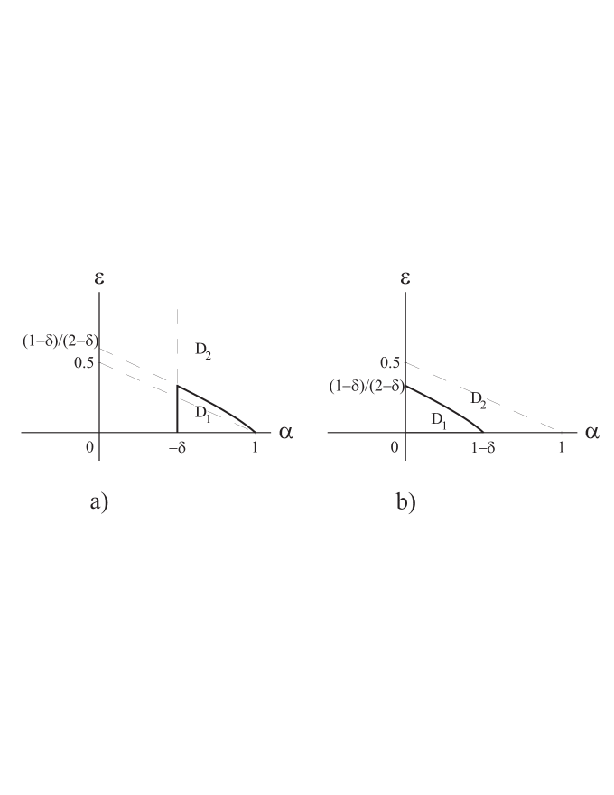
Figure 3: Cross–sections by the planes $\delta={\rm const}$ of the parametric space of the model (2), (3) for $-1<\delta<0$ (a) and $0<\delta<1$ (b).

To illustrate the obtained results we show in Fig.3 cross–sections of this surface by the planes $\delta={\rm const}$, with $\delta=\beta-\alpha$ being the nonhomegeneity parameter. Denote $D_{1}$ the region with regular dynamics and $D_{2}$ the region where $\lambda_{s}>0$. These two regions are separated by the boundary, defined (implicitly) by Eq.(10). In Fig.3 we also show by dashed line the corresponding boundary between $D_{1}$ and $D_{2}$ for the case of homogeneous $(\delta=0)$ system of coupled maps (Fig.2).

As it follows from the Fig.3, for $\delta>1$ for all values of $\varepsilon$, $\alpha$ the model demonstrates the chaotic dynamics. For $\delta<1$ the region $D_{1}$ arises where the system has regular dynamics. This region where $0<\delta<1$ is, in fact, a subregion of the corresponding region $D_{1}$ of the regular dynamics of the homogeneous model.

For $-1<\delta<0$ there exist such $\varepsilon$ and $\alpha$ that the homogeneous model exhibits the chaotic dynamics, while the inhomogeneous still has the regular one. Note that the restriction $\alpha>-\delta$ corresponds to the condition $\beta>0$. For $\delta<-1$ the region $D_{1}$ vanishes and for all $\varepsilon$, $\alpha$ the model (3), (2) demonstrates only the chaotic dynamics. As it also follows from Fig.3, two qualitatively different regimes make take place: $\alpha$ belongs to the region of the regular behavior, $\beta$ to the region of chaos with $\lambda_{s}>0$, with the global dynamics being regular. Similarly one can observe just the opposite case of the chaotic dynamics of the periodically inhomogeneous model. Realisation of the particular regime depends on the value of the diffusion constant $\varepsilon$.

2.3 Annular model with a single defect

Let us now turn to the case of spatially inhomogeneous model of diffusively coupled maps for the case of a single “defect”. In this case among $N$ element of the system only one element has the parameter $\beta$ (see (2)), while the other $(N-1)$ elements have parameter $\alpha$. Assume for simplicity that this element is located at $n=1$. Then we can write for this model:

$$\cases{x_{n}(k+1)=G(x_{n}(k),\alpha,\gamma)+\varepsilon\Bigl{(}x_{n-1}(k)-2x_{n}(k)+x_{n+1}(k)\Bigr{)},&$n=2,3,\ldots,N$,\cr\ \cr x_{1}(k+1)=G(x_{1}(k),\beta,\gamma)+\varepsilon\Bigl{(}x_{N}(k)-2x_{1}(k)+x_{2}(k)\Bigr{)},\cr}$$ (11)

where $x_{n+N}\equiv x_{n}(k),n=1,2,\ldots,N$. Let the function $G(x,\alpha,\gamma)$ is still given by (2). Calculate now the differential of the corresponding map for the system (11), (2):

$$D_{f}{\equiv}Q_{N}{=}\left(\begin{array}[]{ccccc}1-2\varepsilon-2\beta&\varepsilon&0&{\ldots}&\varepsilon\\ \varepsilon&1-2\varepsilon-2\alpha&\varepsilon&{\ldots}&0\\ 0&\varepsilon&1-2\varepsilon-2\alpha&{\ldots}&0\\ \vdots&\vdots&\vdots&{\ddots}&\vdots\\ \varepsilon&0&0&{\ldots}&1-2\varepsilon-2\alpha\\ \end{array}\right)\ .$$ (12)

If we apply the same approach as previously, to find the Lyapunov exponents of the model (11), (2), we should have to get the roots of the polynomial of the $2N+2$–th order. This can be done only numerically. Instead we will use somewhat different approach, which significantly facilitates the analysis.

Applying the estimate of the eigenvalues of the matrix (12) according to the Gershgorin’s theorem [27], we may evaluate the location of the region of the regular dynamics. By this theorem, all the eigenvalues of the matrix $A=\{a_{ij}\}_{n\times n}$ which belongs to the union of the discs on the complex plane:

$$\rho_{s}\in\bigcup\limits_{i=1}^{n}\Bigl{\{}z\in{\bf C}:|z-a_{ij}|\leq R^{\prime}_{i}\Bigr{\}}\ ,$$

where $s=1,2,\ldots,N$ and $R^{\prime}_{i}$ is either a row almost–norm of the matrix $A$, $R^{\prime}_{i}=\sum_{j=1\atop j\neq i}^{n}|a_{ij}|$, or a column almost–norm of the matrix $A$, $R^{\prime}_{j}=\sum_{i=1\atop i\neq j}^{n}|a_{ij}|$. Since the differential of the map (12) is a real symmetric matrix then, (i) the row and column almost–norms are equal, and (ii) the eigenvalues of the matrix ${\rm D}_{f}$ are real. Therefore, the Gershgorin’s discs transform on the real axis as:

$$\rho_{s}\in\bigcup\limits_{i=1}^{n}\Bigl{\{}z\in{\bf R}:|z-a_{ij}|\leq R^{\prime}_{i}\Bigr{\}},\ \ \ \ s=1,2,\ldots,N\ .$$

Because $\varepsilon>0$, from (12) we get:

$$R^{\prime}_{i}=\sum_{j=1\atop j\neq i}^{n}|a_{ij}|=|\varepsilon|+|\varepsilon|=2\varepsilon\ .$$

Moreover, since $R^{\prime}_{i}$ does not depend on $i$ and in the differential of map ${\rm D}_{f}$ (12) there exist only two different diagonal elements, the eigenvalues of ${\rm D}_{f}$ belong to the union of the two intervals:

$$\Bigl{\{}z\in{\bf R}:|1-2\varepsilon-2\alpha-z|\leq 2\varepsilon\Bigr{\}}\bigcup\Bigl{\{}z\in{\bf R}:|1-2\varepsilon-2\beta-z|\leq 2\varepsilon\Bigr{\}}.$$

Then, taking into account that $\alpha$, $\beta$, $\varepsilon>0$, we obtain the upper bound for the modules of the eigenvalues of ${\rm D}_{f}$:

$$|\rho_{s}|\leq\cases{\beta+2\varepsilon,&$\alpha<\beta$;\cr\ &$\ $\cr\alpha+2\varepsilon,&$\alpha>\beta$.\cr}$$

Thus, the region $\tilde{D}_{1}$ in the parametric space $(\alpha,\beta,\varepsilon)$, which satisfies the conditions

$$\tilde{D}_{1}:\qquad\cases{\beta+2\varepsilon<1,&if $\alpha<\beta$;\cr\ &$\ $\cr\alpha+2\varepsilon<1,&if $\alpha>\beta$;\cr}$$ (13)

corresponds to the regular dynamics of the inhomogeneous model (11), (2), while the region

$$\tilde{D}_{2}:\qquad\cases{\beta+2\varepsilon>1,&if $\alpha<\beta$;\cr&$\ $\cr\alpha+2\varepsilon>1,&if $\alpha>\beta$;\cr}$$ (14)

corresponds to the positive $\lambda_{s}$.

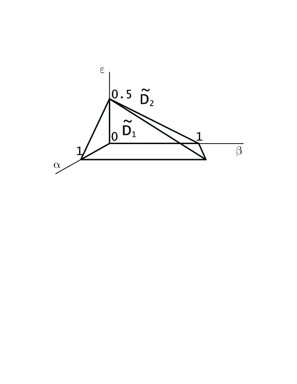
Figure 4: The estimate of the region with the regular dynamics for the inhomogeneous chains with two types of elements in the parametric space $(\alpha,\beta,\varepsilon)$.

The regions $\tilde{D}_{1}$ and $\tilde{D}_{2}$ are shown in Fig.4. The region $\tilde{D}_{1}$ is the lower bound of the region with the regular dynamics, because it is obtained via the upper bound of the eigenvalues of the map differential. This means that any point of $\tilde{D}_{1}$ would correspond to the regular dynamics, while any point of $\tilde{D}_{2}$ would correspond either the regular dynamics, or (if the motion is finite) the chaotic one.

It is significant that the obtained estimate is applicable not only for the model with a single defect, but for a wide class of annular chains of maps with diffusive coupling (1), which have only two types of elements $\Big{(}$with different parameters $\alpha_{i}$ in the function $G(x_{i},\alpha_{i},\gamma)\Big{)}$. This follows from the fact that the particular number of elements of each type and their mutual location is not important. Indeed, almost–norms of the differentials of the maps of all such systems are the same and the centres of the two possible intervals, which contain according to the Gershgorin’s theorem, the eigenvalues of ${\rm D}_{f}$, do coincide.

In the case when the two intervals, which we use to estimate $\rho_{s}$, do not intersect, there is, according to the Gershgorin’s theorem, “clusterization” of the eigenvalues of the differential of the map. Namely, $q$ eigenvalues $\rho_{s}$, $s=1,2,\ldots,q$, will belong to one interval, and $(N-q)$ eigenvalues $\rho_{s}$, $s=q+1,q+2,\ldots,N$ will belong to the other interval. Here $q$ is the number of elements with parameter $\alpha$, and, respectively, $(N-q)$ is the number of elements with parameter $\beta$. Unfortunately, this does not help to improve the estimate of the region with the regular dynamics.

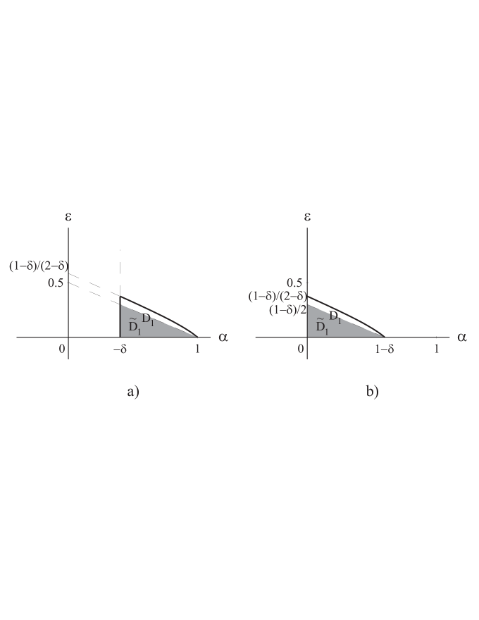
Figure 5: The estimate and the exact result for the region with the regular dynamics for the model with periodic nonhomegeneity for $-1<\delta<0$ (a) and $0<\delta<1$ (b).

Let us compare the estimate (13) with the exact result, that has been obtained above for the model with the periodic nonhomegeneity. Obviously, the latter model belongs to the class of models for which the this estimate holds true. To illustrate this we show the cross–sections $\delta={\rm const}$ of the region $D_{1}$, which corresponds to the regular dynamics of (3), (2), and of its estimate, the region $\tilde{D}_{1}$ (see Fig.5). From Fig.5 it follows that the estimate (13) of the region with the regular dynamics is rather adequate, however it does not show that for $-1<\delta<0$ the region of the regular dynamics of (3), (2) includes the region of the regular dynamics of the spatially homogeneous system.

Turn now to the map (11), (2), which refer to the case of a single defect and find the eigenvalues of the differential of map (12) numerically. One can write for the characteristic polynomial:

$${\rm det}(Q_{N}-\rho I_{N})=\left|\begin{array}[]{ccccc}2z\varepsilon+2(\alpha-\beta)&\varepsilon&0&\ldots&\varepsilon\\ \varepsilon&2z\varepsilon&\varepsilon&\ldots&0\\ 0&\varepsilon&2z\varepsilon&\ldots&0\\ \vdots&\vdots&\vdots&\ddots&\vdots\\ \varepsilon&0&0&\ldots&2z\varepsilon\end{array}\right|,$$

where $2z\varepsilon=1-2\varepsilon-2\alpha-\rho$. Expanding ${\rm det}(Q_{N}-\rho I_{N})$ in the first line we arrive at

$${\rm det}(Q_{N}-\rho I_{N})=[2z\varepsilon+2(\alpha-\beta)]B_{N-1}-2\varepsilon^{2}B_{N-2}-2(-1)^{N}\varepsilon^{N},$$ (15)

with

$$B_{N}=\left|\begin{array}[]{ccccc}2z\varepsilon&\varepsilon&0&\ldots&0\\ \varepsilon&2z\varepsilon&\varepsilon&\ldots&0\\ 0&\varepsilon&2z\varepsilon&\ldots&0\\ \vdots&\vdots&\vdots&\ddots&\vdots\\ 0&0&0&\ldots&2z\varepsilon\end{array}\right|.$$

As previously, we use the first line factorization of $B_{N}$ to obtain the recurrent relation, $B_{N}=2z\varepsilon B_{N-1}-\varepsilon^{2}B_{N-2}$. Using the initial conditions, $B_{1}=2z\varepsilon$, $B_{2}=\varepsilon^{2}(4z^{2}-1)$, we obtain:

$$B_{N}=\varepsilon^{N}U_{N}(z),$$ (16)

where $U_{N}(z)$ is the second order Chebyshev polynomial. Taking into account Eq.(16) and representation of $U_{N}(z)$,

$$U_{N}(z)=\frac{(z+\sqrt{z^{2}-1})^{N+1}-(z-\sqrt{z^{2}-1})^{N+1}}{2\sqrt{z^{2}-1}}=\frac{\left(\displaystyle\frac{1}{t}\right)^{N+1}-t^{N+1}}{\displaystyle\frac{1}{t}-t}\ ,$$

where $t=z-\sqrt{z^{2}-1}$, we recast Eq.(15) into the following form:

$${\rm det}(Q_{N}-\rho I_{N})=2\varepsilon^{N}\left[\frac{t^{2N+1}+1}{2t^{N}}+\left(\frac{\alpha-\beta}{\varepsilon}\right)\frac{1-t^{2N}}{(1-t^{2})t^{N-1}}-(-1)^{N}\right].$$

Thus, the characteristic equation for the differential of the map (12) reads

$$t^{2N+2}+2\left(\displaystyle\frac{\alpha-\beta}{\varepsilon}\right)t^{2N+1}-t^{2N}-2(-1)^{N}t^{N+2}+2(-1)^{N}t^{N}+t^{2}-2\left(\displaystyle\frac{\alpha-\beta}{\varepsilon}\right)t-1=0.$$

Finding numerically the roots of this equation, we obtain $\rho_{s}$. Comparing $\rho_{s}$ with unity for different sets of $\alpha$, $\beta$, $\varepsilon$, for the annular chain of diffusively coupled maps with a single defect we find the regions $D_{1}$ and $D_{2}$ with qualitatively different dynamics. In Fig.6 we show cross–sections of these regions by the planes with the fixed values of $\delta={\rm const}$, where $\delta=\beta-\alpha$. The estimate (13) of the region with the regular dynamics is marked by the dashed line. As in the case of the periodic nonhomegeneity, the actual region for positive $\delta$ is larger than that predicted by the estimate. However for the negative $\delta$ the estimate is in a perfect agreement with the numerical results as well as with the results corresponding to the homogeneous chain. Thus, if one of the elements of the chain had the parameter smaller than that of the others, there would be no impact on the global dynamics of the system. On the other hand, if the parameter which refers to the defect had larger value than that of the other elements, this would diminish the region of the regular dynamics as compared to the case of the uniform system.

3 Conclusions

We investigated the dynamics of diffusively coupled one–dimensional maps, which model one–dimensional excitable medium with space nonhomegeneity. We considered different types of the nonhomogeneities. For all systems, with the spatial nonhomegeneity, which may be described in terms of two types of elements with different values of the control parameter, we found analytically a lower bound of the region in the parametric space where the ensemble exhibits the regular dynamics. This estimate has been obtained by localizing the eigenvalues of the differential of the map. For two different model of this class we also obtained exact analytical and numerical results which completely characterize the dynamics of the system.

We observed that all three approaches (the approximate analytical analysis of the chain with two types of elements (13), the exact solution for the spatially periodic defects (§2.2) and numerical study (§2.3) of the model with a single defect) show the possibility of two qualitatively different types of the ensemble behavior. In the first case the system demonstrates a regular global behavior when one value of its parameter belongs to the region with the regular dynamics and the other one belongs to the region with the unstable dynamics. Vice versa, in the second case the global dynamics occurs to be unstable, and if the motion is finite — chaotic. The particular type of the chain behavior depends on the diffusive parameter $\varepsilon$. Obviously, if $\varepsilon$ is large enough, the global dynamics would not be regular.

We wish to stress that according to our knowledge, the present study is the first attempt of the analytical description of the dynamics of inhomogeneous systems of coupled maps. These systems, being of significant importance from the point of view of applications, may exhibit a rich physical behavior, giving rise to a lot of new and interesting problems. One can mention such problems as properties of the wave travelling along the chain and influence of the defects on these motions, dynamics of the ensemble with time–dependent parameters, controllability conditions, synchronization and many others (see, e.g., [29, 30, 31, 18, 19, 20]). These problems, not discussed here will be addressed elsewhere [28, 32].

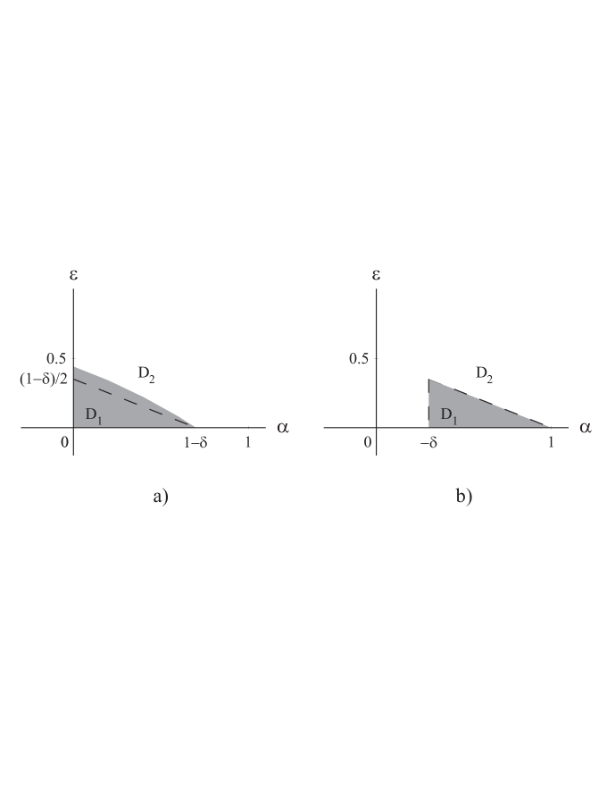
Figure 6: Cross–sections by the planes $\delta={\rm const}$ of the parametric space for the chain of $N=20$ elements with a single defect for $\delta=-0.3$ (a) and $\delta=0.3$ (b).

References

- [1] K.Kaneko. Pattern dynamics in spatio-temporal chaos.— Physica D, 1989, v.34, p.1–41.
- [2] K.Kaneko. Spatiotemporal chaos in one– and two–dimensional coupled map lattices.— Physica D, 1989, v.37, p.60–82.
- [3] L.A.Bunimovich, Ya.G.Sinai. Statistical mechanics of coupled map lattices.— In: Theory and Applications of Coupled Map Lattices, ed. K.Kaneko.— Wiley, 1993, p.169–189.
- [4] A.S.Mikhailov, A.Loskutov. Chaos and Noise.— Springer, Berlin, 1996.
- [5] M.Bär, M.Eiswirth. Turbulence due to spiral break–up in continuous excitable medium.— Phys. Rev. E, 1993, v.48, p.1635–1637.
- [6] Zhilin Qu, J.N.Weiss, A.Garfinkel. Spatiotemporal chaos in a simulated ring of cardiac cells.— Phys. Rev. Lett., 1997, v.58, p.1378–1390.
- [7] S.Morita. Lyapunov analysis of collective behaviour in a network of chaotic elements.— Phys. Lett. A, 1997, v.226, p.172–178.
- [8] A.P.Muñuzuri, V.Perez-Muñuzuri, M.Gomez-Gesteira, L.O.Chua, V.Perez-Villar. Spatio–temporal structures in discretely-coupled arrays of nonlinear circuits: a review.— Int. J. Bif. and Chaos, 1995, v.5, p.17–50
- [9] L.A.Bunimovich. Coupled map lattices: one step forward and two steps back.— Physica D, 1995, v.86, p.248–255.
- [10] Theory and Applications of Coupled Map Lattices, ed. K.Kaneko.— Wiley, 1993.
- [11] Chaos Focus Issue on Coupled Map Lattices.– Chaos, 1992, v.2, No3.
- [12] K.Kaneko. Clustering, coding, switching, hierarchical ordering, and control in a network of chaotic elements.— Physica D, 1990, v.41, p.137–172.
- [13] L.A.Bunimovich, Ya.G.Sinai. Space-time chaos in coupled map lattices.— Nonlinearity, 1988, v.1, p.491–504.
- [14] L.A.Bunimovich, S.Venkatagiri. On one mechanism of transition to chaos in lattice dynamical systems.— Phys. Rep., 1997, v.290, p.81–100.
- [15] G.Perez, S.Sinha, H.Cerdeira. Nonsimultaneity effects in globally coupled maps.— Phys. Rev. E, 1996, v.54, p.6936–6939.
- [16] W.Just. Bifurcations in globally coupled map lattices.— J. Stat. Phys., 1995, v.79, p.429–449.
- [17] K.Kaneko. Globally coupled circle maps.— Physica D, 1991, v.54, p.5–19.
- [18] KaiEn Zhu, T.Chen. Controlling spatiotemporal chaos in coupled map lattices.— Phys.Rev.E, 2001, v.63, 067201, 1–4.
- [19] B.Hu, Z. Liu. Phase synchronization of two-dimensional lattices of coupled chaotic maps.— Phys.Rev.E, 2000, v.62, p.2114–2118.
- [20] M.Mehta, S.Sinha. Asynchronous updating of coupled maps leads to synchronization.— Chaos, 2000, v.10, p.350–358.
- [21] A.Sharma, N.Gupte. Spatiotemporal intermittency and scaling laws in inhomogeneous coupled map lattices.— Phys. Rev.E, 2002, v.66, No3, Art. No. 036210 Part 2A.
- [22] V.S.Afraimovich, V.I.Nekorkin, G.V.Osipov, and V.D.Shalfeev. Stability, Patterns and Chaos in Nonlinear Synchronised Lattices.— Inst. Appl. Phys. Press, Gorky, 1989 (Russian).
- [23] V.A.Vasiliev, Yu.M.Romanovsky, and V.G.Yakhno. Autowave Processes.— Nauka, Moscow, 1987.
- [24] Autowave Processes in Systems with Diffusion.— Inst. Appl. Phys. Press, Gorky, 1981 (Russian).
- [25] Ya.B.Zeldovich, G.I.Barenblatt, V.B.Librovich.. Mathematical Theory of Combustion and Explosion.— Moscow, Nauka, 1980 (Russian).
- [26] D.G.Aronson, H.F.Weinberger. Nonlinear diffusion in population genetics, combustion and nerve pulse propagation.– Lect. Notes in Math., 1975, v.446, p.5–49.
- [27] R.A. Horn and C.R. Johnson. Matrix Analysis.— Cambridge University Press, USA, 1985.
- [28] A.Loskutov, A.K.Prokhorov and S.D.Rybalko. Analysis of inhomogeneous chains of coupled quadratic maps.— Theor. and Math. Physics, 2002, v.132, No1, p.980–996.
- [29] N.Parekh, S.Sinha. Controllability of spatiotemporal systems using constant pinnings.— Physica A, 2003, v.318 No1–2, p.200-212.
- [30] S.H.Wang, J.H.Xiao, et al. Spatial orders appearing at instabilities of synchronous chaos of spatiotemporal systems.— European Phys. J., 2002, v.30, No4, p.571–575.
- [31] C.A.C.Jousseph, S.E.D.Pinto, L.C.Martins, M.W.I.Beims. Influence of impurities on the dynamics and synchronization of coupled map lattices.— Physica A, 2003, v.317, No3–4, p.401–410.
- [32] A.Loskutov, S.D.Rybalko, R.Seleznev.— To be published.