Semiclassical form factor for spectral and matrix element fluctuations of multidimensional chaotic systems

Abstract

We present a semiclassical calculation of the generalized form factor $K_{ab}(\tau)$ which characterizes the fluctuations of matrix elements of the operators $\hat{a}$ and $\hat{b}$ in the eigenbasis of the Hamiltonian of a chaotic system. Our approach is based on some recently developed techniques for the spectral form factor of systems with hyperbolic and ergodic underlying classical dynamics and $f=2$ degrees of freedom, that allow us to go beyond the diagonal approximation. First we extend these techniques to systems with $f>2$. Then we use these results to calculate $K_{ab}(\tau)$. We show that the dependence on the rescaled time $\tau$ (time in units of the Heisenberg time) is universal for both the spectral and the generalized form factor. Furthermore, we derive a relation between $K_{ab}(\tau)$ and the classical time–correlation function of the Weyl symbols of $\hat{a}$ and $\hat{b}$.

I Introduction

I.1 Overview

In a number of recent works the quantum spectral statistics of closed chaotic systems was investigated in the semiclassical limit. According to a conjecture by Bohigas, Giannoni and Schmit BGS84 (BGS), the fluctuations of the energy levels are system–independent and coincide with the predictions of random–matrix theory (RMT) if the system has a chaotic underlying classical dynamics. Numerical and experimental investigations carried out on a great variety of systems support the BGS conjecture Haake ; Stoeckmann .

In the semiclassical limit, Gutzwiller’s trace formula Gutzwiller90 provides a suitable starting point for the calculation of spectral correlation functions. It relates the quantum mechanical density of states to a sum over classical periodic orbits which are characterized by an amplitude and a phase that is obtained from the action of the orbit. A prominent example of a quantum correlation function is the two–point energy–energy correlation function and its Fourier transform, the spectral form factor $K(\tau)$. In this case a semiclassical analysis faces the problem of evaluating a double sum over periodic orbits which requires an appropriate quantitative treatment of classical action correlations. Averaging the form factor of a given system over an energy window that is large compared to the mean level spacing implies that only pairs of orbits with a small action difference of the order of $\hbar$ yield significant contributions. The leading contribution given by the terms with vanishing action difference is obtained within the diagonal approximation Berry85 . This approximation accounts for all orbit pairs where an orbit is associated to itself or to its time–reversed partner if time–reversal symmetry is present.

Only recently a method for a systematic inclusion of certain orbit pairs with small but nonzero action differences was developed for systems with time–reversal symmetry Sieber01 ; Sieber02 . This approach, originally formulated in the configuration space, was first applied to the next-to-leading order correction of the spectral form factor of a uniformly hyperbolic system showing agreement with the RMT predictions. In subsequent works, extensions to a phase–space formulation applicable to nonuniformly hyperbolic systems Spehner03 ; Turek03 and to higher–order corrections Mueller04 were proposed. However, all these previous considerations were restricted to systems with $f=2$ degrees of freedom, e.g., two–dimensional billiards, while the more general RMT conjecture is independent of $f$. In this work, we present a theory which applies to hyperbolic and ergodic Hamiltonian systems with an arbitrary number $f$ of degrees of freedom ($f\geq 2$). These systems are characterized by a set of system–specific time scales, namely the $(f-1)$ positive Lyapunov exponents. However, we will prove that going beyond the diagonal approximation the final result for the spectral form factor is independent of $f$ and coincides in a universal way with the RMT predictions.

From an experimental point of view it is desirable to furthermore develop a theory that describes not only statistical properties of the energy spectrum but also of quantum mechanical matrix elements, as entering, for example, in cross sections. The fluctuations of the diagonal matrix elements of the operators $\hat{a}$ and $\hat{b}$ in the eigenbasis of the Hamiltonian can be described by a generalized form factor Eckhardt95 $K_{ab}(\tau)$.

Similarly to the spectral form factor, one expects that $K_{ab}(\tau)$ also shows universal features as $\hbar\to 0$ and depends only on averaged classical quantities, like the averages over the constant–energy surface and the time correlation function of the Weyl symbols of $\hat{a}$ and $\hat{b}$. Analytical results exclusively based on the diagonal approximation have to some extent confirmed this statement Eckhardt95 ; EFKAMM95 ; Eckhardt97 ; Eckhardt00 . In this work, we generalize these results beyond the diagonal approximation.

In the following two subsections we briefly recall the semiclassical theory for the form factor based on Gutzwiller’s trace formula. In section II, we discuss the diagonal approximation and the origin of the off–diagonal corrections in the special case of the spectral form factor. We then show how the results for two–dimensional systems can be extended to higher–dimensional ones, leading once more to universality and agreement with RMT predictions in the semiclassical limit. The matrix–element fluctuations described by the generalized form factor $K_{ab}(T)$ are then studied in Section III. The leading–order (diagonal approximation) and next-to-leading-order terms are determined.

I.2 Generalized form factor: definitions and main results

We introduce the weighted density of states

$$d_{a}(E)\equiv{\rm tr}\left(\hat{a}\,\delta(E-\hat{H})\right)=\sum\limits_{n}\langle n|\hat{a}|n\rangle\,\delta(E-E_{n})\,$$ (1)

for a quantum observable $\hat{a}$. This is in generalization of the spectral density of states where $\hat{a}$ is given by the identity operator, i.e., $\hat{a}=\hat{1}$. In Eq. (1), $|n\rangle$ are the eigenstates and $E_{n}$ the corresponding eigenenergies of the Hamiltonian $\hat{H}$ of the system. The two–point correlation function

$$R_{ab}(\epsilon)\equiv\frac{1}{\left\langle d(E)\right\rangle_{\Delta E}^{2}}\left(\left\langle d_{a}\left(E-\frac{\epsilon}{2}\right)d_{b}\left(E+\frac{\epsilon}{2}\right)\right\rangle_{\Delta E}-\biggl{\langle}d_{a}(E)\biggr{\rangle}_{\Delta E}\biggl{\langle}d_{b}(E)\biggr{\rangle}_{\Delta E}\right)$$ (2)

describes correlations between the diagonal matrix elements of $\hat{a}$ and $\hat{b}$ in the eigenbasis $\{|n\rangle\}$. In Eq. (2), $\left\langle d(E)\right\rangle_{\Delta E}$ is the mean density of states, given by $\left\langle d(E)\right\rangle_{\Delta E}=\Omega/(2\pi\hbar)^{f}$, where $f$ is the number of degrees of freedom of the system and $\Omega=\int{\rm d}{\bf x}\,\delta(E-H({\bf x}))$ the volume of the constant–energy surface in phase space. The brackets $\langle\dots\rangle_{\Delta E}$ denote a smooth (e.g., Gaussian) energy average over an energy window $\Delta E$ much larger than the mean level spacing but classically small, i.e., $\langle d(E)\rangle_{\Delta E}^{-1}\ll\Delta E\ll E$. The mean density of states determines the Heisenberg time,

$$T_{H}\equiv 2\pi\hbar\left\langle d(E)\right\rangle_{\Delta E}\,.$$ (3)

As shown in Ref. Prange97 , a second average is required to obtain a self–averaging quantity for the Fourier transform of the correlation function $R_{ab}(\epsilon)$. We thus introduce the form factor as a time average of the Fourier transform of $R_{ab}(\epsilon)$ over a time window $\Delta T$, with $\Delta T\ll T_{H}$ (for instance, $\Delta T=2\pi\hbar/\Delta E)$. Denoting by $h(\epsilon)$ the Fourier transform of the weight function in the time average, we define

$$K_{ab}(T)\equiv\langle d(E)\rangle_{\Delta E}\int\limits_{-\infty}^{\infty}{\rm d}\epsilon\,e^{-i\epsilon T/\hbar}\,h(\epsilon)\,R_{ab}(\epsilon)\,.$$ (4)

This generalized form factor which has been introduced in Ref. Eckhardt95 will be the central quantity of this paper. For definiteness, we consider a uniform average over a time window $[T-\Delta T/2,T+\Delta T/2]$ implying $h(\epsilon)=(\epsilon\Delta T/2\hbar)^{-1}\sin(\epsilon\Delta T/2\hbar)$.

Setting $\hat{a}=\hat{b}=\hat{1}$ in Eqs. (2) and (4), one recovers the well–known spectral form factor $K(T)\equiv K_{11}(T)$. The correlation function $R(\epsilon)$ and its Fourier transform (4) have been calculated based on random–matrix assumptions. For systems with time–reversal symmetry, the relevant random–matrix ensemble is the Gaussian orthogonal ensemble (GOE) and yields the spectral form factor

$$K^{\text{}}(\tau) = 2\tau-\tau\ln(1+2\tau)\;\;\;,\;\;\;0<\tau<1$$ (5)

$$= 2\tau-2\tau^{2}+{\mathcal{O}}(\tau^{3})\;,$$

independent of the dimensionality $f$ of the system. Here, $K(\tau)$ is expressed in terms of the rescaled time $\tau=T/T_{H}$.

As follows from Snirelman’s theorem Snirelman74 , the corresponding generalized form factor reads, to leading order in $\hbar$,

$$K_{ab}(\tau)\simeq\overline{a({\bf x})}\;\overline{b({\bf x})}\,K(\tau)$$ (6)

(see section III below). Here, the average $\overline{a({\bf x})}$ of the Weyl symbol $a({\bf x})$ of the quantum observable $\hat{a}$ is taken with respect to the Liouville measure,

$$\overline{a({\bf x})}\equiv\frac{1}{\Omega}\int{\rm d}{\bf x}\,\delta(E-H({\bf x}))\,a({\bf x})\,,$$ (7)

see also (10). The phase–space coordinates are denoted by ${\bf x}=({\bf q},{\bf p})$. In many interesting situations $\overline{a({\bf x})}=\overline{b({\bf x})}=0$ which can always be obtained by shifting $a({\bf x})\to a({\bf x})-\overline{a({\bf x})}$. This implies, according to Eq. (6), a vanishing $K_{ab}(\tau)$ for $\hbar\to 0$. In this case, our semiclassical methods will enable us to go beyond the result (6). We will show that the correction terms to Eq. (6) are of order $1/T_{H}\sim\hbar^{f-1}$ and given by

$$K_{ab}\left(\tau\right)\approx\frac{1}{\tau T_{H}}\,\left[2\tau-2\tau^{2}+{\cal O}(\tau^{3})\right]\,\int\limits_{0}^{\infty}{\rm d}t\,C^{S}_{ab}(t)\;.$$ (8)

Here the classical time–correlation function $C^{S}_{ab}(t)$ is defined as

$$C^{S}_{ab}(t)\equiv\overline{a({\bf x})b^{S}({\bf x}_{t})}\quad\text{with}\quad b^{S}({\bf x})=\frac{b({\bf x})+b({\cal T}{\bf x})}{2}\;,$$ (9)

where $\overline{a({\bf x})}=\overline{b({\bf x})}=0$ is implicitly used, ${\mathcal{T}}:({\bf q},{\bf p})\mapsto({\bf q},-{\bf p})$ is the time–reversal map, and ${\bf x}_{t}$ is the solution of the classical equations of motion with initial condition ${\bf x}_{0}={\bf x}$. The symmetrized form $b^{S}({\bf x})$ of $b({\bf x})$ enters as the dynamics is assumed to be invariant with respect to time reversal.

I.3 Semiclassical limit

In the semiclassical approach, the Weyl symbol of the operator $\hat{a}$,

$$a({\bf q},{\bf p})\equiv\int{\rm{d}}{\bf q}^{\prime}\,e^{{\rm{i}}\,{\bf p}\cdot{\bf q}^{\prime}/\hbar}\,\Bigl{\langle}{\bf q}-\frac{{\bf q}^{\prime}}{2}\Bigl{|}\,\hat{a}\,\Bigr{|}{\bf q}+\frac{{\bf q}^{\prime}}{2}\Bigr{\rangle}$$ (10)

plays an important role (see, e.g., Ref. Balazs84 ). It is a function of the phase–space coordinates ${\bf x}=({\bf q},{\bf p})$ and tends in the limit $\hbar\to 0$ to the corresponding classical observable. In the following we assume that $a({\bf x})$ is a smooth function of ${\bf x}$. The semiclassical evaluation of Eq. (1) for classically chaotic quantum systems yields the generalized Gutzwiller trace formula Eckhardt92 ; Combescure99

$$d_{a}(E)=\left\langle d_{a}(E)\right\rangle_{\Delta E}+d_{a}^{\rm osc}(E)\;,$$ (11)

with

$$\left\langle d_{a}(E)\right\rangle_{\Delta E}=\frac{\Omega}{(2\pi\hbar)^{f}}\;\overline{a({\bf x})}$$ (12)

and

$$d^{\rm osc}_{a}(E)=\frac{1}{\pi\hbar}{\rm Re}\left\{\sum_{\gamma}{\cal A}_{\gamma}\exp\left({\rm i}\frac{S_{\gamma}}{\hbar}\right)\right\}.$$ (13)

The mean weighted density of states, $\left\langle d_{a}(E)\right\rangle_{\Delta E}$, depends on the dimensionality $f$ of the system and is determined by the average (7) of $a({\bf x})$ over the constant–energy surface. The oscillatory contribution, Eq. (13), is given by a sum over classical periodic orbits labeled by $\gamma$. The weights ${\cal A}_{\gamma}$ are related to the amplitudes Gutzwiller90

$$w_{\gamma}=\frac{(T_{\gamma}/r_{\gamma})\exp(-{\rm i}\pi\mu_{\gamma}/2)}{\sqrt{|\det(M_{\gamma}-1)|}}$$ (14)

via the relation ${\cal A}_{\gamma}=w_{\gamma}A_{\gamma}$, where $T_{\gamma}$ is the period of the orbit $\gamma$, $r_{\gamma}$ its repetition number, $\mu_{\gamma}$ its Maslov index, $M_{\gamma}$ its stability matrix, and

$$A_{\gamma}=A({\bf x}_{0}^{\gamma},T_{\gamma})\equiv\frac{1}{T_{\gamma}}\int\limits_{0}^{T_{\gamma}}\,{\rm d}t\,a({\bf x}_{t}^{\gamma})\;.$$ (15)

Here, ${\bf x}_{t}^{\gamma}$ is the phase–space point on the periodic orbit $\gamma$ obtained by solving the classical equations of motion with the initial condition ${\bf x}_{0}$, so that ${\bf x}^{\gamma}_{t+T_{\gamma}}={\bf x}^{\gamma}_{t}$. The applicability of the semiclassical expression (13) to chaotic systems with more than two degrees of freedom has been extensively studied in Ref. Primack00 .

Only the oscillating parts of $d_{a}(E)$ and $d_{b}(E)$ contribute to the correlation function (2). Substituting Eq. (13) into Eq. (4), one obtains

$$K_{ab}(T)=\frac{1}{T_{H}}\left\langle\sum\limits_{\gamma,\bar{\gamma}}{\cal A}_{\gamma}{\cal B}_{\bar{\gamma}}^{*}\;\exp\left({\rm i}\frac{S_{\gamma}-S_{\bar{\gamma}}}{\hbar}\right)\;\delta_{\Delta T}\left(T-\frac{T_{\gamma}+T_{\bar{\gamma}}}{2}\right)\right\rangle_{\Delta E}$$ (16)

by generalizing the corresponding steps of the semiclassical derivation of the spectral form factor Haake . In Eq. (16), the delta function with a finite width, $\delta_{\Delta T}(T^{\prime})$, originates from our choice of time averaging in Eq. (4). It is equal to $\Delta T^{-1}$ if $-\Delta T/2\leq T^{\prime}\leq\Delta T/2$ and zero otherwise. The semiclassical formula (16) of $K_{ab}(T)$ is the starting point of a further semiclassical evaluation. It contains a double sum over terms which strongly fluctuate with energy and poses the challenge to approximately compute its energy average.

An earlier approach to this problem is presented in Ref. Bogomolny96 where the correlation function (2) is considered directly instead of the form factor. It was shown that the off–diagonal contributions can be related to the diagonal terms yielding the leading order oscillatory term of the corresponding RMT result of $R(\epsilon)$ for large $\epsilon$. Furthermore, it was pointed out that in the case of a weighted density of states these contributions vanish to leading semiclassical order if the microcanonical average of the corresponding observable is zero. In this work we proceed in a different way and restrict our considerations to the form factor in the limit of small $\tau=T/T_{H}\ll 1$, see Subsection III.1 for our corresponding results concerning the weighted density of states.

In the following section we first discuss the case of the spectral form factor and then generalize our approach to include matrix element fluctuations in Section III.

II Spectral form factor for $f$-dimensional systems

II.1 Semiclassical evaluation within the diagonal approximation

A semiclassical expression for the spectral form factor $K(\tau)=K_{11}(\tau)$ is given by Eq. (16) with ${\cal A}_{\gamma}=w_{\gamma}$, ${\cal B}_{\bar{\gamma}}=w_{\bar{\gamma}}$ and the rescaled time $\tau=T/T_{H}$. To leading order in $\hbar$ and $\tau$, the double sum over periodic orbits can be evaluated by means of the so–called diagonal approximation Berry85 . It is guided by the fact that the contributions from pairs $(\gamma,\overline{\gamma})$ of orbits with action differences larger than $\hbar$ strongly fluctuate in energy and are therefore suppressed upon energy averaging. Hence the main contribution stems from the pairs of orbits with equal actions $S_{\gamma}=S_{\bar{\gamma}}$. If the system has no other than time–reversal symmetry then these pairs are obtained (up to accidental action degeneracies) by pairing each orbit $\gamma$ with itself or with its time–reversed version $\gamma^{i}$. To calculate the corresponding contribution to the semiclassical form factor (16), one has to perform a weighted periodic–orbit average of the type

$$\left\langle\dots\right\rangle_{{\rm po},T}\equiv\frac{1}{T}\sum\limits_{\gamma}\dots|w_{\gamma}|^{2}\delta_{\Delta T}(T-T_{\gamma}).$$ (17)

This is achieved by means of the following sum rule for periodic orbits in chaotic systems Parry90 :

$$\left\langle\frac{1}{T_{\gamma}}\int\limits_{0}^{T_{\gamma}}{\rm d}t\,f({\bf x}_{t}^{\gamma})\right\rangle_{{\rm po},T}\simeq\frac{1}{T}\int\limits_{0}^{T}{\rm d}t\,f({\bf x}_{t})\simeq\overline{f({\bf x})}$$ (18)

with $T\to\infty$. On the left–hand side the arbitrary continuous function $f({\bf x})$ is integrated along the periodic orbits $\gamma$ with periods $T_{\gamma}$ lying in the interval $[T-\Delta T/2,T+\Delta T/2]$. The integral on the right–hand side of Eq. (18) is taken along a nonperiodic “ergodic” trajectory which uniformly and densely fills the constant–energy surface. For ergodic systems this time average is equal to the phase–space average $\overline{f({\bf x})}$ in the large $T$ limit. In the special case $f({\bf x})=1$, Eq. (18) is known as the Hannay-Ozorio de Almeida sum rule HODA84 .

For a fixed rescaled time $\tau=T/T_{H}$, the periods $T_{\gamma}$ of the orbits entering Eq. (16) diverge as $T_{H}={\mathcal{O}}(\hbar^{1-f})$ for $\hbar\to 0$. This justifies the use of the sum rule (18) for the evaluation of the form factor. Since $w_{\gamma}=w_{{\gamma}^{i}}$, see Eq. (14), the contribution of the pairs $(\gamma,\gamma)$ and $(\gamma,\gamma^{i})$ to the spectral form factor, neglecting all other orbit pairs, is given by Berry85

$$K^{(1)}\left(\tau\right)=2\tau\left\langle\left\langle 1\right\rangle_{{\rm po},T}\right\rangle_{\Delta E}\simeq 2\tau\;.$$ (19)

The factor of two is due to the time–reversal symmetry. It is worthwhile to note that $K^{(1)}(\tau)$ agrees with the leading term of the RMT result (5) for the GOE case; correspondingly the GUE form factor $K^{(1)}(\tau)=\tau$ is reproduced for systems without time–reversal symmetry. Hence the diagonal approximation explains the universality of the form factor for $\tau\ll 1$ in the semiclassical limit.

II.2 Origin of the off–diagonal corrections

Figure 1: Representation of a periodic orbit $\gamma$ (solid line) in phase space with a close encounter together with its time–reverse version $\gamma^{i}$ (dashed line) and its partner orbit $\gamma^{p}$ (dotted line). The orbit $\gamma$ is characterized by two stretches which are almost time reverse of one another. One of these stretches is situated between the two Poincaré surface of sections (PSS) perpendicular to the orbit shown by the grey squares. The time–reverse map ${\mathcal{T}}$ is the reflection with respect to the plane $p=0$. The picture should be thought of as a projection of the whole $2f$-dimensional phase space on a subspace formed by one momentum and two position coordinates.

In order to go beyond the diagonal approximation and to explain the agreement of the semiclassical spectral form factor with the RMT result (5) at higher orders in $\tau$, one has to evaluate further terms in the double sum over periodic orbits (16). Only pairs of periodic orbits which involve a small action difference of the order of $\hbar$ interfere constructively and are not suppressed by the energy average. In a series of papers Spehner03 ; Turek03 ; Mueller03 ; Sieber01 ; Sieber02 starting from the work by Sieber and Richter Sieber01 ; Sieber02 , specific periodic–orbit correlations in systems with time–reversal symmetry have been investigated in order to compute the leading off–diagonal corrections to the semiclassical spectral form factor. It has been shown that, for hyperbolic dynamics invariant under time reversal, there exists a continuous family of pairs $(\gamma,\gamma^{p})$ of periodic orbits with arbitrarily small action differences. These orbit pairs give rise to a contribution of $K^{(2)}(\tau)=-2\tau^{2}$ to the spectral form factor. Hence it coincides with the next-to-leading-order term in the RMT result (5). The idea of the approach runs as follows. A periodic orbit $\gamma$ is represented by a closed curve in phase space. Let us assume that this curve has two stretches which are almost the time–reverse of one another (i.e., they are almost identical after applying the time reverse map ${\mathcal{T}}:({\bf q},{\bf p})\mapsto({\bf q},-{\bf p})$ on one of them). In the sequel, we refer to such two almost time–reverse stretches of the orbit $\gamma$ as a “close encounter” or, more shortly, an “encounter”. The two pieces of $\gamma$ separated by the encounter are called the “left part” and the “right part”. One can associate to $\gamma$ a partner orbit $\gamma^{p}$ by inverting time on, say, the left part, leaving the right part almost unchanged. Hence $\gamma^{p}$ follows closely the time reverse $\gamma^{i}$ of $\gamma$ on its left part while it follows closely $\gamma$ on its right part, as shown in Fig. 1. Such a partner orbit $\gamma^{p}$ has almost the same action as $\gamma$. More precisely, the more symmetric the two orbit stretches of $\gamma$ are with respect to time reversal the closer is $\gamma^{p}$ to either $\gamma$ or $\gamma^{i}$ and the smaller the action difference $S_{\gamma^{p}}-S_{\gamma}$. Because the periods of the orbits involved in the sum (16) are on the scale of the Heisenberg time $T_{H}$, Eq. (3), one expects a large number of encounters on a given orbit $\gamma$ in this sum. Thus a large number of partner orbits $\gamma^{p}$ with small action differences $S_{\gamma^{p}}-S_{\gamma}$ can be associated to any periodic orbit $\gamma$. Both, $\gamma$ and its associated partner orbit $\gamma^{p}$ share the property to have two almost time–reverse stretches, which are approximately the same for both orbits. The partner orbit of $\gamma^{p}$ coincides with the original orbit $\gamma$.

All previous works Sieber01 ; Sieber02 ; Spehner03 ; Turek03 ; Mueller03 ; Mueller04 dealing with the contribution of the pairs $(\gamma,\gamma^{p})$ of partner orbits to the semiclassical form factor have been restricted to systems with two degrees of freedom. Then either $\gamma$ or $\gamma^{p}$ has one (or possibly several) self–intersection(s) in configuration space, which corresponds to the encounter in phase space. The right and left parts of the orbit correspond to the two loops formed by this intersection in configuration space, see Fig. 2. The right loop is traversed in the same direction while the left loop is traversed with different orientation, hence requiring time–reversal symmetry. In order that the two stretches of the orbit near the self–intersection be almost symmetric with respect to time reversal, the two corresponding velocities must be almost antiparallel. The intersection is then characterized by a small crossing angle $\varepsilon$. The orbits $\gamma$ and $\gamma^{p}$ are distinguished by the fact that one has one more self–intersection than the other Mueller03 . This is in contrast to the phase–space approach, in which the two partner orbits are treated on equal footing. In systems with more than two degrees of freedom, the phase–space approach Spehner03 ; Turek03 is more appropriate, because for $f>2$ the relevant orbits generally do not have self–intersections in the $f$-dimensional configuration space.

Figure 2: Configuration space representation of a periodic orbit $\gamma$ with a close encounter (solid line) together with its partner orbits $\gamma^{p}$ (dotted line) for a system with two degrees of freedom.

In the following subsections, we will study the spectral form factor of quantum mechanical systems whose classical counterparts are Hamiltonian systems with $f\geq 2$ degrees of freedom. Furthermore, we consider systems with time–reversal symmetry, since only in this case the orbit pairs $(\gamma,\gamma^{p})$ exist. We show that, if the underlying classical dynamics is ergodic and hyperbolic, these orbit pairs yield the contribution $K^{(2)}(\tau)=-2\tau^{2}$ to the semiclassical spectral form factor, independent of the number of degrees of freedom. Remarkably, the different time scales given by the set of Lyapunov exponents $\{\lambda_{i}\}$ do not show up in the final result which coincides with the universal second–order term of the random–matrix theory prediction (5). Our technique strongly relies on the equivalence between the two approaches previously developed in Ref. Turek03 and Refs. Spehner03 ; Heusler03 to count the number of partner orbits. Therefore we present a proof of this equivalence which clarifies the underlying dynamical mechanisms related to the partner orbit statistics. Our semiclassical evaluation of the spectral form factor $K^{(2)}(\tau)$ will serve as a basis for the calculation of the generalized form factor $K_{ab}^{(2)}(\tau)$ in Section III.

II.3 Hyperbolic Hamiltonian systems

Before evaluating the spectral form factor we introduce the notations by very briefly summarizing the necessary concepts for dynamical systems Gaspard98 . The classical dynamics of the system is assumed to be ergodic and hyperbolic. It maps any phase–space point ${\bf x}_{0}={\bf x}$ onto the point ${\bf x}_{t}$ after time $t$. Hyperbolicity means that all Lyapunov exponents are nonzero except the one corresponding to the direction along the flow Gaspard98 . For a given classical trajectory, the dynamics in its vicinity can be linearized using the stability matrix $M(t,{\bf x})$. The vector $\delta\vec{y}_{0}({\bf x})\equiv(\delta{\bf q}^{\perp}_{0},\delta{\bf p}^{\perp}_{0})$ describing a small displacement from ${\bf x}$ perpendicular to the trajectory within the constant–energy surface is given at a later time $t$ by

$$\delta\vec{y}_{t}({\bf x})\approx M(t,{\bf x})\;\delta\vec{y}_{0}({\bf x}).$$ (20)

This linear approximation is valid as long as $\delta\vec{y}_{t}({\bf x})$ remains sufficiently small. The set of all possible vectors $\delta\vec{y}_{0}({\bf x})$ defines a $(2f-2)$-dimensional Poincaré surface of section (PSS) at point ${\bf x}$ perpendicular to the trajectory in phase space. The matrix $M(t,{\bf x})$ is a linear map from the PSS at ${\bf x}$ to the PSS at ${\bf x}_{t}$. This map is symplectic, i.e., it satisfies $M^{T}\;\Sigma\;M=\Sigma$, with

$$\Sigma=\left(\begin{array}[]{c c}{\bf 0}&{\bf 1}\\ -{\bf 1}&{\bf 0}\end{array}\right)\;,$$ (21)

where ${\bf 0}$ and ${\bf 1}$ refer to the $(f-1)\times(f-1)$ null and identity matrices. Therefore the symplectic product is conserved by the dynamics, i.e., $\delta\vec{y}_{t}^{\,T}\;\Sigma\;\delta{\vec{y}_{t}}^{\,\prime}\approx\delta\vec{y}_{0}^{\,T}\;\Sigma\;\delta{\vec{y}_{0}}^{\,\prime}$ for any two small displacements $\delta\vec{y}_{0}$ and $\delta{\vec{y}_{0}}^{\,\prime}$, provided $\delta\vec{y}_{t}$ and $\delta{\vec{y}_{t}}^{\,\prime}$ remain sufficiently small.

The linear stable and unstable directions in the PSS at ${\bf x}$ are denoted by $\vec{e}^{\,s}_{i}({\bf x})$ and $\vec{e}^{\,u}_{i}({\bf x})$. They define vector fields which can be found by means of a homological decomposition Gaspard98 of the stability matrix $M(t,{\bf x})$. A stretching factor $\Lambda_{i}(t,{\bf x})$ is associated to each direction. It is defined by

$$M(t,{\bf x})\vec{e}^{\,u,s}_{i}({\bf x})=\Lambda_{i}(t,{\bf x})^{\pm 1}\;\vec{e}^{\,u,s}_{i}({\bf x}_{t})\;,$$ (22)

where the signs $+$ and $-$ correspond to the superscripts $u$ and $s$, respectively. It is worth noting that Eq. (22) is not an eigenvalue equation for the matrix $M(t,{\bf x})$, since the vectors $\vec{e}^{\,s,u}$ are evaluated at different positions in phase space . In the long–time limit, the stretching factor is related to the Lyapunov exponent $\lambda_{i}({\bf x})$ at point ${\bf x}$ via the relation $\ln|\Lambda_{i}(t,{\bf x})|\approx\lambda_{i}({\bf x})t$. On shorter time scales one has to solve the equations of motion

$$\frac{{\rm d}\Lambda_{i}(t,{\bf x})}{{\rm d}t}=\chi_{i}({\bf x}_{t})\,\Lambda_{i}(t,{\bf x})\;,$$ (23)

where $\chi_{i}({\bf x})$ is the local growth rate. In the following, we will assume that the local growth rates are continuously varying functions in phase space. In general, $\chi_{i}({\bf x})$ can take negative values in some region of phase space Gaspard98 . However, by ergodicity, its average $\overline{\chi_{i}({\bf x})}$ over the constant–energy surface is positive since it is equal to the $i$th positive Lyapunov exponent $\lambda_{i}$ at almost all points ${\bf x}$ (i.e., on a set of points ${\bf x}$ of measure one). The Lyapunov exponents of periodic orbits (being of measure zero in phase space) are in general different from the $\lambda_{i}$’s. They are given by

$$\lambda_{i}^{\gamma}\equiv\lambda_{i}({\bf x}_{0}^{\gamma})=\frac{\ln|\Lambda_{i}(T_{\gamma},{\bf x}_{0}^{\gamma})|}{T_{\gamma}}=\frac{1}{T_{\gamma}}\int_{0}^{T_{\gamma}}{\rm{d}}t\,\chi_{i}({\bf x}_{t}^{\gamma})\;.$$ (24)

In hyperbolic systems, the set of vectors $\{\vec{e}^{\,s}_{i}({\bf x}),\vec{e}^{\,u}_{i}({\bf x})\}$ spans the whole PSS at ${\bf x}$. Hence each displacement vector $\delta\vec{y}({\bf x})$ can be decomposed into its stable and unstable components,

$$\delta\vec{y}({\bf x})\equiv\delta\vec{y}_{s}({\bf x})+\delta\vec{y}_{u}({\bf x})=\sum\limits_{i=1}^{f-1}\Bigl{(}s_{i}({\bf x})\,\vec{e}^{\,s}_{\,i}({\bf x})+u_{i}({\bf x})\,\vec{e}^{\,u}_{\,i}({\bf x})\Bigr{)}\,.$$ (25)

Therefore $\delta\vec{y}({\bf x})$ is determined by the set of stable coordinates $\{s_{i}\}$ and unstable coordinates $\{u_{i}\}$. Provided that all these coordinates $u_{i},s_{i}$ are small enough, the linear approximation (20) can be applied for sufficiently long times $t$, say, up to some time $\Delta t_{u}\gg\lambda_{i}^{-1}({\bf x})$. By (22) and (25), the $i$th unstable component at time $t$ is then equal to its value $u_{i}$ at time $t=0$ multiplied by $\Lambda_{i}(t,{\bf x})$. This leads to an exponential growth of this unstable component as $|u_{i}|\exp[\lambda_{i}({\bf x})t]$ during the time $\lambda_{i}^{-1}({\bf x})\ll t\leq\Delta t_{u}$. Similar arguments hold for the stable components $s_{i}$ when going backwards in time. This implies an exponential decrease of $s_{i}$ so that the product $u_{i}\,s_{i}$ remains constant. For times $t\leq\Delta t_{u}$, it follows from Eq. (23) that

$$\frac{{\rm{d}}u_{i}}{{\rm{d}}t}=\chi_{i}({\bf x}_{t})\,u_{i}\;$$ (26)

and similarly for $s_{i}$ with $\chi_{i}$ replaced by $-\chi_{i}$.

The dynamics uniquely specifies the directions of the $\vec{e}^{\,s,u}_{i}({\bf x})$. Due to the symplectic nature of the stability matrix $M(t,{\bf x})$, they have to fulfill the “orthogonality relations”

$$\vec{e}^{\,u}_{i}({\bf x})^{T}\,\Sigma\,\vec{e}^{\,u}_{j}({\bf x}) = \vec{e}^{\,s}_{i}({\bf x})^{T}\,\Sigma\,\vec{e}^{\,s}_{j}({\bf x})$$ (27a)

$$= \vec{e}^{\,u}_{i}({\bf x})^{T}\,\Sigma\,\vec{e}^{\,s}_{j}({\bf x})=0$$

for $$i\not=j \vec{e}_{i}^{\,s,u}({\bf x}) S_{\text{cl}}$$. However, the norms of can be chosen arbitrarily. In the sequel, we choose these norms in a way that their symplectic product gives a classical action of the system under consideration, e.g., the action corresponding to the shortest periodic orbit,

$$\vec{e}^{\,u}_{i}({\bf x})^{T}\,\Sigma\,\vec{e}^{\,s}_{j}({\bf x})=S_{\text{cl}}\delta_{ij}.$$ (27b)

The symmetry of the dynamics with respect to the time–reversal operation ${\mathcal{T}}$ implies $M(t,{\mathcal{T}}{\bf x}_{t})={\mathcal{T}}M(t,{\bf x})^{-1}\,{\mathcal{T}}$, where, in the right–hand side, the symbol ${\mathcal{T}}$ refers to the restriction of the time–reversal map to the PSS at ${\bf x}$ or at ${\mathcal{T}}{\bf x}_{t}$. It follows that the vectors $\vec{e}^{\,s,u}_{i}({\bf x})$ can be chosen in such a way that, in addition to Eq. (27), they satisfy

$$\vec{e}^{\,u}_{i}({\mathcal{T}}{\bf x})={\mathcal{T}}\vec{e}^{\,s}_{i}({\bf x})\;,\quad\vec{e}^{\,s}_{i}({\mathcal{T}}{\bf x})={\mathcal{T}}\vec{e}^{\,u}_{i}({\bf x})$$ (28a)

and

$$\Lambda_{i}(t,{\mathcal{T}}{\bf x}_{t})=\Lambda_{i}(t,{\bf x})\;.$$ (28b)

The relations (27) imply that the Jacobian matrix $J({\bf x})=\partial(\delta{\bf q}^{\perp},\delta{\bf p}^{\perp})/\partial(s_{i},u_{i})$ of the transformation from the position/momentum coordinates to the stable/unstable coordinates in the PSS at ${\bf x}$ is symplectic up to a factor $-S_{\text{cl}}$, i.e., $J({\bf x})^{T}\Sigma J({\bf x})=-S_{\text{cl}}\Sigma$. Hence the Jacobian determinant of this transformation equals $(-S_{\text{\text{cl}}})^{f-1}$.

II.4 Encounter region

Figure 3: Schematic drawing of the encounter region in phase space. The Poincaré surface of section (PSS) is a $(2f-2)$-dimensional surface defined at ${\bf x}^{\gamma}_{t}$ in the $2f$-dimensional phase space by the perpendicular coordinates $(\delta{\bf q}^{\perp},\delta{\bf p}^{\perp})$. The original orbit $\gamma$ is represented by the solid line. Also drawn are two segments of the time–reversed orbit $\gamma^{i}$ (dashed lines) which yield the two closest intersection points. The corresponding “loop times” $t_{\rm l}$ are denoted by $t_{\rm l1}$ and $t_{\rm l2}$. The displacement vector $\delta\vec{y}=\delta\vec{y}({\bf x}_{t}^{\gamma},t_{\rm l})$ points from the original orbit to the intersection points.

As it has been described in Subsection II.2 the pairs of periodic orbits $(\gamma,\gamma^{p})$ which interfere constructively in the double sum (16) are related to close encounters of $\gamma$. Each such encounter involves two orbit stretches of $\gamma$ which are approximately time reversed with respect to each other. The purpose of this subsection is to give a more precise and quantitative definition of the notion of an encounter in the $2f\geq 4$ dimensional phase space.

Let us assume that the periodic orbit $\gamma$ comes close to its time–reversed version $\gamma^{i}$ at a point ${\bf x}^{\gamma}_{t}$ in phase space so that ${\bf x}^{\gamma}_{t}\simeq{\cal T}{\bf x}_{t+t_{\rm l}}^{\gamma}$. In the following, we choose the time $t_{\rm l}$ such that ${\cal T}{\bf x}_{t+t_{\rm l}}^{\gamma}$ lies in the PSS perpendicular to the orbit at ${\bf x}^{\gamma}_{t}$. Thus the small displacement vector between $\gamma$ and $\gamma^{i}$ lies in this PSS and can be decomposed in terms of the stable and unstable coordinates (see Subsection II.3),

$$\delta\vec{y}({\bf x}_{t}^{\gamma},t_{\rm l}) = {\cal T}{\bf x}_{t+t_{\rm l}}^{\gamma}-{\bf x}_{t}^{\gamma}$$

$$= \sum\limits_{i=1}^{f-1}\Bigl{(}s_{i}({\bf x}_{t}^{\gamma},t_{\rm l})\vec{e}_{i}^{\,s}({\bf x}_{t}^{\gamma})+u_{i}({\bf x}_{t}^{\gamma},t_{\rm l})\vec{e}_{i}^{\,u}({\bf x}_{t}^{\gamma})\Bigr{)}\;.$$

If one moves from ${\bf x}_{t}^{\gamma}$ to ${\bf x}_{t+\Delta t}^{\gamma}$ along the orbit $\gamma$, this displacement vector evolves according to the equations of motion and becomes $\delta\vec{y}_{\Delta t}({\bf x}_{t}^{\gamma},t_{\rm l})=\delta\vec{y}({\bf x}^{\gamma}_{t+\Delta t},t_{\rm l}-2\Delta t)$. The displacement $\delta\vec{y}_{\Delta t}({\bf x}_{t}^{\gamma},t_{\rm l})$ remains small due to the deterministic nature of the dynamics if the time $\Delta t$ is sufficiently short. In other words, if the two orbits $\gamma$ and $\gamma^{i}$ are close to each other at some point in phase space, it takes them a certain finite time until they have significantly deviated from each other.

We define the “encounter region” as the set of all points ${\bf x}_{t+\Delta t}^{\gamma}$ such that each stable and unstable component of the displacement vector $\delta\vec{y}_{\Delta t}({\bf x}_{t}^{\gamma},t_{\rm l})$ is smaller than a certain threshold $c\lesssim 1$. The value of $c$ is chosen in such a way that $\delta\vec{y}_{\Delta t}({\bf x}_{t}^{\gamma},t_{\rm l})$ is given by the linearized equations of motion $\delta\vec{y}_{\Delta t}({\bf x}_{t}^{\gamma},t_{\rm l})\approx M(\Delta t,{\bf x}_{t}^{\gamma})\delta\vec{y}({\bf x}_{t}^{\gamma},t_{\rm l})$ as long as ${\bf x}_{t+\Delta t}^{\gamma}$ stays within the encounter region, while the linear approximation breaks down outside of it. Therefore $c$ is a purely classical quantity which describes the breakdown of the linear approximation applied to $\delta\vec{y}_{\Delta t}({\bf x}_{t}^{\gamma},t_{\rm l})$. As it will turn out, the precise value of $c$ is not essential for the calculation of the form factor in the semiclassical limit. This implies that a phase–space dependent $c({\bf x})$ does not alter the final result for the form factor. Strictly speaking, $c$ also depends on the size of the encounter region, since the corrections to the linear approximation specified above should increase with $\Delta t$. However, for smooth dynamics this time dependence turns out to be weak, i.e., logarithmic in $|u_{i}|,|s_{i}|$, and one can show that it does not affect the result for the form factor Spehner03 .

From the definition given above, one concludes that the range of values of $\Delta t$ such that ${\bf x}_{t+\Delta t}^{\gamma}$ lies within an encounter region is given by $-\Delta t_{s}\leq\Delta t\leq\Delta t_{u}$, where $\Delta t_{s,u}$ is defined as follows. Let us denote the $i$th stable component of the time–evolved vector $\delta\vec{y}_{\Delta t}({\bf x}_{t}^{\gamma},t_{\rm l})$ as $s_{i}({\Delta t};{\bf x}_{t}^{\gamma},t_{\rm l})$ and similarly for the unstable components $u_{i}$. Then $\Delta t_{u}$ is such that the displacement $\delta\vec{y}_{\Delta t_{u}}$ is just about to leave the hypercube ${\cal C}=\left\{(s_{i},u_{i}):|s_{i}|,|u_{i}|\leq c\right\}$ meaning that its largest unstable component first reaches the value $c$. A similar definition yields a time $\Delta t_{s}$ if going backwards in time, so that

$$\max\limits_{i=1,\dots,(f-1)}\left\{|s_{i}({-\Delta t_{s}};{\bf x}_{t}^{\gamma},t_{\rm l})|\right\} = c\quad\text{and}\quad$$

$$\max\limits_{i=1,\dots,(f-1)}\left\{|u_{i}({\Delta t_{u}};{\bf x}_{t}^{\gamma},t_{\rm l})|\right\} = c\,.$$ (30)

These implicit equations determine the times $\Delta t_{s}=\Delta t_{s}(\{s_{i}\};{\bf x}_{t}^{\gamma})$ and $\Delta t_{u}=\Delta t_{u}(\{u_{i}\};{\bf x}_{t}^{\gamma})$ as functions of the components $\{s_{i},u_{i}\}$ of the vector $\delta\vec{y}({\bf x}_{t}^{\gamma},t_{\rm l})$ defined in (II.4) and of the point ${\bf x}_{t}^{\gamma}$ in phase space. The time duration of the encounter region,

$$t_{\text{enc}}(\{s_{i},u_{i}\};{\bf x}_{t}^{\gamma})=\Delta t_{u}(\{s_{i}\};{\bf x}_{t}^{\gamma})+\Delta t_{s}(\{u_{i}\};{\bf x}_{t}^{\gamma})\;,$$ (31)

thus depends on ${\bf x}_{t}^{\gamma}$ and on all the components $\{s_{i},u_{i}\}$. This time $t_{\text{enc}}$ is clearly invariant within a given encounter region.

The breakdown times $\Delta t_{s}$ and $\Delta t_{u}$ for the linearization can be estimated in the limit $|s_{i}|,|u_{i}|\ll 1$ by using Eq. (II.4) and the exponential growth of the unstable and stable components in the forward and backward time directions, respectively. With an error much smaller than $\Delta t_{u,s}$ themselves, they diverge like $\Delta t_{s}\approx\lambda_{j}^{-1}\ln|s_{j}^{-1}|$ and $\Delta t_{u}\approx\lambda_{k}^{-1}\ln|u_{k}^{-1}|$ where $j$ and $k$ are the components for which the maximal values are first reached. For $f>2$ degrees of freedom the presence of the maximum in Eq. (II.4) thus makes the functional dependence of $\Delta t_{u,s}$ and $t_{\text{enc}}$ on $\{s_{i},u_{i}\}$ rather complicated, in contrast to systems with two degrees of freedom.

II.5 Partner orbit

Let us consider an orbit $\gamma$ having an encounter at the phase–space location ${\bf x}^{\gamma}_{t}$ after time $t_{\rm l}$ as described in the previous subsection. For now we assume that the components $\{s_{i},u_{i}\}$ of the vector $\delta\vec{y}=\delta\vec{y}({\bf x}_{t}^{\gamma},t_{\rm l})$ are small, i.e., $|s_{i}|,|u_{i}|\ll 1$. As it will turn out in due course this is the only relevant case for the form factor. We show, by analyzing the linearized equations of motion (20) around $\gamma$ or $\gamma^{i}$, that there exists another periodic orbit $\gamma^{p}$ which follows closely $\gamma$ between $t$ and $t+t_{\rm l}$ (part ${\cal R}$) and follows closely $\gamma^{i}$ during the rest of the time (part ${\cal L}$), i.e.,

$${\bf x}_{t^{\prime}}^{\gamma^{p}}\simeq\left\{\begin{array}[]{lll}{\bf x}_{t^{\prime}}^{\gamma}&\;\text{for}\quad t\leq t^{\prime}<t+t_{\rm l}&\;(\text{part }{\cal R})\\ {\cal T}{\bf x}_{2t+t_{\rm l}-t^{\prime}}^{\gamma}&\;\text{for}\quad t+t_{\rm l}\leq t^{\prime}<T_{\gamma}+t&\;(\text{part }{\cal L}).\end{array}\right.$$ (32)

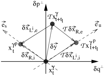
Figure 4: PSS at ${\bf x}_{t}$ right after part ${\cal L}$ and before ${\cal R}$. The displacement vector $\delta\vec{y}$ points from the orbit $\gamma$ to its time–reversed version $\gamma^{i}$. The deviation of the partner orbit $\gamma^{p}$ from the original orbit $\gamma$ is described by the vector $\delta\vec{x}_{R,i}$. Shown is only a two–dimensional projection of the $(2f-2)$-dimensional PSS.

Let us denote by $\delta\vec{x}_{{\cal R},i}$ the phase–space displacement between $\gamma$ and $\gamma^{p}$ at the beginning of part ${\cal R}$ (time $t$), see Fig. 4. To simplify the notations, we do not write explicitly the dependence of the displacement vectors on ${\bf x}^{\gamma}_{t}$ and $t_{\rm l}$. At the end of part ${\cal R}$, i.e., at time $t+t_{\rm l}$, the displacement $\delta\vec{x}_{{\cal R},i}$ has changed to $\delta\vec{x}_{{\cal R},e}$. At the beginning and the end of part ${\cal L}$, the displacement vectors between the time–reversed orbit $\gamma^{i}$ and the partner orbit $\gamma^{p}$ are denoted by $\delta\vec{x}_{{\cal L}^{i},i}$ and $\delta\vec{x}_{{\cal L}^{i},e}$, respectively. Here, ${\cal L}^{i}$ indicates that one has to invert time on ${\cal L}$. The vectors $\delta\vec{x}$ are given explicitly by

$$\delta\vec{x}_{{\cal R},i} = {\bf x}^{\gamma^{p}}_{t}-{\bf x}^{\gamma}_{t}\;,\quad\delta\vec{x}_{{\cal L}^{i},i}={\bf x}^{\gamma^{p}}_{t+t_{\rm l}}-{\mathcal{T}}{\bf x}^{\gamma}_{t}\;,\;$$ (33)

$$\delta\vec{x}_{{\cal R},e} = {\bf x}^{\gamma^{p}}_{t+t_{\rm l}}-{\bf x}^{\gamma}_{t+t_{\rm l}}\quad\text{and}\quad\delta\vec{x}_{{\cal L}^{i},e}={\bf x}^{\gamma^{p}}_{t}-{\mathcal{T}}{\bf x}^{\gamma}_{t+t_{\rm l}}\;.$$

The vectors $\delta\vec{x}_{{\cal R},i}$ and $\delta\vec{x}_{{\cal L}^{i},e}$ lie in the PSS defined at ${\bf x}^{\gamma}_{t}$ (see Fig. 4), while $\delta\vec{x}_{{\cal R},e}$ and $\delta\vec{x}_{{\cal L}^{i},i}$ are in the PSS at ${\bf x}^{\gamma}_{t+t_{\rm l}}$. Let $R=M(t_{\rm l},{\bf x}_{t}^{\gamma})$ and $L=M(T_{\gamma}-t_{\rm l},{\bf x}_{t+t_{\rm l}}^{\gamma})$ be the stability matrices of the parts ${\cal R}$ and ${\cal L}$ of $\gamma$, respectively. The stability matrix of ${\cal L}^{i}$ is given by $L^{i}={\mathcal{T}}\,L^{-1}\,{\mathcal{T}}$. Since the partner orbit $\gamma^{p}$ is assumed to follow closely $\gamma$ on part ${\cal R}$ and $\gamma^{i}$ on part ${\cal L}$, one can use the linear approximation to evaluate $\delta\vec{x}_{{\cal R},e}$ and $\delta\vec{x}_{{\cal L}^{i},e}$ as functions of $\delta\vec{x}_{{\cal R},i}$ and $\delta\vec{x}_{{\cal L}^{i},i}$, respectively, i.e.,

$$\delta\vec{x}_{{\cal R},e}=R\,\delta\vec{x}_{{\cal R},i}\quad,\quad\delta\vec{x}_{{\cal L}^{i},e}=L^{i}\,\delta\vec{x}_{{\cal L}^{i},i}.$$ (34a)

These equations determine the two single parts of the partner orbit $$\gamma^{p} {\cal R} {\cal L}$$ during and . In addition, the relations

$$\delta\vec{x}_{{\cal R},i}-\delta\vec{x}_{{\cal L}^{i},e}=\delta\vec{y}\quad,\quad\delta\vec{x}_{{\cal R},e}-\delta\vec{x}_{{\cal L}^{i},i}=-{\mathcal{T}}\delta\vec{y}\;$$ (34b)

make sure that the two parts fit together in the encounter region. The set of equations (34) can be rewritten to give

$$(1-L^{i}R)\,\delta\vec{x}_{{\cal R},i}=(1+L^{i}{\mathcal{T}})\,\delta\vec{y}\qquad\text{and}\qquad(1-RL^{i})\,\delta\vec{x}_{{\cal L}^{i},i}=({\mathcal{T}}+R)\,\delta\vec{y}\;.$$ (35)

Assuming that the determinants of $(1-L^{i}R)$ and $(1-RL^{i})$ do not vanish, the system of linear equations (34) has a unique solution. This solution yields the vectors $\delta\vec{x}$ in terms of the displacement $\delta\vec{y}$. Hence it characterizes the geometry of the partner orbit $\gamma^{p}$ in terms of deviations from $\gamma$ and $\gamma^{i}$.

It is important to note that all points ${\bf x}_{t+\Delta t}^{\gamma}$ within the encounter region lead to the same partner orbit $\gamma^{p}$. This means that, when writing Eqs. (34) for position ${\bf x}_{t+\Delta t}^{\gamma}$ instead of ${\bf x}_{t}^{\gamma}$, the solution is just the vector $\delta\vec{x}_{{\cal R},i}$ corresponding to ${\bf x}_{t}^{\gamma}$ shifted along the orbit during time $\Delta t$ and similarly for the other vectors $\delta\vec{x}$ in Eq. (33). To see this, let us first remark that the time evolution of $\delta\vec{y}$ between $t$ and $t+\Delta t$ is determined by the stability matrix $M=M(\Delta t,{\bf x}_{t}^{\gamma})$ via $\delta\vec{y}_{\Delta t}=M\delta\vec{y}$. Similar relations hold for the vectors $\delta\vec{x}$ in Eq. (33). The linearization of the equation of motion is, by definition, justified within the whole encounter region. The replacement of $({\bf x}_{t}^{\gamma},t_{\rm l})$ by $({\bf x}_{t+\Delta t}^{\gamma},t_{\rm l}-2\Delta t)$ thus amounts to the transformations

$$\begin{array}[]{clclclc}\delta\vec{y}&\to&\,M\,\delta\vec{y}&\quad,&&&\\ \delta\vec{x}_{{\cal R},i}&\to&\,M\,\delta\vec{x}_{{\cal R},i}&\quad,&\delta\vec{x}_{{\cal R},e}&\to&\,(M^{\prime})^{-1}\,\delta\vec{x}_{{\cal R},e}\;,\\ \delta\vec{x}_{{\cal L}^{i},i}&\to&\,(M^{i})^{-1}\,\delta\vec{x}_{{\cal L}^{i},i}&\quad,&\delta\vec{x}_{{\cal L}^{i},e}&\to&\,(M^{\prime})^{i}\,\delta\vec{x}_{{\cal L}^{i},e}\;,\\ R&\to&\,(M^{\prime})^{-1}\,R\,M^{-1}&\quad,&L&\to&\,M\,L\,M^{\prime}\,,\end{array}$$ (36)

with $M^{\prime}=M(\Delta t,{\bf x}_{t+t_{\rm l}^{\gamma}-\Delta t})$. One can easily check that the set of equations (34) is invariant under these transformations. This means that the same partner orbit $\gamma^{p}$ is obtained no matter whether ${\bf x}_{t}^{\gamma}$ or ${\bf x}_{t+\Delta t}^{\gamma}$ was chosen within the encounter region.

Let us first restrict our considerations to the case of long parts ${\cal R}$ and ${\cal L}$. This has to be understood in the sense that the linear approximation with respect to the evolution of $\delta\vec{y}$ breaks down at some time between $t$ and $t+t_{\rm l}$ and similarly, going backward in time, between $t$ and $t+t_{\rm l}-T_{\gamma}$. This means that $t_{\rm l}>\Delta t_{u}$ and $T_{\gamma}-t_{\rm l}>\Delta t_{s}$. We first note that these two conditions actually imply the stronger restriction

$$2\Delta t_{u}<t_{\rm l}<T_{\gamma}-2\Delta t_{s}\;$$ (37)

because the displacements $\delta\vec{y}$ at the beginning and the end of parts ${\cal R}$ and ${\cal L}$ are related to each other via the time–reversal operator ${{\mathcal{T}}}$. Formally this can be seen as follows. The displacement $\delta\vec{y}_{\Delta t}=\delta\vec{y}({\bf x}_{t+\Delta t}^{\gamma},t_{\rm l}-2\Delta t)$ satisfies $\delta\vec{y}_{t_{\rm l}-\Delta t}=-{\mathcal{T}}\delta\vec{y}_{\Delta t}$, as is easily checked with Eq. (II.4). Let us imagine that $\Delta t_{u}>t_{\rm l}/2$ implying that the linear approximation $\delta\vec{y}_{\Delta t}=M\delta\vec{y}$ is still valid after ${\bf x}_{t+\Delta t}^{\gamma}$ reaches the middle of ${\cal R}$. This would imply that $|\delta\vec{y}_{\Delta t}|$ continues to increase exponentially with $\Delta t$ after time $t_{\rm l}/2$ until $\Delta t$ reaches $\Delta t_{u}$. Such a statement is in contradiction with the above–mentioned identity. This shows that $\Delta t_{u}<t_{\rm l}/2$ must hold. A similar argument on part ${\cal L}$ shows the second inequality in Eq. (37).

For a long part ${\cal R}$ fulfilling (37), the stability matrix $R$ in Eq. (34a) is characterized by exponentially large stretching factors $\Lambda_{i}({\bf x}_{t}^{\gamma},t_{\rm l})$. Substituting Eq. (II.4) into Eq. (35) and using Eq. (28), one thus finds

$$\begin{array}[]{lllll}\delta\vec{x}_{{\cal R},i}&=&\delta\vec{y}_{s}&=&\sum\limits_{i=1}^{f-1}s_{i}\;\vec{e}^{\,s}_{i}({\bf x}^{\gamma}_{t})\;,\\ \delta\vec{x}_{{\cal L}^{i},i}&=&{\mathcal{T}}\delta\vec{y}_{u}&=&\sum\limits_{i=1}^{f-1}u_{i}\;\vec{e}^{\,s}_{i}({\mathcal{T}}{\bf x}^{\gamma}_{t})\;,\\ \delta\vec{x}_{{\cal R},e}&=&-{\mathcal{T}}\delta\vec{y}_{s}&=&-\sum\limits_{i=1}^{f-1}s_{i}\;\vec{e}^{\,u}_{i}({\mathcal{T}}{\bf x}^{\gamma}_{t})\;,\\ \delta\vec{x}_{{\cal L}^{i},e}&=&-\delta\vec{y}_{u}&=&-\sum\limits_{i=1}^{f-1}u_{i}\;\vec{e}^{\,u}_{i}({\bf x}^{\gamma}_{t})\;.\end{array}$$ (38)

This solution is correct up to first order in the small quantities $s_{i}$ and $u_{i}$. Terms smaller than $s_{i}$ and $u_{i}$ by a factor $e^{-t_{\rm l}\lambda_{i}^{\gamma}}$ or $e^{-(T_{\gamma}-t_{\rm l})\lambda_{i}^{\gamma}}$ have been also neglected. It means that due to the large lengths of both parts ${\cal R}$ and ${\cal L}$ the vectors $\delta\vec{x}_{{\cal R},i}$ and ${\mathcal{T}}\delta\vec{x}_{{\cal L}^{i},i}$ describing the partner orbit have to lie very close to the stable and the unstable manifolds at ${\bf x}_{t}^{\gamma}$, respectively Braun02b . Furthermore, the points ${\bf x}_{t}^{\gamma}$, ${\bf x}_{t}^{\gamma^{p}}$, ${\mathcal{T}}{\bf x}_{t+t_{\rm l}}^{\gamma}$, and ${\mathcal{T}}{\bf x}_{t+t_{\rm l}}^{\gamma^{p}}$ form a parallelogram in phase space Spehner03 ; Turek03 , see Fig. 4.

It is important to notice that there can be a small set of vectors $\delta\vec{y}$ for which (37) does not hold. This is the case when either of the parts, say ${\cal R}$, is too short Spehner03 ; Turek03 ; Mueller03 . Then the orbit $\gamma$ and the time–reversed orbit $\gamma^{i}$ stay close together inside the whole part ${\cal R}$ so that ${\cal R}$ is contained within the encounter region. This means that ${\cal R}$ is an almost self–retracing part of trajectory in configuration space. This may happen, for example, in billiards with hard walls if one of the reflections is almost perpendicular to the boundary Mueller01 ; Mueller03 . If there is no potential or hard wall, as in the case of the geodesic flow on a Riemann surface with constant negative curvature Sieber01 ; Sieber02 , trajectories with almost self–retracing parts cannot exist. If ${\cal R}$ is contained within the encounter region, the linear approximation $\delta\vec{y}_{\Delta t}=M(\Delta t,{\bf x}_{t}^{\gamma})\delta\vec{y}$ can be applied to $\delta\vec{y}=\delta\vec{y}({\bf x}_{t}^{\gamma},t_{\rm l})$ at least up to $\Delta t=t_{\rm l}$. This leads to the additional equation $R\,\delta\vec{y}=-{\mathcal{T}}\delta\vec{y}$ besides Eq. (34). For indeed, following the linearized motion around ${\cal R}$, we see that ${\bf x}_{t}$ and ${\mathcal{T}}{\bf x}_{t+t_{\rm l}}$ are interchanged and reverted in time. The solution (35) is then $\delta\vec{x}_{{\cal R},i}=\delta\vec{y}$, $\delta\vec{x}_{{\cal R},e}=-{\mathcal{T}}\delta\vec{y}$ and $\delta\vec{x}_{{\cal L}^{i},i}=\delta\vec{x}_{{\cal L}^{i},e}=\vec{0}$. This means that if the time $t_{\rm l}$ violates the condition (37), the solution of Eq. (34) does not yield a new partner orbit but just the time–reversed orbit $\gamma^{i}$. Since the orbit pairs $(\gamma,\gamma^{i})$ are already accounted for in the diagonal approximation (19) one must only consider intersection points $\delta\vec{y}({\bf x}_{t}^{\gamma};t_{\rm l})$ in the PSS which fulfill (37). In other words, the length $t_{\rm l}$ of part ${\cal R}$ must be large enough so that the linear approximation for $\delta\vec{y}_{\Delta t}$ breaks down for $\Delta t<t_{\rm l}$ and similarly for part ${\cal L}$. Note that $\Delta t_{s}$ and $\Delta t_{u}$ are large (of order $\lambda_{j}^{-1}\ln|s_{j}^{-1}|$ and $\lambda_{k}^{-1}\ln|u_{k}^{-1}|$, respectively, see Subsection II.4) if the components $\{s_{i},u_{i}\}$ of $\delta\vec{y}$ are small.

II.6 Action difference, orbit weights, and Maslov indices

The action difference $\Delta S$ between the orbit $\gamma$ and its partner orbit $\gamma^{p}$ can be found by expanding the action of $\gamma^{p}$ in part ${\cal R}$ in terms of $\gamma$ and in part ${\cal L}$ in terms of $\gamma^{i}$. The derivation of $\Delta S$ is the same as for systems with $f=2$ degrees of freedom Spehner03 ; Turek03 . By using the parallelogram property (38), which is justified since $t_{\rm l}>2\Delta t_{u}$ and $T_{\gamma}-t_{\rm l}>2\Delta t_{s}$ are large, one finds that $\Delta S$ is given in terms of the components $\{s_{i},u_{i}\}$ of the displacement $\delta\vec{y}({\bf x}_{t}^{\gamma},t_{\rm l})$ by

$$\Delta S\equiv S_{\gamma}-S_{\gamma^{p}}\approx\delta\vec{y}_{u}^{\,T}\,\Sigma\,\delta\vec{y}_{s}=\sum\limits_{j=1}^{f-1}S_{\text{cl}}s_{j}u_{j}\equiv\sum\limits_{j=1}^{f-1}S_{j}\,.$$ (39)

Thus $\Delta S$ equals the symplectic area of the parallelogram introduced in Subsection II.5, see Fig. 4. In the last two equalities in Eq. (39), we have used Eqs. (27b, II.4) and defined $S_{j}\equiv S_{\text{cl}}s_{j}u_{j}$. The approximation (39) is correct up to second order in the small $|s_{i}|,|u_{i}|\ll 1$. It is consistent with the concept of the encounter region as it yields the same action difference no matter at what position ${\bf x}_{t+\Delta t}^{\gamma}$ within the encounter region it is evaluated. This is due to the conservation of the symplectic product under the dynamics. As only small action differences $\Delta S\sim\hbar$ contribute significantly to the semiclassical form factor (16), the restriction of the considerations presented above to small components $|s_{i}|,|u_{i}|\sim\sqrt{\hbar/S_{\rm cl}}\ll 1$ is well justified.

Besides the two different actions $S_{\gamma}$ and $S_{\gamma^{p}}$ entering the semiclassical form factor (16), one must also compare the weights $w_{\gamma}$ and $w_{\gamma^{p}}$ given by Eq. (14). These weights are equal up to small corrections of first order in $u_{i}$ and $s_{i}$ as can be shown in the following way. First of all, for any continuous function $f({\bf x})$ defined in phase space one finds, using Eq. (32),

$$\int\limits_{0}^{T_{\gamma^{p}}}{\rm d}t^{\prime}\,f({\bf x}^{\gamma^{p}}_{t^{\prime}})\simeq\int\limits_{t}^{t+t_{\rm l}}{\rm d}t^{\prime}\,f({\bf x}^{\gamma}_{t^{\prime}})+\int\limits_{t+t_{\rm l}}^{T_{\gamma}+t}{\rm d}t^{\prime}\,f({\cal T}{\bf x}^{\gamma}_{2t+t_{\rm l}-t^{\prime}})$$ (40)

with small corrections of the order of $|s_{i}|,|u_{i}|\sim\sqrt{\hbar/S_{\rm cl}}$. That means that the integral over any function $f({\bf x})$ along the partner orbit $\gamma^{p}$ is approximately given by integrals along parts of $\gamma$ and $\gamma^{i}$. The corrections in Eq. (40) are primarily due to the deviations of the partner orbit $\gamma^{p}$ from the original orbit $\gamma$ or its time–reversed version $\gamma^{i}$ within the encounter region. Obviously, Eq. (40) yields $T_{\gamma}\simeq T_{\gamma^{p}}$ for $f({\bf x})=1$. Similarly, we can apply Eq. (40) to the local growth rates $f({\bf x})=\chi_{i}({\bf x})$, which results into $\lambda_{i}^{\gamma}\simeq\lambda_{i}^{\gamma^{p}}$ in view of Eq. (24) and of the identity $\chi_{i}({\mathcal{T}}{\bf x})=\chi_{i}({\bf x})$. Hence the Lyapunov exponents of the two partner orbits $\gamma$ and $\gamma^{p}$ have to be almost equal. Finally, we can also identify $f({\bf x})$ with the local change in the winding number of the stable or unstable manifolds which allows for a calculation of the Maslov indices Foxman95 . As the winding number of a periodic orbit has to be an integer one finds that, for smooth dynamics, the Maslov index of the partner orbit has to be exactly equal to the Maslov index of the original orbit Turek03 ; Mueller03 , i.e., $\mu_{\gamma}=\mu_{\gamma^{p}}$. Putting these results together in Eq. (14), one concludes that $w_{\gamma}\simeq w_{\gamma^{p}}$. In the spirit of a stationary phase approximation we therefore keep only the action difference $\Delta S=S_{\gamma}-S_{\gamma^{p}}$ in the phase while neglecting small differences in the pre-exponential factors in Eq. (16).

II.7 Statistics of partner orbits and the spectral form factor

In the following we show how the orbit pairs $(\gamma,\gamma^{p})$ specified above determine the next-to-leading-order result for the spectral form factor. We assume that the dominant terms beyond the diagonal approximation in Eq. (16) are due to the systematic action correlations of these orbit pairs. Thus the double sum over periodic orbits (16) can be replaced by a single sum over the orbits $\gamma$ followed by a sum over all the partner orbits $\gamma^{p}$ of $\gamma$ while all other terms are neglected, i.e.,

$$K^{(2)}(T)=\frac{T}{T_{H}}\,\left\langle\left\langle\sum_{\text{partners $\gamma^{p}$}}\exp\left({\rm{i}}\frac{S_{\gamma}-S_{\gamma^{p}}}{\hbar}\right)\right\rangle_{\text{po},T}\right\rangle_{\Delta E}$$ (41)

where the periodic–orbit average over $\gamma$ is given by Eq. (17). All partner orbits $\gamma^{p}$ of $\gamma$ are characterized by the set of action differences $\{S_{j}\}$ defined in Eq. (39). Therefore, setting $\tau=T/T_{H}$, the sum over the partner orbits in Eq. (41) can be rewritten as an integral over the $S_{j}$’s,

$$K^{(2)}(\tau)=\tau\left\langle\int\limits_{-S_{\rm max}(E)}^{S_{\rm max}(E)}{\rm d}S_{1}\dots\rm dS_{f-1}\,\left\langle\frac{{\rm d}^{f-1}N_{\gamma}(\{S_{j}\})}{{\rm d}S_{1}\dots\rm dS_{f-1}}\right\rangle_{{\rm po},\tau T_{H}}\exp\left({\rm i}\sum\limits_{j=1}^{f-1}\frac{S_{j}}{\hbar}\right)\right\rangle_{\Delta E}\,,$$ (42)

where $S_{\rm max}$ stands for the maximal action difference occurring among the pairs of partner orbits. The density of partner orbits $\gamma^{p}$ for a given orbit $\gamma$ with the set of action differences $\{S_{j}\}$ is denoted by ${\rm d}^{f-1}N_{\gamma}(\{S_{j}\})/{\rm d}S_{1}\dots\rm dS_{f-1}$. This quantity is the crucial ingredient, and we will show how its periodic–orbit average can be calculated in ergodic systems with an arbitrary number of degrees of freedom. In contrast to the case of two–dimensional systems, the derivation is significantly more involved because of the higher number of stable and unstable coordinates, Lyapunov exponents, and the maximum condition (II.4).

Let us for a moment fix one point ${\bf x}$ on $\gamma$ (to simplify the notation, we omit here the superscript $\gamma$ on ${\bf x}$ and choose temporarily the origin of time such that ${\bf x}_{t}={\bf x}$ for $t=0$), and consider the PSS ${\mathcal{P}}$ perpendicular to the orbit at ${\bf x}$. The time–reversed orbit $\gamma^{i}$ pierces through ${\mathcal{P}}$ many times. Some of these piercings — each of it associated with a different time $t_{\rm l}$ — occur at points ${\cal T}{\bf x}_{t_{\rm l}}$ close to ${\bf x}$, see Figs. 3 and 5. Let $\rho_{\gamma}(\{s_{i},u_{i}\};{\bf x})\,{\rm{d}}^{f-1}s\,{\rm{d}}^{f-1}u$ denote the number of such intersection points, with stable and unstable components of $\delta\vec{y}={\cal T}{\bf x}_{t_{\rm l}}-{\bf x}$ lying in intervals $(s_{i},s_{i}+{\rm{d}}s_{i})$ and $(u_{i},u_{i}+{\rm{d}}u_{i})$, respectively. We exclude from $\rho_{\gamma}$ all points ${\cal T}{\bf x}_{t_{\rm l}}$ violating the condition $2\Delta t_{u}<t_{\rm l}<T_{\gamma}-2\Delta t_{s}$ since they either do not exist at all or do not give rise to a distinct partner orbit. Thus we have the density of valid intersection points,

$$\rho_{\gamma}(\{s_{i},u_{i}\};{\bf x})=\int\limits_{2\Delta t_{u}}^{T_{\gamma}-2\Delta t_{s}}{\rm d}t_{\rm l}\,\delta\left([{\bf x}-{\mathcal{T}}{\bf x}_{t_{\rm l}}]_{\parallel}\right)\prod\limits_{i=1}^{f-1}\delta\left([{\bf x}-{\mathcal{T}}{\bf x}_{t_{\rm l}}]_{u,i}-u_{i}\right)\delta\left([{\bf x}-{\mathcal{T}}{\bf x}_{t_{\rm l}}]_{s,i}-s_{i}\right).$$ (43)

Here, the first delta function ensures that ${\cal T}{\bf x}_{t_{\rm l}}$ lies in ${\mathcal{P}}$, i.e., that the coordinate $[{\bf x}-{\mathcal{T}}{\bf x}_{t_{\rm l}}]_{\parallel}$ of ${\bf x}-{\mathcal{T}}{\bf x}_{t_{\rm l}}$ in the direction parallel to the orbit vanishes. The lower indices $s$ and $u$ indicate the stable and unstable components of the vectors inside the square brackets.

Figure 5: Sketch of the PSS as it is shifted along the periodic orbit $\gamma$ (solid line). Three pieces of the time–reversed orbit $\gamma^{i}$ are represented by dashed lines. If the PSS moves with the flow in phase space from ${\bf x}_{t1}^{\gamma}$ to ${\bf x}_{t2}^{\gamma}$ all intersection points of the PSS with $\gamma^{i}$ change their positions according to the linearized equations of motion (20). Note that not only $\gamma^{i}$ but also $\gamma$ itself could come close to ${\bf x}_{t1}^{\gamma}$ at a later time. However, we have not include this in the sketch above.

In order to determine how many partner orbits $\gamma^{p}$ of a given fixed orbit $\gamma$ exist with a given set of action differences $\{S_{i}\}$, one has to count the number of corresponding encounter regions of $\gamma$. As explained in the beginning of this section each of these encounter regions can be associated to a displacement vector $\delta\vec{y}$ or to its corresponding time–evolved $\delta\vec{y}_{\Delta t}$, $-\Delta t_{s}\leq\Delta t\leq\Delta t_{u}$. Therefore we consider the dynamics within the PSS ${\cal P}_{t}$ at ${\bf x}_{t}^{\gamma}$. It can be parametrized by means of the stable and unstable coordinates of the different vectors $\delta\vec{y}({\bf x}_{t}^{\gamma},t_{\text{l}})$ associated to different times $t_{\text{l}}$. As the PSS is shifted following the phase–space flow along the orbit $\gamma$, the stable and unstable coordinates of each such vector change leaving only the products $S_{j}=S_{\rm cl}\,s_{j}u_{j}$ invariant. The vector $\delta\vec{y}_{\Delta t}=\delta\vec{y}_{\Delta t}({\bf x}_{t},t_{\text{l}})\in{\cal P}_{t+\Delta t}$ corresponding to a fixed $t_{\text{l}}$ thus moves, as ${\cal P}_{t+\Delta t}$ is shifted by increasing $\Delta t$, on a hyperbola as long as ${\bf x}_{t+\Delta t}^{\gamma}$ remains within the encounter region, i.e., for $-\Delta t_{s}\leq\Delta t\leq\Delta t_{u}$, see Fig. 6. Since the number of partner orbits is equal to the number of encounter regions one has now to count each encounter region exactly once. This can be achieved in two alternative ways:

1. One can measure the flux of vectors $\delta\vec{y}$ through the hypersurface defining the end of the encounter region (see Fig. 6). According to the definition of the encounter region given in Subsection II.4, this hypersurface consists of the faces $\partial\,{\cal C}_{j}^{\pm}=\{(s_{i},u_{i}):|s_{i}|\leq c,|u_{i}|\leq c,u_{j}=\pm c\}$, $j=1,\ldots,f-1$, of the hypercube ${\cal C}=\{(s_{i},u_{i}):|s_{i}|\leq c,|u_{i}|\leq c\}$. The union of all these faces defines a $(2f-3)$-dimensional closed hypersurface $\partial\,{\cal C}$ contained in the $(2f-2)$-dimensional PSS. The corresponding flux is obtained by multiplying the density $\rho_{\gamma}$ with the component $\dot{u}_{j}$ of the velocity of the vector $\delta\vec{y}$ in the direction normal to $\partial\,{\cal C}_{j}^{\pm}$. This velocity is given by $\dot{u}_{j}=\chi_{j}({\bf x}_{t}^{\gamma})\,c$, see Eq. (26). Integrating along the orbit we obtain

   $$\frac{{\rm d}^{f-1}N_{\gamma}(\{S_{i}\})}{{\rm d}S_{1}\dots\rm dS_{f-1}} = \int\limits_{0}^{T_{\gamma}}{\rm d}t\;\sum\limits_{j=1}^{f-1}\;\int\limits_{-c}^{c}{\rm d}^{f-1}s\;{\rm d}^{f-1}u\;\rho_{\gamma}(\{s_{i},u_{i}\};{\bf x}^{\gamma}_{t})\;\chi_{j}({\bf x}^{\gamma}_{t})\,c$$ (44)

   $$\qquad\times\Bigl{(}\delta(u_{j}-c)+\delta(u_{j}+c)\Bigr{)}\;\left(\prod\limits_{i=1}^{f-1}\delta(S_{\text{cl}}s_{i}u_{i}-S_{i})\right).$$

   The last product of delta functions restricts the action differences to the values $\{S_{i}\}$. It should be noted that, since the local growth rate $\chi_{j}({\bf x}_{t}^{\gamma})$ can take negative values for some times $t$, the vector $\delta\vec{y}$ may also re-enter into the hypercube ${\cal C}$ through some face $\partial\,{\cal C}_{k}^{\pm}$ with a negative normal velocity $\dot{u}_{k}=\chi_{k}({\bf x}_{t}^{\gamma})\,c$ (with possibly $k\not=j$). However, since $\delta\vec{y}$ increases exponentially with time at large times, there is one more passing of $\delta\vec{y}$ through $\partial\,{\cal C}$ in the outwards direction ($\dot{u}>0$) than in the inwards direction ($\dot{u}<0$). The contributions of all subsequent passings then mutually cancel each other in Eq. (44). Hence, for each encounter region, only the first crossing of $\partial\,{\cal C}$ at time $\Delta t=\Delta t_{u}$ is accounted for, as required. Let us also mention that if we had taken any other closed hypersurface contained in the hypercube ${\cal C}$ instead of $\partial\,{\cal C}$ the same result would have been obtained. This is because the dynamics conserves the number of points in phase space and thus the number of vectors $\delta\vec{y}$.

2. An alternative version of Eq. (44), treating all points within the encounter region on equal footing, can be found as follows. Every vector $\delta\vec{y}$ is counted as long as it remains within the hypercube ${\cal C}$. Therefore one has to include the additional factor of $1/t_{\rm enc}$, since per definition (31), $t_{\rm enc}$ is approximately the time each vector $\delta\vec{y}$ spends within that hypercube. The density of partner orbits (44) can thus be rewritten as

   $$\frac{{\rm d}^{f-1}N_{\gamma}(\{S_{i}\})}{{\rm d}S_{1}\dots\rm dS_{f-1}}\simeq\int\limits_{0}^{T_{\gamma}}{\rm d}t\;\int\limits_{-c}^{c}{\rm d}^{f-1}s\,{\rm d}^{f-1}u\,\frac{\rho_{\gamma}(\{s_{i},u_{i}\};{\bf x}^{\gamma}_{t})}{t_{\rm enc}(\{s_{i},u_{i}\};{\bf x}^{\gamma}_{t})}\left(\prod\limits_{i=1}^{f-1}\delta(S_{\text{cl}}s_{i}u_{i}-S_{i})\right).$$ (45)

   More precisely, this expression can be derived as follows (also see the Appendix A). Consider first only the contribution of the encounters at ${\bf x}_{t}^{\gamma}$ after time $t_{\rm l}-2t$, for a fixed $t_{\rm l}$ and an arbitrary time $t$. The time duration $t_{\text{enc}}$ of the encounter and the product $u_{i}s_{i}$ of the stable and unstable components of the vector $\delta\vec{y}({\bf x}_{t}^{\gamma},t_{\rm l}-2t)$ are independent of $t$ as long as ${\bf x}_{t}^{\gamma}$ stays within an encounter region, i.e., while $s_{i}$ and $u_{i}$ vary within $(-c,c)$. The time spent by the point characterized by $\delta\vec{y}({\bf x}_{t}^{\gamma},t_{\rm l}-2t)$ within the hypercube ${\cal C}$ is approximately equal to $t_{\text{enc}}$ in the limit $|u_{i}|,|s_{i}|\sim\sqrt{\hbar/S_{\text{cl}}}\ll 1$, where $t_{\text{enc}}$ is large (of order $\ln\hbar$). Indeed, although possible re-entrances of $\delta\vec{y}$ into ${\cal C}$ (see above) may increase the total time spent by $\delta\vec{y}$ inside ${\cal C}$ to a value greater than $t_{\text{enc}}$, the relative error made by approximating it by $t_{\text{enc}}$ is small. Using also the fact that the above–specified encounter regions are disjoint (if they were overlapping they would define one bigger region), it follows that the r.h.s. of Eq. (45) gives approximately the density of those encounter regions with respect to the action differences $\{S_{i}\}$. The result (45) then follows by integrating $t_{\rm l}$ over all possible values.

Figure 6: Schematic drawing of a projection of the Poincaré surface of section (PSS). The flow of intersection points (black filled circles) is represented by the thin arrows. For long enough time the unstable component $u_{j}$ grows while the stable component $s_{j}$ shrinks with $S_{j}=S_{\text{cl}}s_{j}u_{j}$ being constant. There are two ways to count the intersection points. Either the flux through the $u_{j}=c$ surface (dotted line) is considered, as in Eq. (44), or one counts the number of points in the volume of the encounter region (dashed area) and normalizes that by the time each point spends in there, as in Eq. (45).

Actually, expressions (44) and (45) are equivalent. Using the fact that the number of vectors $\delta\vec{y}$ is conserved by the dynamics, one can transform the integrals over the hypersurface $\partial\,{\cal C}$ into an integral over the entire volume of the hypercube. More details on this proof of the equality between Eq. (44) and Eq. (45) are given in the Appendix A. It is important for what follows to note that this equality still holds if the range of integration of $t_{\rm l}$ in Eq. (43) is replaced by the larger interval $(0,T_{\gamma})$ which corresponds to the additional inclusion of intersection points $\delta\vec{y}$ that cannot be associated with a partner orbit. The reason for the introduction of the two different expressions for the number of partner orbits is because of its crucial importance from a technical point of view. We will apply either Eq. (44) or Eq. (45) depending on which one can be calculated easier. It will turn out that this allows for a major simplification of the derivations to follow. In particular, the complicated analytic structure of $t_{\text{enc}}(\{s_{i},u_{i}\};{\bf x})$, see Eqs. (II.4) and (31), does not directly enter the calculations.

The periodic–orbit average of the density of partner orbits in Eq. (44) or Eq. (45) can be transformed into an average over the constant–energy surface by means of the sum rule (18). After this step has been performed, the density $\rho_{\gamma}$ has to be evaluated at arbitrary points ${\bf x}$ on a set of measure one inside the constant–energy surface, instead of taking the points ${\bf x}_{t}^{\gamma}$ belonging to periodic orbits as the arguments. For such points ${\bf x}$ one can neglect classical correlations between ${\bf x}$ and ${\cal T}{\bf x}_{t_{\rm l}}$ for $2\Delta t_{u}\leq t_{\rm l}\leq T-2\Delta t_{s}$. This is because $\lambda_{i}^{-1}\ll\Delta t_{u,s}\ll T$ in the relevant limit $|s_{i}|,|u_{i}|\sim\sqrt{\hbar/S_{\rm cl}}\ll 1$, $T\sim T_{H}\sim\hbar^{1-f}$. More precisely, ergodicity allows one to approximate the time integral in Eq. (43) by a phase–space average,

$$\rho(\{s_{i},u_{i}\};{\bf x}) \approx \frac{T-2\Delta t_{s}(\{s_{i}\};{\bf x})-2\Delta t_{u}(\{u_{i}\};{\bf x})}{\Omega}\int{\rm{d}}{\bf x}^{\prime}\,\delta(E-H({\bf x}^{\prime}))\,\delta\left([{\bf x}-{\mathcal{T}}{\bf x}^{\prime}]_{\parallel}\right)$$ (46)

$$\prod\limits_{i=1}^{f-1}\delta\left([{\bf x}-{\mathcal{T}}{\bf x}^{\prime}]_{u,i}-u_{i}\right)\delta\left([{\bf x}-{\mathcal{T}}{\bf x}^{\prime}]_{s,i}-s_{i}\right)\;.$$

Since the Jacobian of the transformation $(\delta{\bf q}^{\perp},\delta{\bf p}^{\perp})\to(s_{i},u_{i})$ gives a factor $S_{\text{cl}}^{f-1}$ this yields

$$\rho(\{s_{i},u_{i}\};{\bf x}) \approx \rho^{\rm lead}+\rho^{\rm corr}(\{s_{i},u_{i}\};{\bf x})$$

$$= \frac{S^{f-1}_{\rm cl}}{\Omega}T-\frac{S^{f-1}_{\rm cl}}{\Omega}\,2t_{\rm enc}(\{s_{i},u_{i}\};{\bf x})\;.$$

Therefore $\rho$ is given by a leading contribution plus a small correction term due to the exclusion of short times $t_{l}$ violating condition (37). The corrections to the ergodic approximation are not written in Eqs. (46) and (II.7). Although they may be bigger than $\rho^{\text{corr}}$, one expects them to be strongly reduced after averaging ${\bf x}$ over the constant–energy surface, as required by the sum rule. This is not the case for the correction term $\rho^{\text{corr}}$, which, as we shall see now, determines the form factor.

Indeed, if only the leading term $\rho^{\rm lead}$ in the density (II.7) is considered, one finds that the form factor (42) vanishes in the semiclassical limit for the following reason. As $\rho^{\rm lead}$ does not depend on ${\bf x}$ and $\{s_{i},u_{i}\}$, its contribution to the density of partner orbits can be most easily calculated by means of Eq. (44). It yields

$$\left\langle\frac{{\rm d}^{f-1}N_{\gamma}(\{S_{i}\})}{{\rm d}S_{1}\dots\rm dS_{f-1}}\right\rangle_{{\rm po},T}^{\rm(lead)}\approx 2^{f-1}\;\frac{T^{2}}{\Omega}\;\sum\limits_{j=1}^{f-1}\lambda_{j}\;\prod\limits_{i\neq j}^{f-1}\ln\left(\frac{S_{\text{cl}}c^{2}}{|S_{i}|}\right).$$ (48)

Here we have used the identity $\overline{\chi_{j}({\bf x})}=\lambda_{j}$. If this result (48) is inserted into the expression for the form factor (42), one obtains $K^{(2)}(\tau)=0$ due to the energy average.

Therefore the small correction term $\rho^{\rm corr}$ given in Eq. (II.7) is of crucial importance. To determine its contribution to the form factor, it turns out to be technically favorable to use expression (45) instead of Eq. (44) for the density of partner orbits. The reason is that the two appearances in Eqs. (45) and (II.7) of $t_{\rm enc}$ mutually cancel. Inserting $\rho^{\rm corr}$ from Eq. (II.7) into Eq. (45), one finds

$$\left\langle\frac{{\rm d}^{f-1}N_{\gamma}(\{S_{i}\})}{{\rm d}S_{1}\dots\rm dS_{f-1}}\right\rangle_{{\rm po},T}^{\rm(corr)}=-2^{f}\,\frac{T}{\Omega}\,\prod\limits_{i=1}^{f-1}\ln\left(\frac{S_{\text{cl}}c^{2}}{|S_{i}|}\right)\;.$$ (49)

The result (48) together with Eq. (49) gives the correct asymptotic form of the averaged density of partners in the limit $\hbar\to 0$, $\tau=T/T_{H}$ fixed. Since the leading term (48) gives a vanishing contribution to the form factor (42), only the correction (49) determines the final result,

$$K^{(2)}(\tau)\simeq-2\tau^{2}\frac{T_{H}}{\Omega}\prod\limits_{i=1}^{f-1}\left\{-2\int\limits_{-\infty}^{\infty}{\rm d}S_{i}\,\exp\left({\rm i}\frac{S_{i}}{\hbar}\right)\,\ln\left(\frac{|S_{i}|}{S_{\text{cl}}c^{2}}\right)\right\}\simeq-2\tau^{2}\,.$$ (50)

This result is universal, i.e., it does not contain any information about the set of Lyapunov exponents $\{\lambda_{i}\}$ or the constant $c$ defining the encounter region. Thus as our first major result we find that the next-to-leading order correction beyond the diagonal approximation agrees with the BGS conjecture independently of the number of degrees of freedom the system possesses.

III Matrix elements fluctuations

The aim of this section is to evaluate the generalized form factor $K_{ab}(T)$ defined in Eq. (4) based on the method developed in the previous section. This form factor describes the correlations of the diagonal matrix elements $\langle n|\hat{a}|n\rangle$ and $\langle m|\hat{b}|m\rangle$, corresponding to distinct energies $E_{n}$ and $E_{m}$, of two given quantum observables $\hat{a}$ and $\hat{b}$. We assume that $\hat{a}$ and $\hat{b}$ have well–behaved classical limits given by smooth Weyl symbols $a({\bf x})$ and $b({\bf x})$.

III.1 Leading term

To zeroth order in $\hbar$, the form factor (4) is given by

$$K_{ab}(T)\approx\overline{a({\bf x})}\;\overline{b({\bf x})}\,K(T)\;.$$ (51)

Actually, Snirelman’s theorem Snirelman74 for classical ergodic flows implies that the Wigner functions of almost all eigenstates $|n\rangle$ with energies $E_{n}$ converging to $E$ are uniformly distributed over the constant–energy surface $H({\bf x})=E$ in the semiclassical limit. Equivalently, this means that the matrix elements $\langle n|\hat{a}|n\rangle$ converge to the average (7),

$$\langle n|\hat{a}|n\rangle\to\overline{a({\bf x})}$$

$$\text{as}\quad\hbar\to 0\;,\quad n\to\infty\quad\text{such that}\quad E_{n}\approx E\;.$$ (52)

It is worthwhile to mention that this is only true for eigenstates $|n\rangle$ of the quantum Hamiltonian pertaining to a “set of density one” . Heller’s scars Heller84 are prominent examples of “exceptional” eigenstates violating Eq. (III.1). Choosing, e.g., a Gaussian weight of width $\Delta E$ in the energy average in Eq. (2), one can express $K_{ab}(T)$ for $T>\Delta T/2$ as

$$K_{ab}(T) = \frac{1}{\langle d(E)\rangle_{\Delta E}}\frac{1}{\sqrt{2\pi\Delta E^{2}}}\sum_{n,m}\langle n|\hat{a}|n\rangle\langle m|\hat{b}|m\rangle e^{-\frac{{\rm{i}}}{\hbar}(E_{m}-E_{n})T}\,h(E_{m}-E_{n})$$ (53)

$$\times\,\exp\left(-\frac{(E_{n}+E_{m}-2E)^{2}}{8\Delta E^{2}}\right)\,.$$

Since all functions of $E_{n}$ and $E_{m}$ vary noticeably on the scale $\Delta E\gg\langle d(E)\rangle^{-1}_{\Delta E}$, the eigenstates not belonging to the “set of density one”, such as scars, have a negligible contribution to the sum in Eq. (53). One can then replace $\langle n|\hat{a}|n\rangle\langle m|\hat{b}|m\rangle$ by the product $\overline{a({\bf x})}\;\overline{b({\bf x})}$ and move this factor out of the sum. This yields Eq. (51), which is therefore a direct consequence of Snirelman’s theorem.

To obtain information on matrix element fluctuations, one thus needs to study the semiclassical corrections (next term in power of $\hbar$) to the leading behavior (51) of the form factor. Let us define

$$\hat{a}^{\prime}=\hat{a}-\overline{a({\bf x})}\hat{1}\;\;\mbox{ , }\;\;\hat{b}^{\prime}=\hat{b}-\overline{b({\bf x})}\hat{1}\,,$$ (54)

so that the associated Weyl symbols $a^{\prime}({\bf x})$ and $b^{\prime}({\bf x})$ average to zero. Then the form factor $K_{ab}(T)$ is related to $K_{a^{\prime}b^{\prime}}(T)$ by the formula

$$K_{ab}(T) - \overline{a({\bf x})}\;\overline{b({\bf x})}\,K(T)=$$

$$K_{a^{\prime}b^{\prime}}(T)+\overline{a({\bf x})}\,K_{1b^{\prime}}(T)+\overline{b({\bf x})}\,K_{a^{\prime}1}(T)\,.$$

Comparing with Eq. (51), one sees that the r.h.s. of Eq. (III.1) vanishes as $\hbar\to 0$. The purpose of the two next subsections is to estimate the first term of the r.h.s., which turns out to be proportional to $1/T_{H}={\mathcal{O}}(\hbar^{f-1})$. We start with the diagonal contribution of pairs of identical orbits (modulo time–reversal) to $K_{a^{\prime}b^{\prime}}(T)$ and then include the pairs of correlated orbits $(\gamma,\gamma^{p})$ studied in Section II. We restrict our derivation to the case of observables with vanishing mean, i.e., $\overline{a({\bf x})}=\overline{b({\bf x})}=0$ so that $a=a^{\prime}$ and $b=b^{\prime}$. Therefore we shall not be concerned further in this paper with the second and third terms in Eq. (III.1).

III.2 Correction term within the diagonal approximation

Let us first consider the semiclassical correction to the leading term (51) within the diagonal approximation. This correction has been already studied in Refs. Eckhardt95 ; EFKAMM95 ; Eckhardt97 ; Eckhardt00 . However, we will argue below that the results of Refs. Eckhardt95 ; EFKAMM95 ; Eckhardt97 ; Eckhardt00 can only be applied to observables $a({\bf x})$ or $b({\bf x})$ independent of the momentum ${\bf p}$. We treat here the more general case of smooth observables $a$ and ${b}$ depending on both the position ${\bf q}$ and the momentum ${\bf p}$, by following the lines of Subsection IIC of Ref. EFKAMM95 .

Retaining only the contribution of those pairs obtained by pairing each orbit with itself or with its time–reversed version in the double sum (16), the semiclassical form factor can be written as

$$K_{ab}^{\text{(1)}}(T)=\frac{1}{T_{H}}\left\langle\int_{0}^{T_{\gamma}}\frac{{\rm d}t}{T_{\gamma}}\,a({\bf x}^{\gamma}_{t})\,\left(\int_{0}^{T_{\gamma}}{\rm d}t^{\prime\prime}\,b({\bf x}^{\gamma}_{t^{\prime\prime}})+\int_{0}^{T_{\gamma}}{\rm d}t^{\prime\prime}\,b({\mathcal{T}}{\bf x}^{\gamma}_{t^{\prime\prime}})\right)\right\rangle_{\text{po},T}\,.$$ (56)

Substituting $t^{\prime}=t^{\prime\prime}-t$ and using the periodicity of $\gamma$ yields

$$K_{ab}^{\text{(1)}}(T)=\frac{2}{T_{H}}\int_{0}^{T}{\rm d}t\,\left\langle\int_{0}^{T_{\gamma}}\frac{{\rm d}t^{\prime}}{T_{\gamma}}\,a({\bf x}^{\gamma}_{t})b^{S}({\bf x}^{\gamma}_{t+t^{\prime}})\right\rangle_{\text{po},T}$$ (57)

with $b^{S}({\bf x})$ as given in Eq. (9).

We now assume that the classical dynamics is sufficiently chaotic so that the time–correlation function (9) of the classical observables $a({\bf x})$ and $b^{S}({\bf x})$ decays faster than $1/t$ to zero. In strongly chaotic systems all classical correlation functions of smooth observables decay exponentially, as a result of a gap in the spectrum of the resonances of the Frobenius–Perron operator (all resonances but the one corresponding to the Liouville measure are contained inside a circle of radius strictly smaller than unity) Gaspard98 . The mixing property makes sure that the time–correlation function $C_{ab}^{S}(t)$ tends to zero in the large-$t$ limit, but is still not strong enough for our purpose: it does not imply that $C_{ab}^{S}(t)$ can be integrated from $0$ to $\infty$.

Applying the sum rule (18) to Eq. (57) gives

$$K_{ab}^{\text{(1)}}(T)\simeq\frac{2}{T_{H}}\int_{0}^{\infty}{\rm d}t^{\prime}\,C_{ab}^{S}(t^{\prime})\;$$ (58)

in the limit $\hbar\to 0$ with $\tau=T/T_{H}$ fixed. If $a({\bf x})$ or $b({\bf x})$ is a function of the position ${\bf q}$ only, then $a^{S}({\bf x})=a({\bf x})$ or $b^{S}({\bf x})=b({\bf x})$, respectively. As a result, $C_{ab}^{S}(t)=C_{ab}(t)$. In such a case, Eq. (58) coincides with the result of Refs. Eckhardt95 and  EFKAMM95 . In the opposite case, the mean $C_{ab}^{S}(t)$ of the correlation function of $a({\bf x})$ and $b({\bf x})$ and the correlation function of $a({\bf x})$ and $b({\cal T}{\bf x})$ must be considered.

As noted in Ref. EFKAMM95 , some chaotic systems which fulfill the mixing property, such as the symmetric stadium billiard, exhibit algebraic decays of correlations in $1/t$. Then the integral in Eq. (58) diverges and the form factor $K_{ab}^{(1)}$ is of order $T_{H}^{-1}\ln T_{H}$ instead of $T_{H}^{-1}$.

Let us also mention that, for chaotic dynamics, the integrals $\int_{0}^{T}{\rm d}t\,a({\bf x}_{t})$ and $\int_{0}^{T}{\rm d}t\,b^{S}({\bf x}_{t})$ of the observables $a({\bf x})$ and $b^{S}({\bf x})$ along pieces of (nonperiodic) trajectories of time $T$, thought as function of the initial point ${\bf x}$, may be often considered as Gaussian random variables with respect to the Liouville measure for large $T$’s Gaspard98 . These random variables have a system–specific covariance $2T\int_{0}^{\infty}{\rm d}t\,C_{ab}^{S}(t)$, which is thus also related to the fluctuations of the diagonal matrix elements of $\hat{a}$ and $\hat{b}$ as given by $K_{ab}(T)$.

III.3 Contribution of the partner orbits

The contribution of the partner orbits to the semiclassical form factor (16) is obtained by inserting the product $A_{\gamma}\,B_{{\gamma}^{p}}$ of the integrals of the classical observable $a({\bf x})$ along $\gamma$ and of the observable $b({\bf x})$ along $\gamma^{p}$ in front of the exponential in Eq. (41). The forthcoming calculation is simplified by noting that if ${\gamma}^{p}$ is a partner orbit of $\gamma$, then its time–reversed version ${\gamma}^{p,i}$ is also a partner orbit of $\gamma$, with the same action. This is because if one exchanges the role of parts ${\cal R}$ and ${\cal L}$ in the definition (32), the corresponding partner orbit is just ${\gamma}^{p,i}$. As a result, one may equivalently insert $A_{\gamma}(B_{{\gamma}^{p}}+B_{{\gamma}^{p,i}})/2$ in front of the exponential in Eq. (41), instead of $A_{\gamma}\,B_{{\gamma}^{p}}$. The mean $(B_{{\gamma}^{p}}+B_{{\gamma}^{p,i}})/2$ is the integral of the symmetrized observable $b^{S}({\bf x})$ given by Eq. (9) along $\gamma^{p}$. It can be estimated by applying Eq. (40) to $b^{S}({\bf x})$ and using $b^{S}({\bf x})=b^{S}({\mathcal{T}}{\bf x})$ together with the periodicity of $\gamma$. This yields

$$\frac{1}{2}\left(B_{{\gamma}^{p}}+B_{{\gamma}^{p,i}}\right)\simeq\int_{0}^{T_{\gamma}}\frac{{\rm d}t^{\prime\prime}}{T_{\gamma}}\,b^{S}({\bf x}_{t^{\prime\prime}}^{\gamma})\;$$ (59)

and reflects the fact that the two orbits $\gamma$ and $\gamma^{i}$ explore almost the same phase–space regions as the two partner orbits $\gamma^{p}$ and $\gamma^{p,i}$. Hence the generalization of Eq. (42) reads

$$K_{ab}^{(2)}(\tau)=\tau \left\langle\int\limits_{-S_{\text{max}}(E)}^{S_{\text{max}}(E)}{\rm d}S_{1}\dots\rm dS_{f-1}\,\left\langle\frac{{\rm d}^{f-1}N_{\gamma}(\{S_{i}\})}{{\rm d}S_{1}\dots\rm dS_{f-1}}\int_{0}^{T_{\gamma}}\frac{{\rm d}t^{\prime}}{T_{\gamma}}\int_{0}^{T_{\gamma}}\frac{{\rm d}t^{\prime\prime}}{T_{\gamma}}\,a({\bf x}_{t^{\prime}}^{\gamma})b^{S}({\bf x}_{t^{\prime}+t^{\prime\prime}}^{\gamma})\right\rangle_{{\rm po},\tau T_{H}}\right.$$ (60)

$$\left.\times\exp\left({\rm i}\sum\limits_{i=1}^{f-1}\frac{S_{i}}{\hbar}\right)\right\rangle_{\Delta E}\;.$$

By using Eq. (44) and substituting $t^{\prime}\to t^{\prime\prime\prime}=t^{\prime}-t$ before applying the sum rule (18), one finds that the leading contribution $\rho^{\text{lead}}$ to the density in Eq. (II.7) yields

$$\displaystyle\left\langle\frac{{\rm d}^{f-1}N_{\gamma}(\{S_{i}\})}{{\rm d}S_{1}\dots\rm dS_{f-1}}\int_{0}^{T_{\gamma}}\frac{{\rm d}t^{\prime}}{T_{\gamma}}\int_{0}^{T_{\gamma}}\frac{{\rm d}t^{\prime\prime}}{T_{\gamma}}\,a({\bf x}_{t^{\prime}}^{\gamma})b^{S}({\bf x}_{t^{\prime}+t^{\prime\prime}}^{\gamma})\right\rangle_{{\rm po},T}^{\text{(lead)}}\qquad\qquad\qquad\qquad$$ (61)

$$\displaystyle\approx\frac{2^{f-1}}{\Omega}\sum_{j=1}^{f-1}\prod_{i\not=j}^{f-1}\ln\left(\frac{S_{\text{cl}}c^{2}}{|S_{i}|}\right)\ \int_{0}^{T}{\rm d}t^{\prime\prime\prime}\int_{0}^{T}{\rm d}t^{\prime\prime}\,\overline{\chi_{j}({\bf x})\,a({\bf x}_{t^{\prime\prime\prime}})b^{S}({\bf x}_{t^{\prime\prime\prime}+t^{\prime\prime}})}\;.$$

Employing ergodicity, the integral over $t^{\prime\prime\prime}$ can be approximated by a phase–space average and yields $T\,\overline{\chi_{j}({\bf x})}\int_{0}^{\infty}{\rm{d}}t^{\prime\prime}\,C_{ab}^{S}(t^{\prime\prime})$. Thus inserting Eq. (61) into Eq. (60) gives $K_{ab}^{(2)}(\tau)=0$. As in Section II, the contribution to the form factor of $\rho^{\text{lead}}$ thus vanishes. By using Eq. (45), we obtain the contribution of the small correction term $\rho^{\text{(corr)}}$ in Eq. (II.7),

$$\displaystyle\left\langle\frac{{\rm d}^{f-1}N_{\gamma}(\{S_{i}\})}{{\rm d}S_{1}\dots\rm dS_{f-1}}\int_{0}^{T_{\gamma}}\frac{{\rm d}t^{\prime}}{T_{\gamma}}\int_{0}^{T_{\gamma}}\frac{{\rm d}t^{\prime\prime}}{T_{\gamma}}\,a({\bf x}_{t^{\prime}}^{\gamma})b^{S}({\bf x}_{t^{\prime}+t^{\prime\prime}}^{\gamma})\right\rangle_{{\rm po},T}^{\text{(corr)}}\qquad\qquad$$

$$\displaystyle\approx-2^{f}\frac{1}{\Omega T}\prod_{i=1}^{f-1}\ln\left(\frac{S_{\text{cl}}c^{2}}{|S_{i}|}\right)\int_{0}^{T}{\rm d}t^{\prime\prime\prime}\int_{0}^{T}{\rm d}t^{\prime\prime}\,\overline{a({\bf x}_{t^{\prime\prime\prime}})b^{S}({\bf x}_{t^{\prime\prime\prime}+t^{\prime\prime}})}$$ (62)

since the dependence on $t_{\text{enc}}(\{s_{i},u_{i}\};{\bf x})$ in Eq. (45) and Eq. (II.7) mutually cancels. The average $\overline{a({\bf x}_{t^{\prime\prime\prime}})b^{S}({\bf x}_{t^{\prime\prime\prime}+t^{\prime\prime}})}$ equals the correlation function $C_{ab}^{S}(t^{\prime\prime})$. It follows from Eq. (50) that, as $\hbar\to 0$,

$$K_{ab}^{(2)}(\tau)\approx-2\tau\,\frac{1}{T_{H}}\int_{0}^{\infty}{\rm d}t\,C_{ab}^{S}(t)\;.$$ (63)

Remarkably, one obtains for the leading off-diagonal contribution the same result as for the diagonal approximation, with $2$ replaced by $-2\tau$ as in the spectral form factor. In particular this means that the classical correlations enter in exactly the same way via the correlation function $C_{ab}^{S}(t)$. Assuming that only identical orbits modulo time–reversal symmetry and pairs of partner orbits $(\gamma,\gamma^{p})$ contribute to the semiclassical form factor (16) up to order $\tau^{2}$ included, this yields

$$K_{ab}(\tau)\approx\frac{1}{\tau\;T_{H}}\Bigl{(}K(\tau)+{\mathcal{O}}(\tau^{3})\Bigr{)}\int_{0}^{\infty}{\rm d}t\,C_{ab}^{S}(t)$$ (64)

as announced in the introduction. This result holds if the correlation function $C_{ab}^{S}(t)$ decays faster than $1/t$ as $t\to\infty$, in order that the upper integration limit $T=\tau T_{H}$ may be replaced by $\infty$. It is valid for observables $\hat{a}$ and $\hat{b}$ such that $\overline{a({\bf x})}=\overline{b({\bf x})}=0$ only.

If $\overline{a({\bf x})}\not=0$ or $\overline{b({\bf x})}\not=0$, Eq. (III.1) must be used and the second and third terms in the r.h.s. of this equation have to be estimated. Repeating the above calculation for these terms, one finds that both vanish in zeroth order in $\hbar$, thus being in accordance with Snirelman’s theorem. For instance, within the diagonal approximation, Eq. (56) gives $K_{a^{\prime}1}^{(1)}(T)=2T_{H}^{-1}\langle\int_{0}^{T_{\gamma}}{\rm{d}}t\,a^{\prime}({\bf x}_{t}^{\gamma})\rangle_{\text{po},T}\approx 2\tau\,\overline{a^{\prime}({\bf x})}$, which is zero since $\overline{a^{\prime}({\bf x})}=0$. The leading contribution in $\hbar$ is thus governed by the finite–time corrections to the sum rule (18). Similarly, replacing $a$ by $a^{\prime}$ and $b$ by $1$ in Eq. (III.3), the second integral in the second member becomes $T\,\overline{a^{\prime}({\bf x})}$, which means that $K_{a^{\prime}1}^{(2)}(T)\approx 0$ up to higher–order corrections in the sum rule. One concludes that our method does not allow us to estimate $K_{a^{\prime}1}$ as $\hbar\to 0$ beyond the leading order in $\hbar$. For systems with exponential decay of classical correlation functions, it is not irreasonable to expect that the finite–time corrections to the sum rule (18) are exponentially small in $T$. In such a case $K_{a^{\prime}1}$ and $K_{1b^{\prime}}$ would be negligible with respect to $K_{a^{\prime}b^{\prime}}$, which is of order $\hbar^{f-1}$ by Eq. (64).

IV Summary and outlook

In this work we presented a semiclassical evaluation of the generalized form factor $K_{ab}(\tau)$ going beyond the diagonal approximation. We first considered the spectral form factor $K(\tau)=K_{11}(\tau)$ for systems with more than two degrees of freedom, i.e., $f\geq 2$. We proved that the leading contribution due to pairs of periodic orbits with correlated actions is independent of $f$ in agreement with the RMT prediction. An important step in our calculation was to show the equivalence between the two different approaches for counting partner orbits which were independently developed in Ref. Turek03 and Refs. Spehner03 ; Heusler03 for two–dimensional systems. Based on these results for the spectral form factor we then investigated the generalized form factor $K_{ab}(\tau)$. In this case we were able to show a universal dependence of $K_{ab}(\tau)$ on the rescaled time $\tau$. Furthermore, we found that the contribution of the partner orbits depends on the classical time–correlation function $C_{ab}^{S}(t)$ in exactly the same way as in the diagonal approximation, see Eq. (64). An interesting open question is to prove (or disprove) that this is still the case at higher orders in $\tau$ or even for arbitrary large $\tau>1$. In such a case one could get rid of the error term ${\cal O}(\tau^{3})$ added to $K(\tau)$ in Eq. (64).

Our semiclassical treatment of the generalized form factor beyond the diagonal approximation can in principle be extended to other physical observables containing matrix elements in chaotic systems. This includes expressions where transition matrix elements play a role Wilk87 ; Mehlig98 (e.g., dipole excitations in quantum dots MR98 ), and linear response functions for mesoscopic systems Ric00 with applications to transport, magnetism, or optical response. So far, nearly all semiclassical approaches to such quantities have been relying on the diagonal approximation, as long as additional averages are involved. A notable exception is the calculation of the weak localization correction to the conductance in Ref. Ric02 , showing an important contribution of the partner orbits. It would thus be of great interest to study the corrections to the diagonal approximation in the various response functions appearing in mesoscopic physics.

Acknowledgments: We acknowledge support from the Deutsche Forschungsgemeinschaft (Ri 681/5 and SFB/TR 12). We are grateful to B. Eckhardt and U. Smilansky for interesting discussions. SM also thanks P. Braun, F. Haake, and S. Heusler for close cooperation.

*

Appendix A Transformation of the surface integral into a volume integral

In this appendix we prove the equality of the two different approaches for counting the partner orbits based on Eq. (44) and Eq. (45), respectively. To this end we show that an equality of the general structure

$$\int\limits_{0}^{T}{\rm d}t\,\int\limits_{\cal V}{\rm d}V_{\delta\vec{y}}\;\frac{\varrho(\delta\vec{y},t)}{t_{\cal V}(\delta\vec{y},t)}\;=\;\int\limits_{0}^{T}{\rm d}t\,\int\limits_{\partial{\cal V}_{\rm out}}{\rm d}\vec{A}_{\delta\vec{y}}\;\varrho(\delta\vec{y},t)\;\dot{\delta\vec{y}}(\delta\vec{y},t)\,$$ (65)

holds under the conditions which are relevant for the statistics of the number of partners. Here, $\delta\vec{y}$ is a vector in a multidimensional space, e.g., the $(2f-2)$-dimensional PSS. The volume element in this space is given by ${\rm d}V_{\delta\vec{y}}={\rm d}^{f-1}u\,{\rm d}^{f-1}s$ while ${\rm d}\vec{A}_{\delta\vec{y}}$ characterizes the surface element. The left hand side of Eq. (65) thus contains an integral over any $(2f-2)$-dimensional volume ${\cal V}$ in the PSS. Inside ${\cal V}$ we follow the time evolution of a density field $\varrho(\delta\vec{y},t)$; the corresponding velocity field is denoted by ${\dot{\delta\vec{y}}}(\delta\vec{y},t)$. As Eq. (65) is applied to the PSS following a periodic orbit of length $T$, we can assume periodicity such that $\varrho(\delta\vec{y},t)=\varrho(\delta\vec{y},t+T)$ and $\dot{\delta\vec{y}}(\delta\vec{y},t)=\dot{\delta\vec{y}}(\delta\vec{y},t+T)$. Due to current conservation the density is constant along the flow, i.e., $\varrho(\delta\vec{y},0)=\varrho(\delta\vec{y}_{t},t)$ or $\dot{\varrho}(\delta\vec{y}_{t},t)=0$. The time $t_{\cal V}(\delta\vec{y},t)$ in Eq. (65) is defined as the total time a point spends in the volume ${\cal V}$ if it starts at time $t$ at position $\delta\vec{y}$ and moves until time $t+T$. If the volume ${\cal V}$ is chosen to coincide with the hypercube ${\cal C}$ defining the encounter region, see Subsection II.4, then $t_{\cal V}$ is approximately equal to the time $t_{\text{enc}}$, Eq. (31). The surface of ${\cal V}$ is decomposed as $\partial{\cal V}=\partial{\cal V}_{\rm in}+\partial{\cal V}_{\rm out}$. Here, $\partial{\cal V}_{\rm in/out}$ stands for that part of the total surface through which the flux defined by $\varrho$ and $\dot{\delta\vec{y}}$ enters or leaves ${\cal V}$ in the long–time limit, respectively. More precisely speaking, the total flux between time $0$ and $T$ through any piece of $\partial{\cal V}_{\rm out}$ must be positive.

For the proof of relation (65) let us first consider the case where the total density $\varrho(\delta\vec{y},t)$ is given by a single point starting at $\delta\vec{y}_{0}$, i.e., $\varrho_{1}(\delta\vec{y},t)=\delta(\delta\vec{y}-\delta\vec{y}_{t})$. Then the time $t_{\cal V}$ is given as

$$t_{\cal V}(\delta\vec{y}_{t},t) = \int\limits_{t}^{t+T}{\rm d}t^{\prime}\;\Theta_{\cal V}(\delta\vec{y}_{t^{\prime}})=\int\limits_{0}^{T}{\rm d}t^{\prime}\;\int\limits_{\cal V}{\rm d}V_{\delta\vec{y\,^{\prime}}}\;\varrho_{1}(\delta\vec{y\,}^{\prime},t^{\prime})$$ (66)

$$= t_{\cal V}(\delta\vec{y}_{0},0)\;,$$

where $\Theta_{\cal V}(\delta\vec{y})$ equals $1$ if $\delta\vec{y}\in{\cal V}$ and zero otherwise. In Eq. (66) we made use of the periodicity of the motion. We then obtain for the left hand side of Eq. (65)

$$\int\limits_{0}^{T}{\rm d}t \int\limits_{\cal V}{\rm d}V_{\delta\vec{y}}\;\frac{\varrho_{1}(\delta\vec{y},t)}{t_{\cal V}(\delta\vec{y},t)}=$$

$$\frac{1}{t_{\cal V}(\delta\vec{y}_{0},0)}\int\limits_{0}^{T}{\rm d}t\,\int\limits_{\cal V}{\rm d}V_{\delta\vec{y}}\;\varrho_{1}(\delta\vec{y},t)=1\,.$$

In close analogy we thus find that if the single point density is replaced by $\varrho(\delta\vec{y},t)=\sum_{i}\varrho_{i}(\delta\vec{y},t)$ which represents an arbitrary number $n$ of points given by their initial conditions then the left hand side of Eq. (65) just gives the total number of particles $n$ that pass ${\cal V}$ during one period. But this is exactly what the right hand side of Eq. (65) gives. It just measures the outgoing flux through the surface of $\cal V$ between time $0$ and $T$ which also yields the total number of particles $n$ because the particle number is conserved.

Finally we also note that the density $\varrho(\delta\vec{y},t)$ is not restricted to a sum of $\delta$ functions. Each of these $\delta$ functions can also be multiplied with any function $g(\delta\vec{y},t)$ that is constant when following the flow within ${\cal V}$, i.e., $g(\delta\vec{y}_{0},0)=g(\delta\vec{y}_{t},t)$. In the context of Subsection II.7, $g$ could, for example, be any function of the action difference as in Eqs. (44) and (45). In this case the density $\varrho$ entering Eq. (65) can be considered as a weighted density $\varrho=\rho\,g$.

If all local unstable growth rates $\chi_{k}({\bf x})$ are non-negative one can directly identify $t_{\cal V}=t_{\text{enc}}$ and thus the equality (65) means that Eq. (44) exactly equals Eq. (45). On the other hand, if these local unstable growth rates assume negative values in certain areas of the phase space then this implies that the unstable components of a displacement vector can also decrease on short time scales. This would lead to a multiple entry of the same point into the ’encounter region’ characterized by ${\cal V}={\cal C}$. In this case the relation (65) means that Eq. (45) is asymptotically equal to Eq. (44) as the length $t_{\text{enc}}$ becomes large so that $|t_{\cal V}-t_{\text{enc}}|\ll t_{\text{enc}}$ or similarly $t_{\cal V}\simeq t_{\text{enc}}$.

References

- (1) O. Bohigas, M.J. Giannoni, and C. Schmit, Phys. Rev. Lett. 52, 1 (1984).
- (2) H.-J. Stöckmann, Quantum Chaos: An Introduction (Cambridge University Press, Cambridge, 1999).
- (3) F. Haake, Quantum Signatures of Chaos (Springer, Berlin, 2000).
- (4) M.C. Gutzwiller, Chaos in Classical and Quantum Mechanics (Springer, New York, 1990).
- (5) M.V. Berry, Proc. R. Soc. London, Ser. A 400, 229 (1985).
- (6) M. Sieber and K. Richter, Physica Scripta T90, 128 (2001).
- (7) M. Sieber, J. Phys. A: Math. Gen. 35, 613 (2002).
- (8) D. Spehner, J. Phys. A: Math. Gen. 36, 7269 (2003).
- (9) M. Turek and K. Richter, J. Phys. A: Math. Gen. 36, L455 (2003).
- (10) S. Müller, Eur. Phys. J. B 34, 305 (2003).
- (11) S. Müller, S. Heusler, P. Braun, F. Haake, and A. Altland, Phys. Rev. Lett. 93, 014103 (2004).
- (12) B. Eckhardt and J. Main, Phys. Rev. Lett. 75, 2300 (1995).
- (13) B. Eckhardt, S. Fishman, J. Keating, O. Agam, J. Main, and K. Müller, Phys. Rev. E 52, 5893 (1995).
- (14) B. Eckhardt, Physica D 109, 53 (1997).
- (15) B. Eckhardt, S. Fishman, and I. Varga, Phys. Rev. E 62, 7867 (2000).
- (16) R.E. Prange, Phys. Rev. Lett. 78, 2280 (1997).
- (17) A.I. Snirelman, Ups. Mat. Nauk 29, 87 (1974); S. Zelditch, Duke Math. J. 55, 919 (1987); Y. Colin de Verdière, Commun. Math. Phys. 102, 497 (1985); B. Helffer, A. Martinez, and D. Robert, Commun. Math. Phys. 109, 313 (1987).
- (18) N.L. Balazs and B.K. Jennings, Phys. Rep. 104, 347, (1984).
-
(19)
B. Eckhardt, S. Fishman, K. Müller, and D. Wintgen,
Phys. Rev. A 45, 3531 (1992);
P. Gaspard, D. Alonso, and I. Burghardt, Adv. Chem. Phys. 90, 105 (1995). - (20) M. Combescure, J. Ralston, and D. Robert, Commun. Math. Phys. 202, 463 (1999).
- (21) H. Primack and U. Smilansky, Phys. Rep. 327, 1 (2000).
- (22) E.B. Bogomolny and J.P. Keating, Phys. Rev. Lett. 77, 1472 (1996).
- (23) W. Parry and M. Pollicott, Zeta functions and the periodic orbit structure of hyperbolic dynamics, Astérisque 187-188, 1 (1990).
- (24) J.H. Hannay and A.M. Ozorio de Almeida, J. Phys. A: Math. Gen. 17, 3429 (1984).
- (25) S. Heusler, S. Müller, P. Braun, and F. Haake, J. Phys. A: Math. Gen. 37, L31 (2004).
- (26) P. Gaspard, Chaos, Scattering and Statistical Mechanics (Cambridge University Press, Cambridge, England, 1998).
- (27) P. Braun, F. Haake, and S. Heusler, J. Phys. A: Math. Gen. 35, 1381 (2002).
- (28) S. Müller, Diplomarbeit, Universität Essen (2001).
- (29) J.A. Foxman and J.M. Robbins, J. Phys. A: Math. Gen. 30, 8187 (1997).
- (30) E.J. Heller, Phys. Rev. Lett. 53, 1515 (1984).
- (31) B. Mehlig, Phys. Rev. E 59, 390 (1998).
- (32) B. Mehlig and K. Richter, Phys. Rev. Lett. 80, 1936 (1998).
- (33) M. Wilkinson, J. Phys. A 20, 2415 (1987).
- (34) K. Richter, Semiclassical Theory of Mesoscopic Quantum Systems (Springer, Berlin, 2000).
- (35) K. Richter and M. Sieber, Phys. Rev. Lett. 89, 206801-1 (2002).