Localization of nonlinear excitations in curved waveguides

Abstract

Motivated by the example of a curved waveguide embedded in a photonic crystal, we examine the effects of geometry in a “quantum channel” of parabolic form. We study the linear case and derive exact as well as approximate expressions for the eigenvalues and eigenfunctions of the linear problem. We then proceed to the nonlinear setting and its stationary states in a number of limiting cases that allow for analytical treatment. The results of our analysis are used as initial conditions in direct numerical simulations of the nonlinear problem and localized excitations are found to persist, as well as to have interesting relaxational dynamics. Analogies of the present problem in contexts related to atomic physics and particularly to Bose-Einstein condensation are discussed.

I Introduction

Localization phenomena are widely recognized as key to understanding the excitation dynamics in many physical contexts such as light propagation, charge and energy transport in condensed-matter physics and biophysics, and Bose-Einstein condensation of dilute atomic gases [1, 2]. Recent advances in micro-structuring technology have made it possible to fabricate various low-dimensional systems with complicated geometry. Examples are photonic crystals with embedded defect structures such as microcavities, waveguides and waveguide bends [2, 3, 4, 5], narrow structures (quantum dots and channels) formed at semiconductor heterostructures [6, 7, 8], magnetic nanodisks, dots and rings [9, 10, 11].

On the other hand, it is well known that the wave equation subject to Dirichlet boundary conditions has bound states in straight channels of variable width [12, 13, 14], and in curved channels of constant cross-section [15, 16]. Spectral and transport characteristics of quantum electron channels [17] and waveguides in photonic crystal [3] are in essential ways modified by the existence of segments with finite curvature. The two-dimensional Laplacian operator supported by an infinite curve which is asymptotically straight has at least one bound state below the threshold of the continuum spectrum, as was recently proved in [18]. The appearance of an effective attractive potential in the wave equation is due to constraining quantum particles from higher to lower dimensional manifolds [19, 20, 21]. Curvature induced bound-state energies and and corresponding wave functions were studied in [22].

Until recently there have been few theoretical and numerical studies of the effect of curvature on properties of nonlinear excitations. Nonlinear whispering gallery modes for a nonlinear Maxwell equation in microdisks were investigated in [23]; the excitation of whispering-gallery-type electromagnetic modes by a moving fluxon in an annular Josephson junction was shown in [24]. Nonlinear localized modes in two-dimensional photonic crystal waveguides were studied in [25]. A curved chain of nonlinear oscillators was considered in [26] and it was shown that the interplay of curvature and nonlinearity leads to a symmetry breaking when an asymmetric stationary state becomes energetically more favorable than a symmetric stationary state. Propagation of Bose-Einstein condensates in magnetic waveguides was experimentally demonstrated quite recently in [27]; single-mode propagation was observed along homogeneous segments of the waveguide, while geometric deformations of the microfabricated wires led to strong transverse excitations.

Motivated by the experimental relevance of the above mentioned geometric deformations, in the present work we aim at investigating nonlinear excitations in a prototypical setup incorporating such phenomena. As our case example, we will examine an infinitely narrow curved nonlinear waveguide (channel) embedded in two-dimensional linear medium (idle region).

Our presentation will proceed as follows: in Section II, we set up the mathematical model of interest and examine its general properties and equations of motion. In Section III, we study the linear case and present its explicit solutions for the bound states, as well as for the corresponding eigenvalues. In section IV, we focus on the nonlinear problem, while in section V we supplement our analysis with numerical results. Finally, in section VI, we summarize our findings and present our conclusions. The appendix presents some additional technical details on the solution of the linear problem and its Green’s function formulation.

II System and Equations of Motion

Our model is described by the Hamiltonian

$$H=\int\limits_{-\infty}^{\infty}\{|\nabla\psi|^{2}-\nu\,(|\psi|^{2}-A\frac{1}{2}|\psi|^{4})\,\delta(y-f(x))\}dxdy,$$ (1)

where $\psi(\vec{r},t)$ is the complex amplitude function, $\vec{r}=(x,y)$, $\nabla^{2}=\partial_{x}^{2}+\partial_{y}^{2}$, $\nu$ is the energy difference between the quantum channel and the passive region (refractive index difference in the case of photonic crystals and waveguides), the coefficient $A$ characterizes the nonlinearity of the medium, e.g., the nonlinear corrections to the refractive index of the photonic band-gap materials, or self-interaction of the quasi-particles in the quantum channel. The function $y=f(x)$ gives the shape of the channel. From the Hamiltonian, we obtain the equation of motion in the form

$$i\partial_{t}\psi(\vec{r},t)+\nabla^{2}\psi+\nu\,\delta(y-f(x))F(|\psi|^{2})\,\psi=0,$$ (2)

where the function $F(|\psi|^{2})$ is given by

$$F=1-A|\psi|^{2}.$$ (3)

Equation (2) has as integrals of motion the Hamiltonian (1) and the ($L^{2}$) norm (referred to e.g., as the number of atoms in BEC or power in nonlinear optics)

$$N=\int\limits_{-\infty}^{\infty}|\psi|^{2}\,dxdy.$$ (4)

It is well known (see e.g., [28]) that if the edges of the Frénet trihedron (the tangent, the principal normal and the binormal) at a given point are considered as the axes of a Cartesian coordinate system, then the equation of the curve in a neighbourhood of this point has the form

$$x=s+\cdots,~{}y=\frac{\kappa}{2}\,s^{2}+\cdots,~{}z=-\frac{\kappa\,\tau}{6}\,s^{3}+\cdots$$ (5)

where $s$ is the arclength, $\kappa$ is the curvature and $\tau$ is the torsion of the curve at this point. Thus if the curvature of the plane curve is not too large one can represent it as a parabola

$$y=\frac{\kappa}{2}\,x^{2}.$$ (6)

In this case Eq. (2) takes the form

$$i\partial_{t}\psi+\nabla^{2}\psi+\nu\,\delta(y-\frac{x^{2}}{2R})F(|\psi|^{2})\,\psi=0,$$ (7)

where $R=1/\kappa$ is the maximum radius of curvature of the curve. It is convenient to use the parabolic coordinates

$$x=\frac{uv}{R},~{}~{}~{}y=\frac{R}{2}+\frac{1}{2R}(u^{2}-v^{2}).$$ (8)

The coordinate lines are two orthogonal families of confocal parabolas, with axes along the $y$ axis. These lines are given by

$$R\frac{x^{2}}{v^{2}}=2y-R+v^{2}/R,~{}~{}~{}R\frac{x^{2}}{u^{2}}=-2y+R+u^{2}/R$$

or

$$u/\sqrt{R}=\pm\sqrt{y-\frac{R}{2}+\sqrt{(y-\frac{R}{2})^{2}+x^{2}}},$$ (9)

$$v/\sqrt{R}=\sqrt{-y+\frac{R}{2}+\sqrt{(y-\frac{R}{2})^{2}+x^{2}}}.$$ (10)

The variable $u$ is allowed to range from $-\infty$ to $\infty$, whereas $v$ is positive. Introducing Eqs. (8) into Eq. (7) and using the properties of parabolic coordinates (see e.g., [29]), we obtain:

$$i\,\frac{1}{R^{2}}(u^{2}+v^{2})\,\partial_{t}\psi+\left(\partial_{u}^{2}+\partial_{v}^{2}\right)\psi+\nu\,\delta(v-R)\,F(|\psi|^{2})\,\psi=0.$$ (11)

Using the Fourier transform with respect to $t$,

$$\bar{\psi}=\frac{1}{2\pi}\int\limits_{-\infty}^{\infty}e^{i\omega t}\psi(u,v,t)\,dt,$$ (12)

where the bars denote the Fourier transformed quantities, one can represent Eq. (11) in the form

$$-\frac{\omega}{R^{2}}(u^{2}+v^{2})\,\bar{\psi}+\left(\partial_{u}^{2}+\partial_{v}^{2}\right)\bar{\psi}+\nu\,\delta(v-R)\,\overline{F(|\psi|^{2})\,\psi}(u,v)=0.$$ (13)

Equation (11) can, in turn, be expressed in the form of the integral equation

$$\bar{\psi}(u,v,\omega)=\nu\,\int\limits_{-\infty}^{\infty}du^{\prime}\,\int\limits_{0}^{\infty}\,dv^{\prime}\,G\left(u,v;u^{\prime},v^{\prime}\right)\,\delta(v^{\prime}-R)\,\overline{F(|\psi|^{2})\,\psi}(u^{\prime},v^{\prime},\omega),$$ (14)

where the Green’s function $G\left(u,v;u^{\prime},v^{\prime}\right)$ satisfies the equation

$$\left(\partial_{u}^{2}+\partial_{v}^{2}\right)\,G-\frac{\omega}{R^{2}}(u^{2}+v^{2})\,G=-\delta(u-u^{\prime})\,\delta(v-v^{\prime}),$$ (15)

and has the form (see Appendix for details)

$$G\left(u,v;u^{\prime},v^{\prime}\right)=\frac{\sqrt{\pi}}{2}\sum_{n=0}^{\infty}\,F_{n}(u)\,F_{n}(u^{\prime})\,\{V_{n}(v)\,U_{n}(v^{\prime})\,\theta(v^{\prime}-v)+U_{n}(v)\,V_{n}(v^{\prime})\,\theta(v-v^{\prime})\}.$$ (16)

Here

$$F_{n}(u)=a_{n}\,e^{-\sqrt{\omega}u^{2}/2R}\,H_{n}\left(u\,\omega^{1/4}\,R^{-1/2}\right),~{}~{}~{}n=0,1,2,...,$$ (17)

where $H_{n}\left(z\right)$ is the Hermite polynomial [30], $a_{n}=\left(\omega^{1/2}/R\,\pi\right)^{1/4}\,\left(2^{n}\,n!\right)^{-1/2}$ is the normalization constant, and

$$V_{n}(v)=V\left(n+\frac{1}{2},v\,\sqrt{2}\,\omega^{1/4}\,R^{-1/2}\right),$$ (18)

$$U_{n}(v)=\,U\left(n+\frac{1}{2},v\,\sqrt{2}\,\omega^{1/4}\,R^{-1/2}\right),$$ (19)

with $V(a,x)$ and $U(a,x)$ being the Weber parabolic cylinder functions [30].

It can then be seen from Eqs. (14) and (16) that the Fourier transformed channel wave function

$$\bar{\phi}(u,\omega)\equiv\bar{\psi}(u,v,\omega)\bigg{|}_{v=R},$$ (20)

satisfies the equation

$$\bar{\phi}(u,\omega)=\nu\,\omega^{-1/4}\,\frac{\sqrt{\pi\,R}}{2}\,\sum_{n=0}^{\infty}\,\int\limits_{-\infty}^{\infty}\,F_{n}(u)\,F_{n}(u^{\prime})\,V_{n}(R)\,U_{n}(R)\,\overline{F(|\phi|^{2})\,\phi}(u^{\prime},\omega)\,du^{\prime},$$ (21)

or equivalently the equation

$$\nu\,\omega^{-1/4}\,\frac{\sqrt{\pi\,R}}{2}\,\,\overline{F(|\phi|^{2})\,\phi}(u,\omega)=\sum_{n=0}^{\infty}\,\int\limits_{-\infty}^{\infty}\,\frac{F_{n}(u)\,F_{n}(u^{\prime})}{V_{n}(R)\,U_{n}(R)}\bar{\phi}(u^{\prime},\omega)\,du^{\prime}.$$ (22)

The wave function $\bar{\psi}(u,v,\omega)$ may be represented in terms of the channel wave function $\bar{\phi}(u,\omega)$ as follows:

$$\bar{\psi}(u,v,\omega)=\,\frac{\omega^{1/4}}{\sqrt{\,R}}\int\limits_{-\infty}^{\infty}\,du^{\prime}\,\bar{\phi}(u^{\prime},\omega)\,\sum_{n=0}^{\infty}\,F_{n}(u)\,F_{n}(u^{\prime})\,\frac{V_{n}(v)}{V_{n}(R)}~{}~{}~{}~{}~{}for~{}~{}0<v<R,$$ (23)

$$\bar{\psi}(u,v,\omega)=\,\frac{\omega^{1/4}}{\sqrt{\,R}}\int\limits_{-\infty}^{\infty}\,du^{\prime}\,\bar{\phi}(u^{\prime},\omega)\,\sum_{n=0}^{\infty}\,F_{n}(u)\,F_{n}(u^{\prime})\,\frac{U_{n}(v)}{U_{n}(R)}~{}~{}~{}~{}~{}for~{}~{}R<v.$$ (24)

III Linear case:$~{}A=0$

In the linear case ($A=0$), Eq. (22) assumes the form

$$\nu\,\omega^{-1/4}\,\frac{\sqrt{\pi\,R}}{2}\,\,\overline{\phi}(u,\omega)=\sum_{l=0}^{\infty}\,\int\limits_{-\infty}^{\infty}\,\frac{F_{l}(u)\,F_{l}(u^{\prime})}{V_{l}(R)\,U_{l}(R)}\bar{\phi}(u^{\prime},\omega)\,du^{\prime}.$$ (25)

Taking into account that the set of functions $F_{n}(u)$ is complete and orthonormal, one can rewrite Eq.(25) as

$$\sum_{l=0}^{\infty}\,\{\nu\,\omega^{-1/4}\,\frac{\sqrt{\pi\,R}}{2}\,U_{l}\left(R\right)\,V_{l}\left(R\right)-1\}\,\phi_{l}=0,$$ (26)

where

$$\phi_{l}=\int\limits_{-\infty}^{\infty}\,F_{l}(u)\,\overline{\phi}(u,\omega)\,du.$$ (27)

Thus, we can conclude that the solution of the linear eigenvalue problem can be presented in the form

$$\phi_{l}=\delta_{kn}\,{\cal N}_{n}$$ (28)

$$\nu\,\sqrt{\frac{R}{\lambda_{n}}}\,U\left(n+\frac{1}{2},\sqrt{2\lambda_{n}R}\right)\,V\left(n+\frac{1}{2},\sqrt{2\lambda_{n}R}\right)\,=\frac{2}{\sqrt{\pi}}.$$ (29)

Eq. (29) determines the frequency ($\omega_{n}=\lambda_{n}^{2}$) of the $n$-th eigenstate and Eq. (28) with ${\cal N}_{n}$ being a normalization constant and $\delta_{kn}$ being the Kronecker delta, yields its amplitude.

Introducing Eqs. (27) and (28) into Eqs. (23) we obtain that the eigenfunction $\Phi_{n}(u,v)\equiv\bar{\psi}(u,v,\omega_{n})$, which corresponds to the eigenvalue given by Eq. (29), can be expressed as:

$$\Phi_{n}(u,v)={\cal N}_{n}\,F_{n}(u)\,\left(\,\frac{V_{n}(v)}{V_{n}(R)}\theta(R-v)+\,\frac{U_{n}(v)}{U_{n}(R)}\,\theta(v-R)\right).$$ (30)

For even values of $n$: $n=2m~{}(m=0,1,2,..),$ Eq. (29) always has a solution and for $\nu R\rightarrow 0$ and the eigenvalue is given by

$$\lambda_{2m}\approx\left(\frac{\Gamma(m+\frac{1}{2})}{m!}\right)^{2}\,\frac{\nu^{2}R}{4(1+\nu R)^{2}}.$$ (31)

For $n=2m+1$, $m=0,1,2,...$ the bound state exists only for $\nu R\geq 1$ and near the lower bound the energy of the bound state is given by

$$\lambda_{2m+1}\approx\left(\frac{m!}{2\,\Gamma(m+\frac{3}{2})}\right)^{2}\,\frac{(\nu\,R-1)^{2}}{\nu^{2}\,R^{3}}.$$ (32)

In the limit of large radius of curvature $R$ and moderate $n$, i.e., $~{}\nu R\gg n+\frac{1}{2}~{}$, we obtain from Eq. (29) that the eigenvalues $\lambda_{n}$ are determined by

$$\lambda_{n}=\frac{\nu}{2}\,\left(1-\frac{2n+1}{\nu R}\right).$$ (33)

Thus the bound state energy decreases when the curvature of the chain increases and in the limit $R\rightarrow\infty$ we obtain the straight-line result: $\lambda=\nu/2$.

It is interesting to return to the Cartesian coordinates and to consider the shape of the bound state wave function. Let us consider the case $n=0$. It is seen from Eqs. (A3) and (A10) that

$$\Phi_{0}={\cal N}_{0}\,e^{-\lambda_{0}\,y}\left({\rm erfc}\left(\sqrt{\lambda_{0}R}\right)\theta\left(y-\frac{x^{2}}{2R}\right)+{\rm erfc}\left(v\sqrt{\lambda_{0}}\right)\theta\left(\frac{x^{2}}{2R}-y\right)\right),$$ (34)

where the function $v(x,y)$ is given by Eq. (9) When $R\rightarrow\infty$ (straight waveguide) the wave function is localized in the $y$-direction only. However, for finite $R$ the function is localized both in $x$- and $y$-directions. The localization length in the $x$-direction is proportional to $R$. The expression of Eq. (34) will also be used as a starting point in our direct numerical simulations of Eq. (11); see section V below.

IV Nonlinear case

In the following, we restrict ourselves to the case of the waveguides with small or moderate curvature ($1/R<1$). We use Darwin’s expansion of the parabolic cylinder functions [30]:

$$U(a,x)\,V(a,x)\approx\sqrt{\frac{2}{\pi\,(x^{2}+4a)}},~{}~{}~{}x^{2}+4a\gg 1.$$ (35)

Using this approximation, Eq. (22) may be represented in the form

$$\nu\,\omega^{1/4}\,\frac{\sqrt{R}}{2}\,\overline{F(|\phi|^{2})\,\phi}(u,\omega)=\sum_{n=0}^{\infty}\,\int\limits_{-\infty}^{\infty}\,F_{n}(u)\,F_{n}(u^{\prime})\sqrt{\omega^{1/2}R+2n+1}\,\overline{\phi}(u^{\prime},\omega)\,du^{\prime},$$ (36)

or taking into account that

$$(-\partial_{u}^{2}+\frac{\omega}{R^{2}}\,u^{2})F_{n}=\frac{\omega^{1/2}}{R}\,F_{n},$$

in the equivalent form

$$\left(\sqrt{-\partial_{u}^{2}+(1+\frac{u^{2}}{R^{2}})\,\omega}-\frac{\nu}{2}\right)\,\bar{\phi}(u,\omega)+\frac{\nu\,A}{2}\overline{|\phi|^{2}\,\phi}(u,\omega)=0.$$ (37)

Thus, eliminating the waves in the linear medium in which the waveguide is embedded and applying the inverse Fourier transformation with respect to Eq. (12), leads to the following equation for the waveguide function:

$$\phi(u,t)\equiv\psi(u,R,t)$$ (38)

$$\left(\sqrt{-\partial_{u}^{2}-i\,(1+\frac{u^{2}}{R^{2}})\,\partial_{t}}-\frac{\nu}{2}\right)\,\phi(u,t)+\frac{\nu\,A}{2}|\phi(u,t)|^{2}\,\phi(u,t)=0.$$ (39)

Thus, the dynamics of the system is described by the pseudo-differential or, in other words, the nonlocal, in time and space, equation. The nonlocal character of the nonlinear waveguide dynamics is due to the existence of two paths for the excitation energy transfer: directly along the waveguide and via the linear medium in which the waveguide is embedded.

A Stationary states

We are interested here in the stationary solutions of Eq. (39) of the form

$$\phi(u,t)=\Phi(u)\,e^{i\,\lambda^{2}\,t}.$$ (40)

Here the shape function $\Phi(u)$ satisfies the equation

$$\left(\sqrt{-\partial_{u}^{2}+(1+\frac{u^{2}}{R^{2}})\,\lambda^{2}}-\frac{\nu}{2}\right)\,\Phi+\frac{\nu\,A}{2}|\Phi|^{2}\,\Phi=0.$$ (41)

Let us consider in more detail the case of repulsive excitations ($A>0$). This case is the most interesting from the point of view of the interplay between the nonlinearity and curvature, because, for the straight waveguide ($R\rightarrow\infty$), Eq. (41) has no localized solutions.

When the nonlinearity parameter $A$ is sufficiently large, one can use the so-called Thomas-Fermi approximation [31] in which one neglects the term $\partial_{u}^{2}$ in Eq. (37), and one finds a density profile

$$|\phi(u)|^{2}=\frac{2\lambda}{\nu A}\left(\frac{\nu}{2\lambda}-\sqrt{1+u^{2}/R^{2}}\right),~{}~{}~{}~{}-u_{0}\leq u\leq u_{0},$$ (42)

$$|\phi(u)|^{2}=0,~{}~{}~{}|u|\geq u_{0},$$ (43)

where $u_{0}=R\sqrt{\frac{\nu^{2}}{4\lambda^{2}}-1}.$

By using Eqs. (40) and (11), it is straighforward to show that in terms of the channel wave function (20) the Hamiltonian (1) and the norm (4) may be written as

$$H=-\frac{1}{4}\,\nu\,A\,R\,\int\limits_{-\infty}^{\infty}\,\phi^{4}(u)\,du-\frac{\lambda^{2}}{2}\,N,$$ (44)

$$N=-\frac{1}{2}\,\nu\,A\,R\,\frac{\partial}{\partial\lambda^{2}}\int\limits_{-\infty}^{\infty}\,\phi^{4}(u)\,du.$$ (45)

Inserting Eq. (42) into Eqs (44) and (45), we obtain the following expressions for the energy and the norm of the nonlinear excitations:

$$H=-\frac{\nu R}{12A}\,\{\left(5+\frac{16\lambda}{\nu^{2}}\right)\sqrt{\frac{\nu^{2}}{4\lambda^{2}}-1}--\frac{18\lambda}{\nu}\,{\rm arcsinh}\left(\sqrt{\frac{\nu^{2}}{4\lambda^{2}}-1}\right)\}.$$ (46)

$$N=\frac{R}{\lambda^{2}A}\,\{\frac{\nu}{2\lambda}\sqrt{\frac{\nu^{2}}{4\lambda^{2}}-1}-{\rm arcsinh}\left(\sqrt{\frac{\nu^{2}}{4\lambda^{2}}-1}\right)\},$$ (47)

From Eqs (46) and (47) one can obtain that for $N\nu A/R\,\gg\,1$

$$H\approx-\frac{5}{6}\,\left(\frac{\nu^{2}\,R}{A}\right)^{2/3}\,\left(\frac{N}{2}\right)^{1/3},$$

while for $N\nu A/R\,\ll\,1$

$$H\approx-\frac{\nu^{2}}{4}\,N+\frac{3}{20}\nu^{8/3}\,\left(\frac{3A}{4R}\right)^{2/3}\,N^{5/3}.$$

B Non-stationary dynamics

When $R\rightarrow\infty$ Eq. (39) assumes the form

$$\left(\sqrt{-\partial_{u}^{2}-i\,\partial_{t}}-\frac{\nu}{2}\right)\,\phi(u,t)+\frac{\nu\,A}{2}|\phi(u,t)|^{2}\,\phi(u,t)=0,$$ (48)

which is the nonlinear Hilbert-NLS equation introduced in Ref. [32].

In the limit of weak nonlinearity ($A\ll 1$) and small curvature ($R\gg 1$) one can significantly simplify Eq. (39) by using the Ansatz

$$\phi(u,t)=\exp\left(i\,t\,\nu^{2}/4\right)\,\varphi(u,t)$$ (49)

and assuming that $\varphi(u,t)$ depends slowly on $u$ and $t$. Inserting Eq. (49) into Eq. (39), we obtain

$$\left(\sqrt{-\partial_{u}^{2}+\,(1+\frac{u^{2}}{R^{2}})\,(\frac{\nu^{2}}{4}-i\,\partial_{t})}-\frac{\nu}{2}\right)\,\varphi(u,t)+\frac{\epsilon\,A}{2}|\varphi(u,t)|^{2}\,\varphi(u,t)=0.$$ (50)

Considering the scaling

$$t=\tilde{t}\,\epsilon^{-2},~{}~{}~{}u=\tilde{u}\,\epsilon^{-1},~{}~{}~{}R=\tilde{R}\,\epsilon^{-2},~{}~{}~{}A=\tilde{A}\,\epsilon^{2}$$ (51)

for $~{}\epsilon\rightarrow 0,~{}~{}$ Eq. (50) reduces to

$$i\,\frac{\partial}{\partial\tilde{t}}\varphi=-\frac{\partial^{2}}{\partial\tilde{u}^{2}}\,\varphi+\frac{\nu^{2}\tilde{u}^{2}}{\tilde{R}^{2}}\,\varphi+\frac{\nu^{2}\tilde{A}}{2}\,|\varphi|^{2}\,\varphi.$$ (52)

Thus the behaviour of nonlinear excitations in a curved waveguide is equivalent to the behaviour of nonlinear excitations in the parabolic potential whose curvature coincides with the curvature of the waveguide. In the linear case $A=0$ the corresponding eigenvalue problem gives the eigenvalues presented in Eq. (33). Furthermore, it is interesting that this reduction gives rise to an effective one-dimensional Gross-Pitaevskii (GP) equation, analogous to the one used in the study of Bose-Einstein condensates in cigar-shaped traps [33]. While we do not pursue this analogy in detail in the present proof-of-principle paper, we note that it would naturally be of interest to examine excitations known in the context of the GP equation, such as e.g., dark solitons [34] and their dynamics, in the present setting.

V Numerical Results

We start by demonstrating the results of the linear case of Eqs. (29) and (34). The eigenvalue (energy) of the linear case as a function of curvature is shown in Fig. 1, while the lowest energy, bound state wavefunction of the linear problem is given in Fig. 2.

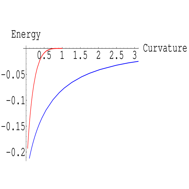
FIG. 1.: Bound state energy ($-\lambda_{n}^{2}$) vs curvature ($\kappa=1/R$): $n=0$ (blue line), $n=1$ (red line). The dependence of the energy as a function of the curvature is obtained through the solution of Eq. (29).

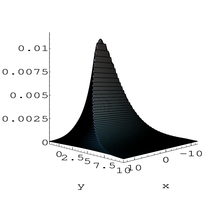
FIG. 2.: The wave function of the lowest bound state of the linear problem ($A=0$) is shown in the figure for $R=10$, $\nu=1$ (obtained through Eq. (34)).

In order to demonstrate that this linear bound state persists in the nonlinear limit we have performed full dynamical evolution simulations of Eq. (7), with an initial condition of the form expressed in Eq. (34), and demonstrated in Fig. 2. We note in passing that similar results have been obtained with other initial conditions such as e.g., a Thomas-Fermi initial profile of the form of Eq. (42). In particular, we show typical numerical simulation results in Fig. 3 for $R=10$, $\nu=A=1$. Notice that the $\delta$ function was represented as

$$\delta(s)=\sqrt{\frac{1}{\pi\epsilon}}\exp\left(-\frac{s^{2}}{2\epsilon}\right)$$ (53)

with $\epsilon=0.05$. The contour plot of Fig. 3 shows the result after a numerical evolution of 100 time units of Eq. (7).

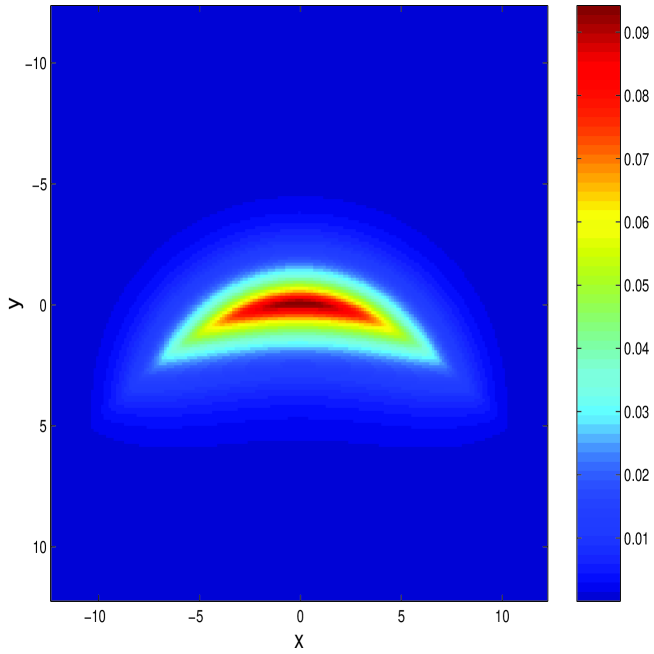
FIG. 3.: Contour plot of the solution of the partial differential equation of Eq. (7) with $f(x)=x^{2}/(2R)$, $R=10$, $\nu=A=1$ and initial condition given by the linear profile of Eq. (34).

The dynamical development indicates that after an initial transient the original linear profile slightly reshapes itself into the nonlinear solution depicted in Fig. 3. In the process, some radiation waves (“phonons”) are shed, that are absorbed by the absorbing boundary conditions used in a layer close to the the end of the domain (our computational box is of size $25\times 25$).

Beyond the proof-of-principle simulations for various initial conditions theoretically derived in sections III and IV, we also attempted to examine the dynamics of the nonlinear excitations of the channel. This was done using the following numerical protocol: after obtaining a quasi-relaxed nonlinear localized mode for the channel of the form $y=x^{2}/(2R)$, we moved the channel to a new position, namely $y=(x-1)^{2}/(2R)$. Notice that similar in spirit experiments have recently been carried in Bose-Einstein condensates [35], where the magnetic trap confining the condensate is displaced to a new position and the ensuing dynamics of the condensate are observed. The position of the center of mass of the initial condition profile was approximately obtained (using a trapezoidal approximation to the relevant two-dimensional integrals) as $(x(t=0),y(t=0))=(0.178,0.862)$. The new bottom of the channel (hence the point to which the center of mass should approach) in this case is $(x,y)=(1,0)$. In Fig. 4, the process of relaxation to this new equilibrium is shown as a function of time for a very long dynamical simulation of $t$ up to $1000$ time units. In this run, we observe (after an initial transient) a slow relaxation towards the new minimum of the potential well. Notice that despite the Hamiltonian nature of the model, the excitation of an “internal mode” of the nonlinear wave [36] can be dissipated due to mechanisms of coupling to extended wave, phonon modes, such as the ones reported in [37].

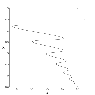
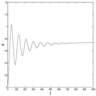
FIG. 4.: The top panel shows, for times between $t=500$ and $t=1000$, the time evolution of the center of mass in the $x-y$ plane (the motion proceeds from top left to bottom right as time evolves). The middle panel shows the time evolution of the $x$-position of the center of mass of the nonlinear excitation, while the bottom panel the slow evolution of the $y$-position of the center of mass.

VI Summary

In summary, we have shown that:

• In two-dimensional media with a curved infinitely thin waveguide (quantum channel) there exist bound states for linear and nonlinear self-interacting excitations;

• The finite curvature of the waveguide provides a stabilizing effect on otherwise unstable localized states of repelling excitations;

• The binding energy of both linear and nonlinear localized excitations decreases when the curvature of the waveguide increases.

• Such linear bound states as the ones found here persist in the nonlinear dynamical problem as localized excitations. These have been found to be robust for different initial conditions and are centered at the minimum (point of largest curvature) of the parabola. When, the mode is initialized away from this minimum, it slowly relaxes to it.

While our motivation was originally provided by the embedding of a waveguide in a two-dimensional photonic crystal (as well as from more general geometric considerations), interesting analogies have arisen through our investigation, that warrant further study. In particular, we note the analogy in the weakly nonlinear regime of the equation for the waveguide/quantum channel with that of the Bose-Einstein condensate behavior in the presence of a magnetic trap in atomic physics. Another topic worthy of further investigation is a more detailed numerical study of the stability of the nonlinear localized modes we have identified. Finally, another direction that could be of further interest is the examination of a case of a finite (rather than infinitesimal) width channel [which can be computational achieved e.g., by allowing the parameter $\epsilon$ of Eq. (53) to vary towards larger values]. The examination of thresholds for genuinely two-dimensional instabilities, such as e.g., the transverse or the snaking instability, would be of particular interest within the latter context.

Such studies are currently in progress and will be reported in future publications.

A

To find an expression for the Green’s function $G(u,u^{\prime};v,v^{\prime})$ we expand this function in terms of of the eigenfunctions of the equation

$$\frac{d^{2}F}{d\sigma^{2}}-\sigma^{2}\,F=-\mu F,$$ (A1)

under the boundary conditions

$$F\rightarrow 0,~{}~{}~{}~{}~{}u\rightarrow\pm\infty.$$ (A2)

Eq. (A1) under the boundary conditions (A2) has the solutions

$$F_{n}(u)=a_{n}\,e^{-\sigma^{2}/2}\,H_{n}\left(\sigma\right),~{}~{}~{}n=0,1,2,...$$ (A3)

($\sigma=u\,\sqrt{\lambda/R}$), which correspond to the eigenvalues

$$\mu=2n+1.$$ (A4)

Here $H_{n}\left(z\right)$ is the Hermite polynomial [30] and $a_{n}=\left(\lambda/R\pi\right)^{1/4}\,\left(2^{n}\,n!\right)^{-1/2}$ is the normalization constant. In terms of the functions (A3), the Green’s function has the form

$$G(u,u^{\prime};v,v^{\prime})=\sum_{n=0}^{\infty}F_{n}(u)\,F_{n}(u^{\prime})\,g_{n}(v,v^{\prime}).$$ (A5)

Inserting Eq. (A5) into Eq. (15) for the coefficients $g_{n}(v,v^{\prime})$ we obtain the equation

$$\frac{d^{2}g_{n}}{dv^{2}}-\frac{\lambda^{2}}{R^{2}}v^{2}\,g_{n}-\frac{\lambda}{R}(2n+1)\,g_{n}=\delta(v-v^{\prime}),$$ (A6)

under the condition

$$g_{n}\rightarrow 0,~{}~{}~{}~{}~{}v\rightarrow\infty.$$ (A7)

The line $v=0$, which is the $y>R/2$ of the ordinate axis, is used as the cut [38]. Following the usual machinery (see e.g. [38]), to avoid discontinuities in the solution along the cut we shall require that

$$\frac{dg_{n}}{dv}=0~{}~{}~{}at~{}~{}v=0~{}~{}~{}~{}~{}when~{}n=2m,$$ (A8)

$$g_{n}(0)=0~{}~{}~{}when~{}~{}n=2m+1~{}~{}(m=0,1,2,..).$$ (A9)

The solution of the equation (A6) with regard to the boundary conditions (A7) and (A9) has the form

$$g_{n}=\sqrt{\frac{\pi\,R}{4\lambda}}\,\{V(n+\frac{1}{2},v\,\sqrt{2\lambda/R})\,U(n+\frac{1}{2},v^{\prime}\,\sqrt{2\lambda/R})\,\theta(v^{\prime}-v)+$$ (A10)

$$U(n+\frac{1}{2},v\,\sqrt{2\lambda/R})\,V(n+\frac{1}{2},v\,\sqrt{2\lambda/R})\,\theta(v-v^{\prime})\}$$ (A11)

where $U(a,x)$ and $V(a,x)$ are the Weber parabolic cylinder functions [30] and $\theta(v)$ is the Heaviside step-function. Another equivalent representaion in terms of Whittaker functions [30] is

$$U(n+\frac{1}{2},x)=2^{-n/2-1/4}\,W\left(-\frac{n}{2}-\frac{1}{4},-\frac{1}{4},\frac{1}{2}\,x^{2}\right),$$ (A12)

$$V(n+\frac{1}{2},x)=\frac{2^{-n/2+3/4}\,n!}{\sqrt{\pi\,x}\,\Gamma(\frac{n}{2}+1)}\,M\left(-\frac{n}{2}-\frac{1}{4},\frac{1}{4},\frac{1}{2}\,x^{2}\right).$$ (A13)

REFERENCES

- [1] Nonlinear Science at the Dawn of the 21st Century, Eds P.L. Christiansen, M.P. Sørensen, A.C. Scott, Lecture Notes in Physics (Springer,Berlin, Heidelberg, New York,2000); Localization and Energy transfer in Nonlinear Systems, Eds L. Vázquez, R.S. Mackay, M.P.Zorzano (World Scientific, Singapore, 2003).
- [2] Photonic Crystals and Light Localization in the 21st Century, C. M. Soukoulis (ed.), NATO Science Series C563, (Kluwer Academic Dordrecht, Boston, London, 2001).
- [3] A. Mekis, J.C. Chen, I. Kurland, S. Fan, P.R. Villeneuve, and J.D. Joannopoulos, Phys. Rev. Lett. 77, 3787 (1996).
- [4] S. Noda, A. Alongkarn, and M. Imada, Nature (London), 407, 608 (2000).
- [5] Yu.S. Kivshar, P.G. Kevrekidis and S. Takeno, Phys. Lett. A, 307, 287 (2003).
- [6] B.J. van Wees, H. van Houten, C.W.J. Beenakker, J.G. Williamson, L.P. Kouwenhoven, D. van der Marel, and C.T. Foxon, Phys. Rev. Lett. 60, 848 (1988).
- [7] Nanostructure Physics and Fabrication, Eds M.A. Reed and W.P. Kirks, (Academic Press, New York,1989).
- [8] K. Ismail, S. Washburn, and K. Y. Lee, Appl. Phys. Lett. 59, 1998 (1991).
- [9] R. Pulwey, M. Rahm, J. Biberger, and D. Weiss, IEEE Transactions on magnetics 37, 2076 (2001).
- [10] T. Shinjo, T. Okuno, R. Hassdorf, K. Shigeto, and T. Ono, Science, 289, 930 (2000).
- [11] M. Klaui, C. A. F. Vaz, J. Rothman, J. A. C. Bland, W. Wernsdorfer, G. Faini, and E. Cambril, Phys. Rev. Lett. 90, 097202 (2003).
- [12] R.L. Schult, D.G. Ravenhall and H.W. Wyld, Phys. Rev. B39, 5476 (1989).
- [13] K.F. Berggren and Z.L. Ji, Phys. Rev. B43, 4760 (1991).
- [14] M. Andrews and C.M. Savage , Phys. Rev. A 50, 4535 (1994).
- [15] P. Exner and P. Seba, J. Math. Phys. 30, 2574 (1989).
- [16] J. Goldstone and R.L Jaffe, Phys. Rev. B 45,14100 (1992).
- [17] Yu. B. Gaididei and O.O. Vakhnenko, J. Phys.: Condens. Matter 6, 32229 (1994); O.O. Vakhnenko, Phys. Rev. B52, 17386 (1995).
- [18] P. Exner and T. Ichinose, J. Phys. A 34, 1439 (2001).
- [19] R.C.T. da Costa, Phys. Rev. A 23, 1982 (1981).
- [20] P.C. Schuster and R.L. Jaffe, e-print hep-th/0302216.
- [21] P. Exner and D. Krejcirik, J. Phys. A: Math. Gen. 34, 5969 (2001).
- [22] M. Encinosa and B. Etemadi, Phys. Rev. A 58, 77 (1998); M. Encinosa and L. Mott, Phys. Rev. A 68, 014102 (2003).
- [23] T. Harayama, P. Davis and K. S. Ikeda, Phys. Rev. Lett. 82, 3803 (1999).
- [24] A. Wallraff, A.V. Ustinov, V.V. Kurin, I.A. Shereshevsky, and N.K. Vdovicheva, Phys. Rev. Lett. 84, 151 (2000).
- [25] S.F. Mingaleev, Yu.S. Kivshar, and R.A. Sammut, Phys. Rev. E 62, 5777 (2000); S.F. Mingaleev and Yuri S. Kivshar Phys. Rev. Lett. 86, 5474 (2001).
- [26] Yu. B. Gaididei, S.F. Mingaleev and P.L. Christiansen, Phys. Rev. E 62 R53 (2000); J. Phys.:Condens. Matter 13,1 (2001).
- [27] A.E. Leanhardt, A.P. Chikkatur, D. Kielpinski, Y. Shin, T.L. Gustavson, W. Ketterle, and D.E. Pritchard, Phys. Rev. Lett. 89, 040401 (2002).
- [28] Encylopaedia of Mathematics, vol. 3 (Kluwer Academic Publishers, Dordrecht, Boston, London, 1989), p. 159.
- [29] D. Jones, Generalized Functions (McGraw-Hill Publishing Company, London 1966).
- [30] M. Abramowitz and I. Stegun, Handbook of Mathematical Functions (Dover Publications, Inc., New York, 1972).
- [31] see e.g., F. Dalfovo, S. Giorgini, L. P. Pitaevskii, and S. Stringari, Rev. Mod. Phys. 71, 463(1999).
- [32] Yu. B. Gaididei, P.L. Christiansen, K. Ø. Rasmussen, and M. Johansson, Phys. Rev. B 55 R13365 (1997).
- [33] V.M. Pérez-García, H. Michinel and H. Herrero, Phys. Rev. A 57, 3837 (1998); L. Salasnich, A. Parola and L. Reatto, Phys. Rev. A 65, 043614 (2002); Y.B. Band, I. Towers, and B.A. Malomed, Phys. Rev. A 67, 023602 (2003).
- [34] W.P. Reinhardt and C.W. Clark, J. Phys. B 30, L785 (1997); Th. Busch and J.R. Anglin, Phys. Rev. Lett. 84, 2298 (2000); D.J. Frantzeskakis et al., G. Theocharis, F.K. Diakonos, P. Schmelcher, and Yu.S. Kivshar, Phys. Rev. A 66, 053608 (2002); P. G. Kevrekidis, R. Carretero-González, G. Theocharis, D. J. Frantzeskakis, and B. A. Malomed, Phys. Rev. A 68, 035602 (2003).
- [35] A. Smerzi, A. Trombettoni, P.G. Kevrekidis and A.R. Bishop, Phys. Rev. Lett. 89, 170402 (2002); F.S. Cataliotti, L. Fallani, F. Ferlaino, C. Fort, P. Maddaloni and M. Inguscio, New. J. Phys. 5, 71 (2003).
- [36] Yu.S. Kivshar, D.E. Pelinovsky, Thierry Cretegny, and Michel Peyrard, Phys. Rev. Lett. 80, 5032 (1998); P.G. Kevrekidis and C.K.R.T. Jones, Phys. Rev. E 61, 3114 (2000).
- [37] M. Johansson and S. Aubry, Phys. Rev. E 61, 5864 (2000); P.G. Kevrekidis and M.I. Weinstein, Physica D 142, 113 (2000); P.G. Kevrekidis and M.I. Weinstein, Math. Comp. Simul. 62, 65 (2003).
- [38] P.M. Morse and H. Feshbach Methods of Theoretical Physics (McGraw-Hill Publishing Company, New York 1953).