Bubble generation in a twisted and bent DNA-like model

Abstract

The DNA molecule is modeled by a parabola embedded chain with long-range interactions between twisted base pair dipoles. A mechanism for bubble generation is presented and investigated in two different configurations. Using random normally distributed initial conditions to simulate thermal fluctuations, a relationship between bubble generation, twist and curvature is established. An analytical approach supports the numerical results.

I Introduction

In recent years, biomolecular modeling has received an ever increasing amount of attention, especially focused on the DNA molecule as well as protein structures. The basic structure of DNA is fairly well understood since the discovery of Crick and Watson Nat_171 , but it is becoming increasingly apparent that structure alone does not explain its complex functionality sufficiently Und DNA ; Saenger ; Yaku ; Reiss .

An example is the mechanism leading to bubble generation in DNA, in which the two polypeptide strands open to allow replication of the molecule, processing of proteins or complete strand separation (denaturation). Thermal fluctuations at physiological temperatures and nonlinear localizations are expected to produce bubbles when geometrical features, such as twist and curvature, are taken into account.

In initial works investigating the denaturation bubble, the geometrical features of the molecule were essentially neglected and energy localization was mostly attributed to inhomogeneities and impurities in the lattice chain, which may model the action of an enzyme PRA 40 ; PRE 53/1 ; PRE 67 ; PRE 55/4 ; JPA 35_10519 ; Muto ; PRE 49 , or nonlinear excitations PLA 154 ; Bang/Peyrard ; PRE 55/4 ; JBP 25 ; PRL 70 ; PRE 51 . Also, discreteness plays an important role for the localization of these excitations. The inhomogeneities have been modeled by different masses at various chain sites PRE 49 ; PRE 53/1 ; PRE 67 ; PRA 42 , by conformational defects PRE 51 or by changes in the coupling between molecular sites PRE 55/4 ; PRE 67 . Also, different on-site potentials JPA 35_10519 ; PRA 42 ; PRA 44 ; PNAS 100 have been used as inhomogeneities, corresponding to the different number of hydrogen bonds between the two strands. In DNA, the AT base pair connects through two hydrogen bonds, whereas the CG base pair has three. It has to some extent been experimentally verified that bubbles form at AT-rich sections of the DNA molecule PRL 90_138101 , but recent work NAR 32 also suggests that other mechanisms are involved.

Recently, both long-range dipole-dipole interaction PD 163 ; PLA 249 , helicity PLA 253 ; JBP 24 and curvature EPL 59 ; JPA 34_8465 ; Cond 13 have been included in the nonlinear transport theory, as well as combinations of these effects JPA 35_8885 ; PRE 66 ; JPA 34_6363 ; PRE 62 ; PLA 299 . It has been shown that chain geometry induces effects similar to those of impurities EPL 59 ; JPA 34_8465 ; JPA 35_8885 ; Cond 13 .

In biological environments, thermal fluctuations are always present and have been considered in Refs. PD 119 ; PRE 60 ; Muto ; PRE 47/1 ; PD 57 ; PRE 63_021901 , for example. In these references it was shown that solitons or discrete breathers can be generated from or exist among random thermal fluctuations.

The aim of the present work is to study an augmented Peyrard-Bishop model of the DNA molecule PRL 62 . We include both dipole-dipole long-range interaction and chain geometry in the form of a rigid, parabola embedded chain. Elaborating on earlier work Funnel , we show how both chain curvature and twist can initiate bubble generation in the DNA molecule. We consider two different chain configurations and randomly distributed initial conditions, modeling physiological temperatures.

In Sec. II, we introduce the model Hamiltonian and equations of motion and discuss relevant parameter values as well as the dipole interaction and chain geometry. In Sec. III, numerical investigations are performed and the results are supported by an analytical approach in Sec. IV. Finally, Sec. V contains a summary and a discussion.

II Model

We consider parabola embedded chains, as illustrated in Fig. 1. The base pair sites are embedded along a parabola in the $xy$ plane at uniform distances. The dipole moments of the base pairs, represented by arrows, are orthogonal to the parabola and twisted in the orthogonal plane. Within the $n$th base pair, the deviation from the equilibrium transverse distance between the bases is denoted $u_{n}$ PRL 62 .

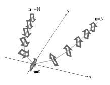
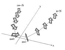
Figure 1: DNA chain embedded on a parabola in the $xy$ plane. Sites $(x_{n},y_{n})$ with $y_{n}=(\kappa/2)(x_{n}-\gamma)^{2}$, indicated by light grey dots. Base pair dipoles, orthogonal to the parabola, shown as dark grey arrows. Curvature $\kappa=2$ and twist $\tau=1$. The $z$ axis (not shown) forms a right-handed system with $x$ and $y$ axes. Left, the on-site case, $\gamma=0$. Right, the intersite case, $\gamma=1/2$.

The intrasite dynamics of the base pairs is governed by a Morse potential, see Fig. 2, and we assume a harmonic intersite coupling between neighboring base pairs. The coupling—or stacking—parameter, $C$, remains constant along the chain, i.e., independent of curvature and twisting.

As a result, using the scalings and parameter values presented below, we obtain the dimensionless Hamiltonian,

$$H = \sum_{n=-N}^{n=N}\left\{\frac{1}{2}\dot{u}_{n}^{2}+\frac{C}{2}\left(u_{n+1}-u_{n}\right)^{2}\right.$$ (1)

$$\quad+\left(e^{-u_{n}}-1\right)^{2}+\frac{1}{2}\displaystyle\left.\sum_{m}\right.^{\prime}J_{nm}u_{n}u_{m}\Big{\}},$$

where the prime indicates $m\neq n$ in the last summation, accounting for the long-range interaction (LRI) between the dipoles. The total number of sites are thus $N_{T}=2N+1$. Without the LRI, this Hamiltonian has previously been used to describe thermal denaturation in DNA, see Ref. PRE 47/1 .

Figure 2: The Morse potential $V_{\textrm{Morse}}(u_{n})=\left(e^{-u_{n}}-1\right)^{2}$ (solid curve). Effective potential, Eq. (9), in the analytical approximation (dashed curve).

The LRI is a dipole-dipole interaction, with coefficients $J_{nm}$ given by PD 163 ; Landau Lifshitz

$$J_{nm}=\frac{J\left\{{d}_{n}\cdot{d}_{m}-3\left({d}_{n}\cdot{r}_{nm}\right)\left({d}_{m}\cdot{r}_{nm}\right)\right\}}{|{r}_{n}-{r}_{m}|^{3}},$$ (2)

where ${r}_{n}$ and ${d}_{n}$ are the position vector and the unit dipole vector at the $n$th site, respectively, and ${r}_{nm}$ denotes the unit vector from the $n$th to the $m$th site

$${r}_{nm}=\frac{{r}_{n}-{r}_{m}}{|{r}_{n}-{r}_{m}|}.$$ (3)

We note that the geometry of the chain only comes into play through the LRI’s .

Dimensionless variables have been introduced as

$$u_{n}=\alpha\tilde{u}_{n},\quad t=\tilde{t}/t_{0},\quad{r}_{n}=\tilde{{r}}_{n}/l,\quad\textrm{ and }H=\tilde{H}/D,$$

where original physical variables are indicated by tildes. $l$ is the constant intersite distance between neighboring base pairs, $\alpha$ and $D$ are parameters in the dimensional Morse potential, $D\left(e^{-\alpha\tilde{u}_{n}}-1\right)^{2}$, and the time constant is given by $t_{0}=\sqrt{M/D\alpha^{2}}$, where $M$ is the mass of a base pair. The dimensionless parameters $C$ and $J$ are given by

$$C=\tilde{C}/(D\alpha^{2})\quad\textrm{ and }\quad J=2\tilde{J}_{0}/l^{3}D\alpha^{2},$$ (4)

with $\tilde{J}_{0}=q^{2}/4\pi\varepsilon_{0}$, where $q$ denotes the dipole charge of the base pair and $\varepsilon_{0}$ is the dielectric constant.

II.1 Parameter values

We use the parameter values $D=0.04$ eV ($=0.64\times 10^{-20}$ J), $\alpha=4.45\textrm{ \AA}^{-1}$ ($=4.45\times 10^{10}$ m^-1), $M=300\textrm{ a.m.u.}$ ($=5.00\times 10^{-25}$ kg) and the coupling parameter $\tilde{C}=0.06$ eV/$\textrm{\AA}^{2}$ ($=0.96$ J/m²), which have been widely used in DNA-like models PRE 47/1 ; PLA 299 ; PD 163 . The dimensionless stacking parameter then becomes $C=0.075$, which we use throughout the paper. We note that $\tilde{C}$-values between $0.003$ eV/$\textrm{\AA}^{2}$ PRL 62 and $31.7$ eV/$\textrm{\AA}^{2}$ PD 126 have been reported in the literature.

The resulting time constant, $t_{0}=0.20$ ps, is in the picosecond range, as seen in Table 1.

The dipole moment for the base pair, $d_{\textsf{dip}}$, is the geometric sum of the moments for the bases, which range between 3 and 7 debye JACS 113 . In our simulations we use $d_{\textsf{dip}}\approx 7$ debye. The corresponding dipole charge $q=d_{\textsf{dip}}/a_{\textsf{dip}}$, where $a_{\textsf{dip}}$ is the equilibrium distance between the dipole charges ($\approx 2$ ÅPD 163 ) then becomes $1.17\times 10^{-19}$ C, yielding $J=0.5$ .

Symbol	Parameter	Physical value
$\tilde{C}$	stacking	$0.96$ J/m2
$D$	Morse depth	$0.64\times 10^{-20}$ J
$\alpha$	inverse Morse width	$4.45\times 10^{10}$ m-1
M	base pair mass	$5.00\times 10^{-25}$ kg
$q$	dipole charge	$1.17\times 10^{-19}$ C
$\tilde{J}_{0}$	interaction strength	$0.90\times 10^{-28}$ Jm
$l$	lattice constant	$3.4\times 10^{-10}$ m
$t_{0}$	time constant	$0.20\times 10^{-12}$ s

Table 1: Physical parameters for the DNA molecule.

II.2 Geometry

We introduce the twist angle, $\phi_{n}$, which the dipoles create with the $z$ direction, in the form of a kink (5), where $\gamma$ gives the position of the kink center,

$$\phi_{n}=2\arctan\left[e^{-\tau\left(n-\gamma\right)}\right].$$ (5)

Thus, $\gamma$ is 0 in the on-site case, but $\gamma=1/2$ in the intersite case. The most important difference between the two is that the on-site case always has a dipole aligned in the bending plane at $n=0$ ($\phi_{0}=\pi/2$).

As illustrated in Fig. 3, the larger twist, $\tau$, the faster the twist angle changes — especially in the region of maximal twist and curvature. Note that the maximal slope of the twist function occurs at $\gamma$. In the limit $\tau\rightarrow\infty$, Eq. (5) gives $\phi_{n}=\pi$ for $n<0$, and $\phi=0$ for $n\geq 1$ for both cases. In the same limit, at $n=0$, the on-site case has $\phi_{0}=\pi/2$, whereas the inter-site case has $\phi_{0}=\pi$. In the limit $\tau\to 0$, all $\phi_{n}=\pi/2$ in both cases.

On the parabola embedded chain, $y_{n}=\left(\kappa/2\right)\left(x_{n}-\gamma\right)^{2}$, the resulting unit dipole vectors then become

$${d}_{n}=\big{(}-\xi_{n}\kappa\left(x_{n}-\gamma\right)\sin\phi_{n},\xi_{n}\sin\phi_{n},\cos\phi_{n}\big{)},$$ (6)

with $\xi_{n}=1/\sqrt{1+\kappa^{2}\left(x_{n}-\gamma\right)^{2}}$ (corresponding to the dark grey arrows in Fig. 1). In the on-site case, $x_{0}-\gamma\equiv 0$, and the other site positions are numerically calculated to fulfill the requirement that the distance between adjacent sites is always unity. In the intersite case, we define $x_{0}-\gamma\equiv-1/2$ and $x_{1}-\gamma\equiv 1/2$ and compute the other sites in a similar way. Thus, the axis of symmetry passes through the site $n=0$ in the on-site, $\gamma=0$, case and passes through the middle of the bond connecting sites $n=0$ and $n=1$ in the intersite, $\gamma=1/2$, case . See Fig. 1.

\psfrag{x1}[cc][cc]{$-\!10$}\psfrag{x2}[cc][cc]{$-\!5$}\psfrag{x3}[cc][cc]{$0$}\psfrag{x4}[cc][cc]{$5$}\psfrag{x5}[cc][cc]{$10$}\psfrag{y1}[cc][cc]{$0$}\psfrag{y2}[cc][cc]{$\frac{\pi}{2}$}\psfrag{y3}[cc][cc]{$\pi$}\psfrag{Site}[tt][tc]{Shifted site, $n-\gamma$}\psfrag{Twist}[Bc][Bc]{Twist angle, $\phi_{n}$}\includegraphics[width=170.71652pt]{PVL2_fig3.eps}

Figure 3: (Color online) The twist angle, $\phi_{n}$, for various values of the twist, $\tau$, around the chain center. On-site case, $\gamma=0$, intersite case, $\gamma=1/2$.

It is difficult to determine the actual value of the twist, $\tau$. The standard value for the twist angle between neighboring base pairs in an undisturbed DNA molecule is about $36^{\circ}$ PLA 253 ; JBP 24 ; PRE 66 . Requiring that a twist of $180^{\circ}$ should be achieved over five sites, thus corresponds to a value of $\tau$ about 1 (Fig. 3) in equilibrium and larger when twisted more.

Similarly, the bending of a DNA chain can be approximately determined from experimental results. In Refs. PLA 299 ; Cond 13 a parabolic approximation with curvature parameter $\kappa\leq 4$ was used. Here, we shall only consider the range $\kappa\leq 2$ as larger curvature has never been observed in measurements.

III Simulation results

From the Hamiltonian (1) we obtain the equations of motion

$$\ddot{u}_{n}+C\left(2u_{n}-u_{n-1}-u_{n+1}\right)$$

$$-2e^{-u_{n}}\left(e^{-u_{n}}-1\right)+\left.\sum_{m}\right.^{\prime}J_{nm}u_{m} = 0.$$ (7)

In the following we solve these equations numerically using a fourth order Runge-Kutta solver with free boundary conditions $u_{-N-1}=u_{-N}$ and $u_{N+1}=u_{N}$. In all simulations the relative change of the Hamiltonian is less than $10^{-5}$ and we consider a chain with $N_{T}=99$ sites.

In our previous work considering an approximate dipole-dipole interaction on a wedge shaped chain Funnel we investigated random initial conditions. This was done as nonlinear excitations are known to be generated from randomness Muto ; PD 57 ; PRE 47/1 ; PRE 60 ; PD 119 . As the outcome of collisions between nonlinear excitations depends strongly on their relative phases, we made 500 different random initial conditions to be able to find effects independent of the random phases. The random initial conditions created nonlinear excitations, which led to bubble generation at various collision sites. We found that bending of the chain caused the bubble generation to localize at the bent region.

In the following we use a similar approach to investigate the relationship between twist and curvature in this realistic expression for the dipole interaction (2). We consider random initial conditions: Initial displacements set to zero, i.e., $u_{n}(0)=0$ for all $n$, while initial velocities of the chain sites are normally distributed with mean value $\langle\dot{u}_{n}(0)\rangle=0$ and standard deviation $\sigma_{\dot{u}_{n}}$. The standard deviation is chosen to be $\sigma_{\dot{u}_{n}}=1.156$, corresponding a temperature of $T\approx 310$ K.

The system dynamics is simulated for 100 different realizations of the initial conditions with stepsize $0.01$ in time. The simulations run for 100 time units (corresponding to $20$ ps) or until the Hamiltonian is no longer conserved. As mentioned, the constant dipole-dipole interaction coefficient $J=0.5$ is used in all the simulations.

For different values of twist or curvature, the same initial condition can result in very different behavior. Consider Fig. 4, where the same initial condition is simulated for two different values of the twist, $\tau$, in the on-site case. With the larger twist (dashed curve) the amplitude grows in an exponential-like manner (see Sec. IV).

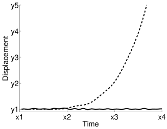
Figure 4: Evolution of the center site amplitude for $\kappa=1.0$ and $\tau=6$ (dashed curve) and $\tau=4$ (solid curve) for an on-site case.

At the end of each simulation, we examine the amplitudes. We use a threshold value of $u_{n}=100$, corresponding to about $20$ Å, i.e., twice the equilibrium distance between base pairs. If the threshold is exceeded in at least two adjacent sites, we consider this as a precursor for bubble generation. In the following sections, we have depicted the regions of curvature, $\kappa$, and twist, $\tau$, where at least one of the 100 simulations result in bubble generation.

III.1 Results for the on-site case

The combined effect of both curvature and twist for the on-site case is depicted in Fig. 5, where the shaded region corresponds to bubble generation. We see that bubbles are generated for strong twist and strong curvature, which is expected here. For the on-site case, the strongest attraction between dipoles occur at the sites $n=-1$ and $n=1$ (which are almost antiparallel for strong twist). Increasing the curvature bring these next-to-center sites closer, which augments the dipole-dipole interaction (2). As the inset (a) shows, the amplitude increase is localized to the region of maximal twist and curvature. We are aware that in reality, whole regions of DNA base pairs move apart during denaturation. Therefore, our mechanism should only be perceived as a precursor for bubble generation.

The exact shape of Fig. 5 depends on the chosen amplitude threshold—as well as system parameters—but its qualitative shape is unchanged. Close to the region border, only a few of the simultations results in bubble generation, but this number increases as one proceeds in the direction of stronger twist and larger curvature (i.e., towards the upper right corner). We note that for the on-site case the amplitude is increased at the three center sites $n=-1$, $n=0$, and $n=1$ as indicated in the inset (a).

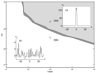
Figure 5: Region of bubble generation in the on-site case. Light grey region, bubble generation. Dark grey region, transition region indicating the uncertainty of the simulations. White region, no bubble generation. Insets show the displacement, $u_{n}$, versus site, $n$, at the points (a) and (b) at simulation times (a) $t=51$ and (b) $t=100$ for the same initial condition.

III.2 Results for the intersite case

In the intersite case, Fig. 6, the picture is different. First of all, the twist needed for bubble generation is smaller. Second, the dependence on the curvature is less pronounced. This is because the dipoles, that for strong twist are antiparallel, in this case are neighbors. Since, in the framework of our model, the chain has constant distance between adjacent sites, increasing the curvature does not increase the tendency for bubbles to be generated.

In fact, the opposite is the case: As the dipole twist is perpendicular to the chain, increasing the curvature has the consequence that the center dipoles interact in a less attracting way, since the center dipoles become more antiparallel (Fig. 8).

Note that in this case, the displacement at the two center cites, $n=0$ and $n=1$, is increased as the inset (a) shows. Close to the region border, the number of simulations resulting in bubble generation is small, but it increases as one increases the twist or decreases the curvature (i.e., moves to the upper left corner).

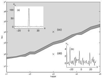
Figure 6: Region of bubble generation in the intersite case. Light grey region, bubble generation. Dark grey region, transition region indicating the uncertainty of the simulations. White region, no bubble generation. Insets show the displacement, $u_{n}$, versus site, $n$, at the points (a) and (b) at simulation time (a) $t=45$ and (b) $t=100$ for the same initial condition.

III.3 Effective potential

It is obvious that having initially randomly distributed energy along the chain, successful bubble generation should include, as a first stage, funneling of energy in the bent and twisted region. Therefore we can expect that only in the case when this region acts as a potential well, bubbling may occur. The behavior found in Figs. 5 and 6 can be qualitatively explained by the effective on-site potential, $V_{n}\equiv\sum_{m}^{\prime}J_{nm}$, which is introduced as

$$\sum_{n}\left.\sum_{m}\right.^{\prime}J_{nm}u_{n}u_{m} = -\frac{1}{2}\sum_{n}\left.\sum_{m}\right.^{\prime}J_{nm}\left(u_{n}-u_{m}\right)^{2}$$

$$\quad+\sum_{n}V_{n}u_{n}^{2}.$$

We consider the dipole potential at given sites for both the on-site and the intersite case for constant curvature, $\kappa=1.0$, with respect to the “ground state” at $n\to\pm\infty$. Thus, Fig. 7 depicts the depth of the potential well for constant curvature for both the on-site [Fig. 7(a)] and the intersite [Fig. 7(b)] case . We see that in the vicinity of the bending point, there exist an effective potential well for $\tau$ larger than about $0.5$. This corresponds to the behavior found in Figs. 5 and 6. The depth of the potential well increases with increasing twist, until a saturation is reached at $\tau\approx 5$. The existence of a potential well is a necessary, but not sufficient, condition for bubble generation.

    

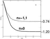
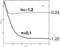
Figure 7: Effective potential $V_{n}-V_{\infty}$ for constant curvature $\kappa=1.0$. (a) On-site case. (b) Intersite case.

For constant twist, Fig. 8, we find different behaviors in the two chain configurations. For the on-site case with $\tau=6$ [Fig. 8(a)], we see a decreasing potential well depth with increasing curvature at sites $n=-1$ and $n=1$, whereas the potential at $n=0$ is almost constant. This corresponds to an effective potential well for increasing curvature in the on-site case. In the intersite case [Fig. 8(b)], the twist is fixed at $\tau=2$, but in contrast to the on-site case, we see that the depth of the potential well increases with increasing curvature at the center sites $n=0$ and $n=1$. Therefore, bubble generation is not found for larger curvature in the intersite case, corresponding to the behavior seen in Fig. 6.

    

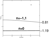
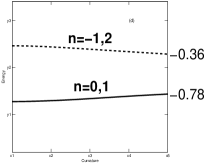
Figure 8: Effective potential $V_{n}-V_{\infty}$ for constant twist. (a) On-site case, $\tau=6$. (b) Intersite case, $\tau=2$.

Thus both curvature and twisting play a role in the localized formation of precursors for denaturation bubbles in our model of the DNA molecule and it is clear that the chain configuration is important. Stronger twist increases the initiation of bubble generation in both cases considered. The effect of increasing curvature is different: In the on-site case, curvature clearly enhances bubble generation, but in the intersite case it slightly decreases the formation of bubbles in the range of $\kappa$ considered.

Simulations for smaller values of the parameter $J$ showed that stronger twist was required to create bubbles.

IV Analytical approach

Considering only the center sites $n=0$ and $n=1$ in the intersite case, we are in effect looking at a dimer. Assuming that both displacements are equal, $u_{0}=u_{1}\equiv u$, the coupling term in the Hamiltonian, Eq. (1), vanishes and we are left with

$$H=\dot{u}^{2}+2\left(e^{-u}-1\right)^{2}-Ju^{2},$$ (8)

with $J=|J_{01}|=|J_{10}|$. For a strong twist, $\tau\gg 1$, the last term becomes negative, due to opposite dipole orientations, corresponding to attractive interaction. The effective potential

$$V(u)=2\left(e^{-u}-1\right)^{2}-Ju^{2}$$ (9)

is shown as the dashed curve in Fig. 2.

Equation (8) may now be integrated as

$$t-\bar{t}=\int_{\bar{u}}^{u}\frac{dw}{\sqrt{H-2\left(e^{-w}-1\right)^{2}+Jw^{2}}},$$ (10)

where $u=\bar{u}$ at the time $t=\bar{t}$. Choosing $\bar{t}$ so large that $w\gg 1$, the power term in the square root of Eq. (10), $Jw^{2}$, dominates (as seen in Fig. 2). Therefore, Eq. (10) may be approximated as

$$t-\bar{t}\approx\int_{\bar{u}}^{u}\frac{dw}{\sqrt{Jw^{2}}},$$

from which we find $u\varpropto\exp\left[\sqrt{J}(t-\bar{t})\right]$, in accordance with the exponential behavior found numerically in Fig. 4. A similar approach can be used for the on-site case with identical results.

V Conclusion

We have shown that bubble generation in DNA-like models can be initiated by curvature and twisting of the molecular strands.

Stronger twist facilitate bubble generation, whereas the effect of curvature depends on the details of the geometry. For the on-site case, increasing curvature increases the tendency for bubble generation. Conversely, the intersite case decreases bubble generation for increasing curvature.

Bubbles emerge in the region of maximal twist and curvature, and are found at physiological temperatures.

Numerical results are supported by analytical approximation. Widely used parameter values for DNA are used in our model.

- (1) J.D. Watson and F.H.C. Crick, Nature 171, 737 (1953).
- (2) C.R. Calladine and H.R. Drew, Understanding DNA (Academic, London, 2002).
- (3) W. Saenger, Principles of Nucleic Acid Structure (Springer-Verlag, New York, 1984).
- (4) L.V. Yakushevich, Nonlinear Physics of DNA (Wiley, New York, 1998).
- (5) C. Reiss, in Nonlinear Excitations in Biomolecules, edited by M. Peyrard (Springer, Les Ulis, 1994).
- (6) J.J.-L. Ting and M. Peyrard, Phys. Rev. E 53, 1011 (1996).
- (7) M. Techera, L.L. Daemen, and E.W. Prohofsky, Phys. Rev. A 40, 6636 (1989).
- (8) J. Cuevas, F. Palmero, J.F.R. Archilla, and F.R. Romero, J. Phys. A 35, 10519 (2002).
- (9) K. Forinash, T. Cretegny, and M. Peyrard, Phys. Rev. E 55, 4740 (1997).
- (10) V. Muto, A.C. Scott, and P.L. Christiansen, Phys. Lett. A 136, 33 (1989); Physica D 44, 75 (1990); V. Muto, Nanobiology 1, 325 (1992).
- (11) I. Bena, A. Saxena, G.P. Tsironis, M. Ibañes, and J.M. Sancho, Phys. Rev. E 67, 037601 (2003).
- (12) K. Forinash, M. Peyrard, and B. Malomed, Phys. Rev. E 49, 3400 (1994).
- (13) S.F. Mingaleev, P.L. Christiansen, Yu.B. Gaididei, M. Johansson, and K.Ø. Rasmussen, J. Biol. Phys. 25, 41 (1999).
- (14) O. Bang and M. Peyrard, Physica D 81, 9 (1995); Phys. Rev. E 53, 4143 (1996).
- (15) H. Feddersen, Phys. Lett. A 154, 391 (1991).
- (16) T. Dauxois and M. Peyrard, Phys. Rev. Lett. 70, 3935 (1993).
- (17) F. Zhang, M.A. Collins, and Yu.S. Kivshar, Phys. Rev. E 51, 3774 (1995).
- (18) M. Techera, L.L. Daemen, and E.W. Prohofsky, Phys. Rev. A 42, 1008 (1990).
- (19) M. Salerno, Phys. Rev. A 44, 5292 (1991).
- (20) T. Hwa, E. Marinari, K. Sneppen, and L.-h. Tang, Proc. Natl. Acad. Sci. U.S.A. 100, 4411 (2003).
- (21) G. Altan-Bonnet, A. Libchaber, and O. Krichevsky, Phys. Rev. Lett. 90, 138101 (2003).
- (22) C.H. Choi, G. Kalosakas, K.Ø. Rasmussen, M. Hiromura, A.R. Bishop and A. Usheva, Nucleic Acids Res. 32, 1584 (2004).
- (23) J. Cuevas, J.F.R. Archilla, Yu.B. Gaididei, and F.R. Romero, Physica D 163, 106 (2002).
- (24) L. Cruzeiro-Hansson, Phys. Lett. A 249, 465 (1998).
- (25) M. Barbi, S. Cocco, and M. Peyrard, Phys. Lett. A 253, 358 (1999).
- (26) M. Barbi, S. Cocco, M. Peyrard, and S. Ruffo, J. Biol. Phys. 24, 97 (1999).
- (27) P.L. Christiansen, Yu.B. Gaididei, and S.F. Mingaleev, J. Phys.: Condens. Matter 13, 1181 (2001).
- (28) S.F.M. Mingaleev, Yu.B. Gaididei, P.L. Christiansen, and Yu.S. Kivshar, Europhys. Lett. 59, 403 (2002).
- (29) R. Reigada, J.M. Sancho, M.I. Ibañes, and G.P. Tsironis, J. Phys. A 34, 8465 (2001).
- (30) J. Cuevas, F. Palmero, J.F.R. Archilla, and F.R. Romero, Phys. Lett. A 299, 221 (2002).
- (31) B. Sánchez-Rey, J.F.R. Archilla, F. Palmero, and F.R. Romero, Phys. Rev. E 66, 017601 (2002).
- (32) J.F.R. Archilla, Yu.B. Gaididei, P.L. Christiansen, and J. Cuevas, J. Phys. A 35, 8885 (2002).
- (33) J.F.R. Archilla, P.L. Christiansen, S.F. Mingaleev, and Yu.B. Gaididei, J. Phys. A 34, 6363 (2001).
- (34) Yu.B. Gaididei, S.F. Mingaleev, and P.L. Christiansen, Phys. Rev. E 62, R53 (2000).
- (35) A. Campa, Phys. Rev. E 63, 021901 (2001).
- (36) T. Dauxois, M. Peyrard, and A.R. Bishop, Phys. Rev. E 47, 684 (1993).
- (37) G.P. Tsironis, A.R. Bishop, A.V. Savin, and A.V. Zolotaryuk, Phys. Rev. E 60, 6610 (1999).
- (38) M. Peyrard, Physica D 119, 184 (1998).
- (39) T. Dauxois, M. Peyrard, and C.R. Willis, Physica D 57, 267 (1992).
- (40) M. Peyrard and A.R. Bishop, Phys. Rev. Lett. 62, 2755 (1989).
- (41) P.V. Larsen, P.L. Christiansen, O. Bang, J.F.R. Archilla, and Yu.B. Gaididei, Phys. Rev. E 69, 026603 (2004).
- (42) L.D. Landau and E.M. Lifshitz, The Classical Theory of Fields, revised 2nd ed. (Pergamon, Warsaw, 1962), p. 115.
- (43) M.V. Satarić, Physica D 126, 60 (1999).
- (44) J. Pranata, S.G. Wierschke, and W.L. Jorgensen, J. Am. Chem. Soc. 113, 2810 (1991).