A normal form of thin fluid film equations provides initial conditions

Abstract

We use dynamical systems theory to construct the normal form of the Navier–Stokes equations for the flow of a thin layer of fluid upon a solid substrate. The normal form equations illuminate the fluid dynamics by decoupling the long-term flow of interest from the rapid viscous decay of the transient shear modes. The normal form clearly shows the centre manifold of the lubrication model and shows the result that the initial condition for the fluid thickness of the lubrication model is not the initial physical fluid thickness, but instead is modified by the initial lateral shear flow. With these initial conditions, better forecasts will be made using the lubrication model. This dynamical systems approach will also enable similar illumination of other complicated models of dynamics.

1 Introduction

The flow of a thin layer of fluid is important in numerous industrial and natural processes: industrial applications include the coating processes of autobodies, beverage containers, sheet goods and films, decorative coating, and gravure roll coating; biomedical applications include the liquid films covering the cornea of the eye or protecting the linings of the lungs [5]. A variety of mathematical models of the fluid dynamics have been developed to aid understanding and prediction of the flow. For examples see the extensive reviews of Chang [2], Ruschak [15] or Oron, Davis and Bankoff [9]. On a flat substrate and in one lateral dimension the usual model for the evolution of a viscous fluid film’s thickness $\eta(x,t)$, driven only by surface tension, is the following nondimensional “lubrication” model [14, e.g.]

$${\frac{\partial\eta}{\partial t}}\approx-\mbox{$\frac{1}{3}$}\operatorname{We}{\frac{\partial}{\partial x}}\left(\eta^{3}{\frac{\partial^{3}\eta}{\partial x^{3}}}\right)\,,$$ (1)

where the Weber number $\operatorname{We}$ measures the strength of surface tension in the thin film flow. This is a considerable simplification of the governing equations when compared to the full Navier–Stokes equations.

Consider making a forecast with the lubrication model (1) from some initial state of the fluid, say with physical thickness $\eta_{0}$. Surely one just sets the initial field $\eta(x,0)$ to the initial thickness of the actual fluid $\eta_{0}(x)$. Herein we discover this is incorrect and that instead the correct initial condition for the lubrication model (1) is more accurately

$$\eta(x,0)\approx\eta_{0}-\operatorname{Re}{\frac{\partial}{\partial x}}\int_{0}^{\eta_{0}}(\eta_{0}y-{\textstyle\frac{1}{2}}y^{2})u_{0}\,dy\,,$$ (2)

where $u_{0}(x,y)$ is the initial lateral velocity field of the fluid, and $\operatorname{Re}$ is an appropriate Reynolds number. This initial condition accounts for the flow of fluid in the transient viscous decay of the initial velocity field.

For example, two colliding sheets of fluid form a hump. Suppose the initial fluid state is that of a constant thickness, $\eta_{0}$ constant, and Couette flow, $u_{0}=U_{0}f(x)y/\eta_{0}$ where $f(x)$ describes the lateral variations in strength of the initial lateral shear flow. Then from (2) the corresponding initial thickness for the model (1) is

$$\eta(x,0)\approx\eta_{0}-\operatorname{Re}\frac{5U_{0}\eta_{0}^{3}}{24}f^{\prime}(x)\,.$$ (3)

Two colliding sheets of fluids corresponds to a localised and negative derivative $f^{\prime}(x)$; in this case the initial condition (3) says the best forecast is obtained by starting the model from an initial condition with a hump proportional to $-f^{\prime}(x)$. This hump accounts for the transient collection of fluid at the collision as the lateral velocity decays through viscosity. This physically reasonable result agrees with earlier work [17, 16].

Here we develop analysis, Section 3.3, to determine that the parabolic weight function is correct in the integral of (2). Further, we introduce and use a framework, Section 3, to show that (2) is just the first approximation in an asymptotic series for the correct prescription of the initial conditions for the lubrication model (1), see Section 4. The theoretical framework is that of the normal form transformation in dynamical systems with centre manifolds [4, 3]. The continuity equation of incompressible fluid dynamics is an algebraic equation; thus, we make the novel application of the normal form transformation to differential algebraic systems.

Because of the complicated detail and form of the fluid dynamics equations, we introduce the normal form transformation in Section 2 using a relatively simple example dynamical system. The transformation is a near identity transformation with the aim of nonlinearly decoupling the dynamical equations as far as possible. In systems with a centre manifold, the centre manifold model appears immediately, see the example of Section 2.1, as first recognised by Elphick et al. [4]. Cox and Roberts [3] then recognised that the normal form also immediately provides the correct initial conditions for a model, see the example of Section 2.2. The example is a coupled differential algebraic system; in Sections 2.3–2.4 we show that the normal form may none-the-less be constructed in the usual manner.

Then in Section 3 we introduce the fluid equations and develop the normal form transformation that decouples the viscously decaying dynamics of lateral shear from the long lasting slow evolution of the thickness of the fluid film. When decoupled, the arguments of Section 4 provide initial conditions for the lubrication model (1). Equation (2) gives the leading nontrivial terms in the asymptotic expression for the initial condition.

2 An example introduces the normal form

Here we explore a straightforward artificial example (introduced in [16]) to illustrate the techniques used later in the normal form derivation of the initial conditions (2) for the lubrication model (1). This example reflects in detail many essential aspects of the relation between the normal form and initial conditions, and how to use the freedom inherent in the derivation. Someone very familiar with normal form transformations may skip this section.

Consider the following index $2$ differential-algebraic system which is structurally analogous to the thin fluid film equations (45–50) introduced in Section 3 (variable subscripts denote differentiation):

$$u_{t}+\epsilon u^{2}+uv+\epsilon p+\left(1+\epsilon^{2}\right)u+\epsilon\eta=0\,,$$ (4)

$$v_{t}+\epsilon uv+v^{2}+p+\left(1+\epsilon^{2}\right)v=0\,,$$ (5)

$$\quad\quad\epsilon u+v=0\,,$$ (6)

$$\eta_{t}+\epsilon u\eta-v=0\,.$$ (7)

Some trajectories of solutions are shown in Figure 1. In this section $u(t)$, $v(t)$, $p(t)$ and $\eta(t)$ represent analogues of a fluid film’s velocity, pressure and thickness. The small parameter $\epsilon$ is introduced to mimic slow lateral variations in the fluid thickness and flow. The normal form transformation we explore in this section clarifies the long term evolution of the above finite set of ordinary differential evolution equations.

$u$
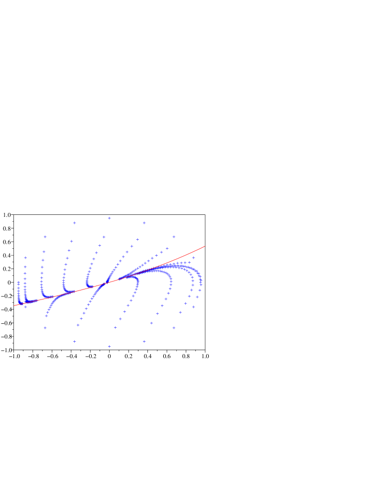
	$\eta$

Figure 1: simulations of the example system (4–7) for $\epsilon=0.4$ over time interval $6$ at time steps of $\Delta t=0.2$ and projected onto the $\eta u$-plane. This shows the exponential quick collapse of states onto the low-dimensional centre manifold (solid curve) given by (9).

Low-dimensional dynamics:

When $\epsilon=0$ , the system (4–7) has the equilibrium solutions $\eta=\mbox{const}$, $u=v=p=0$ (mimicking a uniform motionless fluid layer of thickness $\eta$). These equilibria, call the set of them ${\cal M}_{0}$, are stable: linearising, putting $\epsilon=0$ and seeking nontrivial solutions proportional to $\exp(\lambda t)$ leads to requiring the determinant

$$\left|\begin{array}[]{cccc}\lambda+1&0&0&0\\ 0&\lambda+1&0&0\\ 0&1&1&0\\ 0&-1&0&\lambda\end{array}\right|=\lambda(\lambda+1)=0\,.$$ (8)

This shows: the rapid ${\cal O}\big{(}e^{-t}\big{)}$ decay to any of the equilibria is determined by the $u$-equation (4); equation (7) determines $\eta$ is a neutral mode; whereas the other two equations do not contribute dynamics because of the need to satisfy the algebraic ‘continuity’ equation (6). For small $\epsilon\neq 0$ , instead of $\eta$ being constant, we thus expect that $\eta$ will evolve slowly on a nearby and similarly exponentially attractive set of states, called the centre manifold. This is confirmed by the numerical simulations shown in Figure 1. We soon, Section 2.1, confirm this nearby centre manifold of slow long term evolution is

$$u = -\epsilon\eta\left(1-3\epsilon^{2}\right)+\epsilon^{3}\eta^{2}+{\cal O}\big{(}\epsilon^{5}\big{)}\,,$$ (9)

$$v = \phantom{-}\epsilon^{2}\eta\left(1-3\epsilon^{2}\right)-\epsilon^{4}\eta^{2}+{\cal O}\big{(}\epsilon^{5}\big{)}\,,$$ (10)

$$p = -\epsilon^{2}\eta\left(1-\epsilon^{2}\right)+{\cal O}\big{(}\epsilon^{5}\big{)}\,.$$ (11)

On this centre manifold the slow model evolution is

$$\eta_{t}=\epsilon^{2}(1+\eta)\eta-\epsilon^{4}(1+\eta)(3+\eta)+{\cal O}\big{(}\epsilon^{5}\big{)}\,.$$ (12)

By the centre manifold relevance theorem [7, Chapt. 5, e.g.] or [1], we expect the long term behaviour of all nearby solutions are described by (9–12).

Elphick et al. [4] noted that low-dimensional centre manifold models such as (9–12) are an immediate consequence of transforming differential equations into a normal form. Cox & Roberts [3] observed that the projection of initial conditions onto such models also immediately follows from such a normal form. However, neither group explicitly addressed dynamics governed by systems of differential-algebraic equations. Here we demonstrate how the techniques adapt easily to differential-algebraic systems such as both (4–7) and also incompressible fluid dynamics, see Section 3. We illuminate the dynamics and modelling of such systems with a normal form transformation.

2.1 Interpret the normal form transformation

In Section 2.3 we will show how to construct the near identity transform to new dynamical variables that simplifies the description of the dynamics. But first we show how the resultant transformation illuminates the dynamics by decoupling the long-term evolution from the short-term decaying transients, and by decoupling the algebraic component of the governing equations. Substitute into the dynamical system (9–12), with new variables denoted by Fraktur font, the near identity transformation:

$$\eta = \mathfrak{h}+\epsilon(1+\mathfrak{h})\mathfrak{u}+\epsilon^{2}{\textstyle\frac{1}{2}}(1+\mathfrak{h})\mathfrak{u}^{2}+\epsilon^{3}(1+\mathfrak{h})[-(2+\mathfrak{h})\mathfrak{u}+\mbox{$\frac{1}{6}$}\mathfrak{u}^{3}]$$ (13)

$$\phantom{\mathfrak{h}}+\epsilon^{4}(1+\mathfrak{h})[-(\mbox{$\frac{7}{4}$}+\mbox{$\frac{3}{4}$}\mathfrak{h})\mathfrak{u}^{2}+\mbox{$\frac{1}{24}$}\mathfrak{u}^{4}]+{\cal O}\big{(}\epsilon^{5}\big{)}\,,$$

$$u = \mathfrak{u}-\epsilon\mathfrak{h}+\epsilon^{3}[(3+\mathfrak{h})\mathfrak{h}+{\textstyle\frac{1}{2}}(1+\mathfrak{h})\mathfrak{u}^{2}]+\epsilon^{4}\mbox{$\frac{1}{12}$}(1+\mathfrak{h})\mathfrak{u}^{3}+{\cal O}\big{(}\epsilon^{5}\big{)}\,,$$ (14)

$$v = \mathfrak{v}-\epsilon\mathfrak{u}+\epsilon^{2}\mathfrak{h}-\epsilon^{4}[(3+\mathfrak{h})\mathfrak{h}+{\textstyle\frac{1}{2}}(1+\mathfrak{h})\mathfrak{u}^{2}]+{\cal O}\big{(}\epsilon^{5}\big{)}\,,$$ (15)

$$p = \mathfrak{p}-\epsilon^{2}\mathfrak{h}-\epsilon^{3}(1+\mathfrak{h})\mathfrak{u}+\epsilon^{4}[\mathfrak{h}-{\textstyle\frac{1}{2}}(1+\mathfrak{h})\mathfrak{u}^{2}]+{\cal O}\big{(}\epsilon^{5}\big{)}\,.$$ (16)

Then the example dynamical system (4–7) becomes

$$\mathfrak{h}_{t}=\epsilon^{2}(1+\mathfrak{h})\mathfrak{h}-\epsilon^{4}(1+\mathfrak{h})(3+\mathfrak{h})+{\cal O}\big{(}\epsilon^{5}\big{)}\,,$$ (17)

$$\mathfrak{u}_{t}=-\left[\ 1+\epsilon^{2}(2+\mathfrak{h})-\epsilon^{4}(1+\mathfrak{h})(3+\mathfrak{h})\ \right]\mathfrak{u}+{\cal O}\big{(}\epsilon^{5}\big{)}\,,$$ (18)

$$\mathfrak{v}=\mathfrak{p}=0\,.$$ (19)

Crucially, the normal form system (17–19) captures all the solutions of the original system (4–7), at least in some neighbourhood of the equilibria ${\cal M}_{0}$. The reason is simply that the transformation (13–16) is a smooth reparametrisation of the complete state space near ${\cal M}_{0}$. Thus from arbitrary feasible initial conditions the normal form system (17–19) retains all the transient dynamics and all the long-term dynamics provided the dynamics stay within the neighbourhood of ${\cal M}_{0}$. Consider the effects of this transformation.

1. The algebraic part of the original system (4–7) is transformed into the trivial and decoupled algebraic equations (19), namely $\mathfrak{v}=\mathfrak{p}=0$ .

2. See immediately from the form (18) that $\mathfrak{u}=0$ is an invariant manifold of the dynamics, and is exponentially quickly attractive to a wide variety of nearby initial conditions. Thus this normal form clearly displays the attractive centre manifold is $\mathfrak{u}=0$ . In original variables, the transformation (13–16) then immediately shows the centre manifold maps to $\eta=\mathfrak{h}$ and the earlier claimed (9–11).

3. Also see the evolution (17) of $\mathfrak{h}$ reaffirms the earlier claimed centre manifold model (12).

4. Lastly, a crucial feature of the $\mathfrak{h}$ evolution (17) is that it is independent of $\mathfrak{u}$ in this normal form. Thus all states with the same $\mathfrak{h}$ but different $\mathfrak{u}$ only differ in the evolution of $\mathfrak{u}$, the $\mathfrak{h}$ evolution is identical. Next we use this to deal with initial conditions.

2.2 Project initial conditions

Consider the result of specifying some initial condition in a simulation, say

$$\eta(0)=\eta_{0}\,,\quad u(0)=u_{0}\,,\quad v(0)=v_{0}\,,\quad p(0)=p_{0}\,.$$ (20)

In general these will not lie on the centre manifold model (9–11), see for example the simulations shown in Figure 1. Following the arguments in [3], we use the normal form to deduce how to project such an initial condition into one for the low-dimensional model (12).

$u$
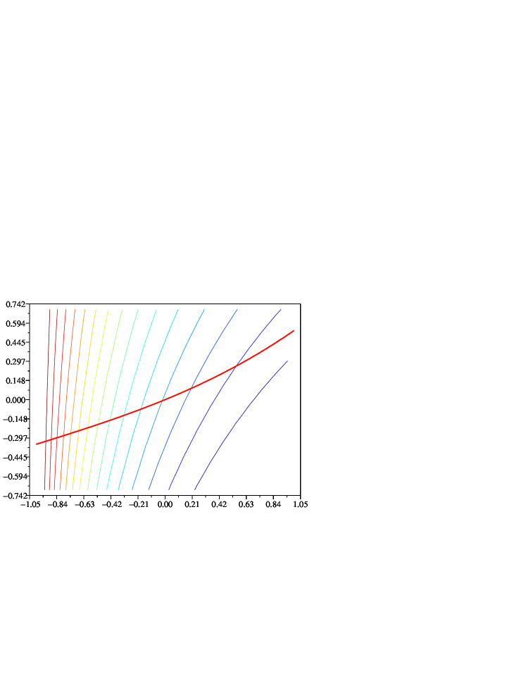
	$\eta$

Figure 2: centre manifold $\mathfrak{u}=0$ (thick curve) of the example system (4–7) for $\epsilon=0.4$ . The 16 transverse curves, called isochrons, show initial points which have the same long term dynamics.

But first we numerically illustrate the projection. Numerical solutions are feasible for simple systems. By running simulations, such as those in Figure 1, we draw contours of all initial conditions whose subsequent solutions end up at the same location (to an exponentially small difference) on the centre manifold after some fixed time, see Figure 2. All the points reaching the same location at the same fixed time must then have the same long term evolution. Hence, all initial conditions lying on one of the contours in Figure 2 must be projected onto the centre manifold where the contour intersects the manifold. Then the model will predict the correct long term evolution from the originally specified initial condition.

Any such initial condition corresponds to some point $(\mathfrak{h}_{0},\mathfrak{u}_{0},\mathfrak{v}_{0},\mathfrak{p}_{0})$ in the transformed variables. First, revert the series in the transformation (13–16) to find the initial state in the normal form variables

$$\mathfrak{h}_{0} = \eta_{0}-\epsilon(1+\eta_{0})u_{0}-\epsilon^{2}(1+\eta_{0})(\eta_{0}-{\textstyle\frac{1}{2}}u_{0}^{2})$$ (21)

$${}+\epsilon^{3}\mbox{$\frac{1}{6}$}(1+\eta_{0})(18+18\eta_{0}-u_{0}^{2})u_{0}$$

$${}+\epsilon^{4}\mbox{$\frac{1}{24}$}(1+\eta_{0})(84\eta_{0}^{2}+144\eta_{0}-90\eta_{0}u_{0}^{2}-102u_{0}^{2}+u_{0}^{4})+{\cal O}\big{(}\epsilon^{5}\big{)}\,,$$

$$\mathfrak{u}_{0} = u_{0}+\epsilon\eta_{0}-\epsilon^{2}(1+\eta_{0})u_{0}-\epsilon^{3}(4+2\eta_{0})\eta_{0}$$ (22)

$${}+\mbox{$\frac{1}{4}$}\epsilon^{4}(1+\eta_{0})(24+u_{0}^{2}+16\eta_{0})u_{0}+{\cal O}\big{(}\epsilon^{5}\big{)}\,,$$

$$\mathfrak{v}_{0} = v_{0}+\epsilon u_{0}\,,$$ (23)

$$\mathfrak{p}_{0} = p_{0}+\epsilon^{2}\eta_{0}-\epsilon^{4}\eta_{0}+{\cal O}\big{(}\epsilon^{5}\big{)}\,.$$ (24)

Second, for this system with an algebraic component the initial conditions (20) must be consistent with the algebraic constraints (19), namely $\mathfrak{v}_{0}=\mathfrak{p}_{0}=0$ ; hence, we require the original system to satisfy

$$v_{0}=-\epsilon u_{0}\quad\mbox{and}\quad p_{0}=-\epsilon^{2}\eta_{0}+\epsilon^{4}\eta_{0}+{\cal O}\big{(}\epsilon^{5}\big{)}\,.$$ (25)

Finally, when $\mathfrak{u}_{0}$ is non-zero the initial condition is off the centre manifold $\mathfrak{u}=0$ . But in the normal form (17–18) the evolution of $\mathfrak{h}$ is unaffected by the evolution of $\mathfrak{u}$. Further, $\mathfrak{u}$ decays to zero exponentially quickly. Thus, apart from an exponentially decaying transient, the evolution from $(\mathfrak{h}_{0},\mathfrak{u}_{0})$ will be identical to that from the point $(\mathfrak{h}_{0},0)$ on the centre manifold. Thus the appropriate initial condition for the low-dimensional model (12) is not $\eta(0)=\eta_{0}$ but instead that $\eta(0)=\mathfrak{h}_{0}$ as given by (21). This projection of the initial condition takes into account the initial transients in the dynamics.

2.3 Construct the normal form

We now explore how to construct the particular normal form transform (13–16) that has the requisite properties we used in the previous Section 2.2. The construction has considerable detail, see [3, 18, 8], with many subtleties in its application to this problem. To find the transformation (13–16) with corresponding evolution (17–19), we seek a near identity coordinate transform in the general form

$$\eta=\mathfrak{h}+{H}(\mathfrak{h},\mathfrak{u},\epsilon)\,,\quad u=\mathfrak{u}+{U}(\mathfrak{h},\mathfrak{u},\epsilon)\,,$$

$$v=\mathfrak{v}+{V}(\mathfrak{h},\mathfrak{u},\epsilon)\,,\quad p=\mathfrak{p}+{P}(\mathfrak{h},\mathfrak{u},\epsilon)\,,$$ (26)

such that the differential-algebraic system (4–7) takes this differential-algebraic normal form

$$\mathfrak{h}_{t}={\cal H}(\mathfrak{h},\epsilon)\,,\quad\mathfrak{u}_{t}=-\mathfrak{u}+{\cal U}(\mathfrak{h},\mathfrak{u},\epsilon)\,,\quad\mathfrak{v}=\mathfrak{p}=0\,,$$ (27)

where the functions ${H}$, ${U}$, ${V}$, ${P}$, ${\cal H}$ and ${\cal U}$ are strictly nonlinear functions of $\mathfrak{h}$, $\mathfrak{u}$ and $\epsilon$, and where we require

$${\cal U}\mbox{ strictly linear in }\mathfrak{u}\,,\quad\mbox{that is }{\cal U}\propto\mathfrak{u}\,.$$ (28)

That these properties (27–28) can be found is assured by the linearisation leading to (8): the zero eigenvalue assures that $\eta\approx\mathfrak{h}$ evolves nonlinearly; the $-1$ eigenvalue assures us that $u\approx\mathfrak{u}$ decays linearly with some nonlinear modifications; and the lack of other eigenvalues assures us that the normal form has two algebraic constraints on the other variables. The condition (28) ensures that $\mathfrak{u}=0$ , with $\mathfrak{v}=\mathfrak{p}=0$ , immediately describes the exponentially attractive centre manifold [4]. Consequently, the model evolution is simply $\mathfrak{h}_{t}={\cal H}(\mathfrak{h},\epsilon)$ , from (27), and the projection of initial conditions is done along curves of constant $\mathfrak{h}$.

The most straightforward construction uses iteration similar to that introduced for constructing centre manifolds [11]. Suppose we have some current approximation to the transformation and the evolution; for examples, $H=V=U=P={\cal H}={\cal U}=0$ is an initial approximation, whereas (13–18) is an approximation with errors ${\cal O}\big{(}\epsilon^{5}\big{)}$. Given some such approximation, we seek small corrections, denoted by primes, that improve the current approximation: that is, for example, we seek $u=\mathfrak{u}+U+U^{\prime}$ for some small $U^{\prime}$ to be determined. Substitute these into the governing system (4–7) and omit products of small corrections to obtain a system of equations to solve for corrections. For example, the left-hand side of the $\eta$-equation (7) becomes, upon using the chain rule,

$$\eta_{t}+\epsilon u\eta-v$$

$$= {\frac{\partial\eta}{\partial\mathfrak{h}}}{\frac{\partial\mathfrak{h}}{\partial t}}+{\frac{\partial\eta}{\partial\mathfrak{u}}}{\frac{\partial\mathfrak{u}}{\partial t}}+\epsilon u\eta-v$$

$$= \left(1+{\frac{\partial H}{\partial\mathfrak{h}}}+{\frac{\partial H^{\prime}}{\partial\mathfrak{h}}}\right)({\cal H}+{\cal H}^{\prime})+\left({\frac{\partial H}{\partial\mathfrak{u}}}+{\frac{\partial H^{\prime}}{\partial\mathfrak{u}}}\right)(-\mathfrak{u}+{\cal U}+{\cal U}^{\prime})$$

$${}+\epsilon(\mathfrak{u}+U+U^{\prime})(\mathfrak{h}+H+H^{\prime})-(\mathfrak{v}+V+V^{\prime})$$

$$\approx \left(1+{\frac{\partial H}{\partial\mathfrak{h}}}\right){\cal H}+{\frac{\partial H}{\partial\mathfrak{u}}}(-\mathfrak{u}+{\cal U})+\epsilon(\mathfrak{u}+U)(\mathfrak{h}+H)-(\mathfrak{v}+V)$$

$${}+{\cal H}^{\prime}-\mathfrak{u}{\frac{\partial H^{\prime}}{\partial\mathfrak{u}}}-V^{\prime}$$

$$= R_{\ref{sek}}+{\cal H}^{\prime}-\mathfrak{u}{\frac{\partial H^{\prime}}{\partial\mathfrak{u}}}-V^{\prime}\,,$$

where $R_{\ref{sek}}$ denotes the residual of (7) at the current approximation. Hence to choose corrections which reduce the residual we need to solve (32) below. Similarly for the other equations to require the solution of

$$\mathfrak{u}{\frac{\partial U^{\prime}}{\partial\mathfrak{u}}}-U^{\prime} = R_{\ref{seu}}+{\cal U}^{\prime}\,,$$ (29)

$$\mathfrak{u}{\frac{\partial V^{\prime}}{\partial\mathfrak{u}}}-V^{\prime}-P^{\prime} = R_{\ref{sev}}\,,$$ (30)

$$-V^{\prime} = R_{\ref{sec}}\,,$$ (31)

$$\mathfrak{u}{\frac{\partial H^{\prime}}{\partial\mathfrak{u}}}+V^{\prime} = R_{\ref{sek}}+{\cal H}^{\prime}\,,$$ (32)

where $R_{i}$ denotes the residual of the system’s equations (4–7) evaluated at the current approximation. For example, at the initial approximation $H=V=U=P={\cal H}={\cal U}=0$ , and using $\mathfrak{v}=\mathfrak{p}=0$ , the residuals

$$R_{\ref{seu}}=\epsilon\mathfrak{u}^{2}+\epsilon^{2}\mathfrak{u}+\epsilon\mathfrak{h}\,,\quad R_{\ref{sev}}=0\,,\quad R_{\ref{sec}}=\epsilon\mathfrak{u}\,,\quad\mbox{and}\quad R_{\ref{sek}}=\epsilon\mathfrak{u}\mathfrak{h}\,.$$ (33)

Now, see that the algebraic equation (6) immediately gives the $V$-correction through (31), and that the dynamic equation (5) for $v$ immediately gives the $P$-correction through (30). For example, in the initial iterate $V^{\prime}=-\epsilon\mathfrak{u}$ and $P^{\prime}=0$ . The other two components are more subtle.

• For equation (32), since $V^{\prime}$ is known, any term involving a factor $\mathfrak{u}^{q}$ in the residual $R_{\ref{sek}}-V^{\prime}$ will cause, via the homological operator $\mathfrak{u}{\frac{\partial H^{\prime}}{\partial\mathfrak{u}}}$, a term with $\mathfrak{u}^{q}/q$ in the transformation $H^{\prime}$; for example, with $R_{\ref{sek}}-V^{\prime}=\epsilon\mathfrak{u}(\mathfrak{h}+1)$ the correction $H^{\prime}=\epsilon\mathfrak{u}(\mathfrak{h}+1)$ . However, any term in the residual $R_{\ref{sek}}-V^{\prime}$ with no $\mathfrak{u}$ factor cannot be matched by a term in $H^{\prime}$, as $\mathfrak{u}{\frac{\partial H^{\prime}}{\partial\mathfrak{u}}}$ necessarily involves $\mathfrak{u}$, and must instead be matched by a term in the evolution ${\cal U}^{\prime}$. Thus the transformation is found so that the evolution of $\mathfrak{h}$ only involves $\mathfrak{h}$ itself as required by (27).

• For equation (29) any term involving a factor $\mathfrak{u}^{q}$ in the residual $R_{\ref{seu}}$ will cause, via the homological operator $\mathfrak{u}{\frac{\partial U^{\prime}}{\partial\mathfrak{u}}}-U^{\prime}$, a term with $\mathfrak{u}^{q}/(q-1)$ in the transformation $U^{\prime}$; for example, with $R_{\ref{seu}}=\epsilon\mathfrak{u}^{2}+\epsilon\mathfrak{h}$ the correction $U^{\prime}=\epsilon\mathfrak{u}^{2}-\epsilon\mathfrak{h}$ . However, any term linear in $\mathfrak{u}$, such as the term $\epsilon^{2}\mathfrak{u}$ in (33), must be used to correct the evolution via ${\cal U}^{\prime}$. Thus the transformation is done so that the evolution of $\mathfrak{u}$ satisfies (28).

In this manner iteration builds asymptotic approximations to the normal form transformation and the evolution, such as the earlier (13–19).

2.4 Homogeneous solutions provide freedom

There are extra complications because the normal form transformation is not unique. In general the transformations (26) are chosen to minimise the number of terms in the corresponding normal form dynamical equations (27) by placing as many terms as possible in the transformation (26). However, the result then depends upon our choice of basis for the algebra. Here we briefly explore the options available to us while retaining all the properties required to extract the centre manifold model and the projection of initial conditions.

As an aside note that the essential properties of the normal form are displayed in Figure 2: the curve of $\mathfrak{u}=0$ must correspond to the centre manifold (the thick curve); and the curves of constant $\mathfrak{h}$ must correspond to the isochrons (thin contours). Freedom comes from being able to parametrise these curves in state space in any smooth way consistent with these requirements.

The simplest way to identify freedom is to find the homogeneous solutions of the correction equations (29–32) for $H$, $V$, $U$, $P$, ${\cal H}$ and ${\cal U}$. The full homological operator [8, e.g.] for this problem appears on the left-hand side of (29–32); it operates on the space of multinomials in $\mathfrak{u}$, $\mathfrak{h}$ and $\epsilon$, but only the polynomials in $\mathfrak{u}$ are significant as $\mathfrak{h}$ and $\epsilon$ do not appear in the operator. First see that homogeneous solutions must have $V^{\prime}=P^{\prime}=0$ . Then, second, two families of linearly independent solutions are

$$(H^{\prime},{\cal H}^{\prime})=(\mathfrak{u}^{q},q\mathfrak{u}^{q})\,,\quad U^{\prime}={\cal U}^{\prime}=0\,,$$ (34)

and $$(U^{\prime},{\cal U}^{\prime})=(\mathfrak{u}^{q},(q-1)\mathfrak{u}^{q})\,,\quad H^{\prime}={\cal H}^{\prime}=0\,.$$ (35)

Thus we can always change an iterate by some linear combination of these solutions, multiplied by some function of $\mathfrak{h}$ and $\epsilon$, and only affect higher-order terms in the transformation.

• Consider (34) with $q\geq 1$ : introducing any such component will destroy the essential property that the evolution in $\mathfrak{h}$ is independent of $\mathfrak{u}$ that we require to use the normal form to project initial conditions. Thus we cannot use this freedom.

• Consider (34) with $q=0$ , that is $(H^{\prime},{\cal H}^{\prime})=(1,0)$ : introducing such a component, multiplied by an arbitrary function of $\mathfrak{h}$ and $\epsilon$, allows us to widely vary the relationship between the original variable $\eta$ and the transformed variable $\mathfrak{h}$. If we maintain the exact identity between these variables, $\eta=\mathfrak{h}$ when $\mathfrak{u}=0$ , then the model variable $\mathfrak{h}$ has the same physical meaning as the variable $\eta$. Although not essential, this seems desirable as it enhances physical interpretation. We choose this option.

  However, the normal form transformation may instead be used to immediately put the evolution equations on the centre manifold in one of the well established canonical normal forms [8, Chapt. 6], [10, Chapt. 3] or [7, Chapt. 3]. This alternative also uses the freedom identified here, but reduces the physical connection and is not implemented here.

• Consider (35) with $q=0$ , that is $(U^{\prime},{\cal U}^{\prime})=(1,-1)$ : we cannot use this freedom as, by introducing terms only in $\mathfrak{h}$ and $\epsilon$ into ${\cal U}^{\prime}$, it destroys the requirement that $\mathfrak{u}=0$ is the centre manifold of the $\mathfrak{u}$ evolution.

• Consider (35) with $q\geq 1$ : these homogeneous solutions allows us to alter the precise meaning of the transformed variable $\mathfrak{u}$ . Note that the linearised dynamics about the centre manifold $\mathfrak{u}=0$ are unaffected by any such change as terms linear in $\mathfrak{u}$, corresponding to $q=1$ , do not affect the evolution ${\cal U}^{\prime}$. For example, we could use this freedom to replace the strict linearity condition (28) for the evolution of $\mathfrak{u}$ and instead require the normal form

  $$u=\mathfrak{u}+U(\mathfrak{h},\epsilon)\,,\quad\mbox{and}\quad{\cal U}(\mathfrak{h},0,\epsilon)=0\,,$$ (36)

  so that $\mathfrak{u}$ measures precisely the departure of the state of the system from the centre manifold. For example, here the corresponding alternative normal form transform is

  $$\eta = \mathfrak{h}+\epsilon(1+\mathfrak{h})\mathfrak{u}+\epsilon^{2}{\textstyle\frac{1}{2}}(1+\mathfrak{h})\mathfrak{u}^{2}$$ (37)

  $$\phantom{\mathfrak{h}}-\epsilon^{3}\mbox{$\frac{1}{6}$}(1+\mathfrak{h})(12-\mathfrak{u}^{2}+6\mathfrak{h})\mathfrak{u}+{\cal O}\big{(}\epsilon^{4}\big{)}\,,$$

  $$u = \mathfrak{u}-\epsilon\mathfrak{h}+\epsilon^{3}(3+\mathfrak{h})\mathfrak{h}+{\cal O}\big{(}\epsilon^{4}\big{)}\,,$$ (38)

  $$v = \mathfrak{v}-\epsilon\mathfrak{u}+\epsilon^{2}\mathfrak{h}+{\cal O}\big{(}\epsilon^{4}\big{)}\,,$$ (39)

  $$p = \mathfrak{p}-\epsilon^{2}\mathfrak{h}-\epsilon^{3}(1+\mathfrak{h})\mathfrak{u}+{\cal O}\big{(}\epsilon^{4}\big{)}\,,$$ (40)

  with corresponding evolution

  $$\mathfrak{h}_{t}=\epsilon^{2}(1+\mathfrak{h})\mathfrak{h}+{\cal O}\big{(}\epsilon^{4}\big{)}\,,$$ (41)

  $$\mathfrak{u}_{t}=-[1+\epsilon^{2}(2+\mathfrak{h})]\mathfrak{u}-\epsilon^{3}{\textstyle\frac{1}{2}}(1+\mathfrak{h})\mathfrak{u}^{2}+{\cal O}\big{(}\epsilon^{4}\big{)}\,,$$ (42)

  $$\mathfrak{v}=\mathfrak{p}=0\,.$$ (43)

  We adopt this alternative when constructing the normal form of the dynamics of thin fluid films.

Using such freedom we find the centre manifold and the projection of initial conditions is the same. For example, the direction of the projection of initial conditions, the tangent to the isochrons [6, 3], at the centre manifold $\mathfrak{u}=0$ is the same, namely

$$\begin{bmatrix}\eta_{\mathfrak{u}}\\ u_{\mathfrak{u}}\\ v_{\mathfrak{u}}\\ p_{\mathfrak{u}}\end{bmatrix}=\begin{bmatrix}\epsilon(1+\mathfrak{h})-\epsilon^{3}(1+\mathfrak{h})(2+\mathfrak{h})\\ 1\\ -\epsilon\\ -\epsilon^{3}(1+\mathfrak{h})\end{bmatrix}+{\cal O}\big{(}\epsilon^{5}\big{)}\,.$$ (44)

This equivalence is reassuring because the different possible transformations still represent the same dynamical processes.

3 Normal form of thin fluid film equations

In this section we take the equations for a thin fluid film and transform them into a normal form that separates the dynamics of the viscously decaying modes from the large scale mode of slow evolution of the fluid film’s thickness.

3.1 Nondimensionalise the fluid film equations

Consider the two-dimensional flow of a thin film of Newtonian fluid along a flat substrate. We adopt a nondimensionalisation based upon the characteristic thickness of the film $H$, and some characteristic velocity $U$: for a specific example, in a regime where surface tension drives a flow against viscous drag the characteristic velocity is $U=\sigma/\mu$ and thus the Weber number $\operatorname{We}=\sigma/(U\mu)=1$ ; alternatively $U$ might be chosen to characterise the difference between a given initial lateral velocity and that corresponding to the lubrication model (1). Reverting to the general case, the reference length is $H$, the reference time $H/U$, and the reference pressure $\mu U/H$. The varying free surface is located at $y=\eta(x,t)$, where $x$ and $y$ are lateral and normal coordinates respectively. The flow, with velocity ${{\bf q}}=(u,v)$ and pressure $p$, is governed by the nondimensional incompressible Navier-Stokes equations

$$\operatorname{Re}({{\bf q}}_{t}+{{\bf q}}\cdot\nabla{{\bf q}}) = -\nabla p+\nabla^{2}{{\bf q}}\,,$$ (45)

where $\operatorname{Re}=UH\rho/\mu$ is a Reynolds number characterising the importance of the inertial terms compared to viscous dissipation, supplemented by the continuity equation

$$\nabla\cdot{{\bf q}} = 0\,,$$ (46)

non-slip boundary conditions on the substrate

$${{\bf q}}={\bf 0}\quad\mbox{on $y=0$\,,}$$ (47)

and tangential stress and normal stress conditions on the free surface

$$(1-\eta_{x}^{2})(u_{y}+v_{x})=2\eta_{x}(u_{x}-v_{y})\quad\mbox{on $y=\eta$\,,}$$ (48)

$$p+\frac{\operatorname{We}\eta_{xx}}{(1+\eta_{x}^{2})^{3/2}}=\frac{2}{1+\eta_{x}^{2}}\left[v_{y}+u_{x}-\eta_{x}(u_{y}+v_{x})\right]\quad\mbox{on $y=\eta$\,.}$$ (49)

We close the problem with the kinematic condition relating the velocity of the fluid on the surface to the evolution of the free surface:

$$\eta_{t}=-\partial_{x}\int_{0}^{\eta}u\,dy=v-u\eta_{x}\quad\mbox{on $y=\eta$\,.}$$ (50)

The fluid film is assumed to be so thin that the gravitational force in the momentum equations is neglected in this initial research project. The other main assumption we make is that the lateral variations are slow.

3.2 Introduce the normal form transform

Centre manifold techniques construct a model of the fluid flow assuming that lateral derivatives, $\partial_{x}$, are small [11, 12, e.g.]. Here we limit our aim to encompass flows with a lateral velocity which is also a small departure from the centre manifold of slow evolution. In the normal form we thus seek fields $\mathfrak{u}(x,y,t)$, $\mathfrak{v}(x,y,t)$, $\mathfrak{p}(x,y,t)$ and $\mathfrak{h}(x,t)$ which are a near identity transform of the physical fluid fields. We label these “quasi-” because they are approximately the same as the well known physical fields. Based upon the flow states we know for thin fluid films:

$$\eta=\mathfrak{h}+{\cal O}\big{(}\mathfrak{u}^{4/3}+\partial_{x}^{4}\big{)}\,,$$ (51)

$$v=\mathfrak{v}+{\cal O}\big{(}\mathfrak{u}^{4/3}+\partial_{x}^{4}\big{)}\,,$$ (52)

$$p=\mathfrak{p}-\operatorname{We}\mathfrak{h}_{xx}+{\cal O}\big{(}\mathfrak{u}^{4/3}+\partial_{x}^{4}\big{)}\,,$$ (53)

$$u=\mathfrak{u}+\operatorname{We}(\mathfrak{h}y-{\textstyle\frac{1}{2}}y^{2})\mathfrak{h}_{xxx}+{\cal O}\big{(}\partial_{x}^{5}\big{)}\,.$$ (54)

As in Section 2.4, see equation (36), we have here defined the lateral quasi-velocity $\mathfrak{u}$ to be exactly the lateral velocity field’s departure from that of the centre manifold model, approximately $\operatorname{We}(\mathfrak{h}y-{\textstyle\frac{1}{2}}y^{2})\mathfrak{h}_{xxx}$ . Because of the algebraic components in the fluid film equations we know the normal form has the two trivial algebraic equations

$$\mathfrak{v}=0\quad\mbox{and}\quad\mathfrak{p}=0\,.$$ (55)

Initially we assume the normal form also has trivial algebraic boundary conditions:

$$\mathfrak{u}=\mathfrak{v}=0\mbox{ on }y=0\,,\quad{\frac{\partial\mathfrak{u}}{\partial y}}=\mathfrak{p}=0\mbox{ on }y=\mathfrak{h}\,;$$ (56)

but later we find it is necessary to modify one of these. Lastly, the lateral quasi-velocity and the fluid quasi-thickness evolve according to

$${\frac{\partial\mathfrak{u}}{\partial t}} = {\cal U}(\mathfrak{u},\mathfrak{h})=\frac{1}{\operatorname{Re}}{\frac{\partial^{2}\mathfrak{u}}{\partial y^{2}}}+{\cal O}\big{(}\mathfrak{u}^{5/3}+\partial_{x}^{5}\big{)}\,,$$ (57)

$${\frac{\partial\mathfrak{h}}{\partial t}} = {\cal H}(\mathfrak{h})=-{\textstyle\frac{1}{3}}(\mathfrak{h}^{3}\mathfrak{h}_{xxx})_{x}+{\cal O}\big{(}\partial_{x}^{6}\big{)}\,,$$ (58)

where ${\cal U}(0,\mathfrak{h})=0$ . This last property of ${\cal U}$ ensures that the trivial $\mathfrak{u}=0$ forms the centre manifold of the dynamics. Hence (57) encapsulates that lateral shear flows dominantly decay by viscous diffusion, and the classic thin film model, $\mathfrak{h}_{t}\approx-{\textstyle\frac{1}{3}}(\mathfrak{h}^{3}\mathfrak{h}_{xxx})_{x}$ , is then recovered. This is our purpose for the normal form transformation (51–54).

Note that the very small difference, ${\cal O}\big{(}\mathfrak{u}^{4/3}+\partial_{x}^{4}\big{)}$, between the physical fluid thickness $\eta$ and the quasi-thickness $\mathfrak{h}$ identified in (51) means that evaluation on $y=\eta$ and $y=\mathfrak{h}$ are almost everywhere interchangeable to the order of accuracy determined in this section.

Also note that the form of many of the order of errors in the above are equivalent to having just one scaling parameter and assuming the lateral quasi-velocity field $|\mathfrak{u}|$ scales with $\partial_{x}^{3}$. However, here we are primarily interested in determining the dominant nontrivial effects of a lateral velocity field and thus we do not seek higher order in $\partial_{x}$ except where $\mathfrak{u}$ is involved. Consequently we later move to refine the approximations to a form where $|\mathfrak{u}|$ is asymptotically larger and scales with $\partial_{x}^{2}$—adopting a single scaling parameter would hinder this development so we adopt this more flexible expression of asymptotic errors.

In principle we proceed to use an iteration process to deduce the details of the normal form transformation. However, for the moment we only attempt just a little more than the first iteration. This is enough to discover highly nontrivial properties of the projection of initial conditions.

3.3 Fluid conservation evolves the free surface

Seek a correction to the free surface $\eta=\mathfrak{h}+\eta^{\prime}$ , using conservation of fluid (50):

$${\frac{\partial\eta}{\partial t}}=-\partial_{x}\int_{0}^{\eta}u\,dy$$ (59)

$$\Rightarrow {\frac{\partial\mathfrak{h}}{\partial t}}+{\frac{\partial\eta^{\prime}}{\partial t}}=-\partial_{x}\left[\int_{0}^{\eta}\mathfrak{u}\,dy+({\textstyle\frac{1}{2}}\mathfrak{h}\eta^{2}-\mbox{$\frac{1}{6}$}\eta^{3})\mathfrak{h}_{xxx}\right]+{\cal O}\big{(}\mathfrak{u}^{2}+\partial_{x}^{6}\big{)}$$

$$\Rightarrow {\frac{\partial\mathfrak{h}}{\partial t}}+{\frac{\partial\eta^{\prime}}{\partial t}}=-\partial_{x}\int_{0}^{\mathfrak{h}}\mathfrak{u}\,dy-{\textstyle\frac{1}{3}}(\mathfrak{h}\mathfrak{h}_{x}xx)_{x}+{\cal O}\big{(}\mathfrak{u}^{2}+\partial_{x}^{6}\big{)}$$

$$\Rightarrow {\frac{\partial\eta^{\prime}}{\partial t}}=-\partial_{x}\int_{0}^{\mathfrak{h}}\mathfrak{u}\,dy+{\cal O}\big{(}\mathfrak{u}^{2}+\partial_{x}^{6}\big{)}\,.$$

We used the known evolution of the film thickness (58), that $\mathfrak{h}_{t}\approx-{\textstyle\frac{1}{3}}(\mathfrak{h}^{3}\mathfrak{h}_{xxx})_{x}$ ; if we had not known this already, then at this step we would have discovered it was necessary; we can only put into $\eta^{\prime}$ terms which involve $\mathfrak{u}$ because terms which only involve $\mathfrak{h}$ are rendered ineffective in ${\frac{\partial\eta^{\prime}}{\partial t}}$ by the very slow evolution of $\mathfrak{h}$. Due to the form of the right-hand side for ${\frac{\partial\eta^{\prime}}{\partial t}}$ in (59), now try a change to the fluid thickness involving a weighted integral of the lateral velocity:

$$\eta^{\prime}=\partial_{x}\int_{0}^{\mathfrak{h}}w(y;\mathfrak{h})\mathfrak{u}\,dy+{\cal O}\big{(}\mathfrak{u}^{2}+\partial_{x}^{6}\big{)}$$

$$\Rightarrow {\frac{\partial\eta^{\prime}}{\partial t}}=\partial_{x}\Bigg{\{}\underbrace{{\frac{\partial\mathfrak{h}}{\partial t}}\mathfrak{u}(\mathfrak{h})w(\mathfrak{h};\mathfrak{h})}_{\text{negligible}}+\int_{0}^{\mathfrak{h}}w{\frac{\partial\mathfrak{u}}{\partial t}}+\underbrace{{\frac{\partial w}{\partial\mathfrak{h}}}{\frac{\partial\mathfrak{h}}{\partial t}}\mathfrak{u}}_{\text{negligible}}\,dy\Bigg{\}}+{\cal O}\big{(}\mathfrak{u}^{2}+\partial_{x}^{6}\big{)}$$

$$\Rightarrow {\frac{\partial\eta^{\prime}}{\partial t}}=\partial_{x}\left\{\int_{0}^{\mathfrak{h}}w\frac{1}{\operatorname{Re}}{\frac{\partial^{2}\mathfrak{u}}{\partial y^{2}}}\,dy\right\}+{\cal O}\big{(}\mathfrak{u}^{2}+\partial_{x}^{6}\big{)}$$

$$\Rightarrow {\frac{\partial\eta^{\prime}}{\partial t}}=\partial_{x}\left\{\frac{1}{\operatorname{Re}}\left[w{\frac{\partial\mathfrak{u}}{\partial y}}-w^{\prime}\mathfrak{u}\right]_{0}^{\mathfrak{h}}+\int_{0}^{\mathfrak{h}}w^{\prime\prime}(y)\frac{1}{\operatorname{Re}}\mathfrak{u}\,dy\right\}+{\cal O}\big{(}\mathfrak{u}^{2}+\partial_{x}^{6}\big{)}\,,$$

where primes on the weight function $w$ denote $y$ derivatives. Equate this to (59), recognising that $\mathfrak{u}=0$ on $y=0$ and ${\frac{\partial\mathfrak{u}}{\partial y}}=0$ on $y=\mathfrak{h}$ , to deduce the weight function satisfies

$$w^{\prime\prime}=-\operatorname{Re}\,,\quad w(0)=0\,,\quad w^{\prime}(\mathfrak{h})=0\quad\Rightarrow\quad w=\operatorname{Re}(\mathfrak{h}y-{\textstyle\frac{1}{2}}y^{2})\,.$$ (60)

Thus the free surface

$$\eta=\mathfrak{h}+\operatorname{Re}\partial_{x}\int_{0}^{\mathfrak{h}}(\mathfrak{h}y-{\textstyle\frac{1}{2}}y^{2})\mathfrak{u}\,dy+{\cal O}\big{(}\mathfrak{u}^{2}+\partial_{x}^{6}\big{)}\,,$$ (61)

in terms of the normal form fields $\mathfrak{h}$ and $\mathfrak{u}$.

Initial conditions:

Revert (61) and (54) to

$$\mathfrak{h}\approx\eta-\operatorname{Re}\partial_{x}\int_{0}^{\eta}(\eta y-{\textstyle\frac{1}{2}}y^{2})u\,dy\,,\quad\mbox{and}\quad\mathfrak{u}\approx u-(\eta y-{\textstyle\frac{1}{2}}y^{2})\eta_{xxx}\,.$$

Then recall that in the normal form (57–58), the quasi-velocity $\mathfrak{u}\to 0$ quickly through viscosity. Thereafter, when $\mathfrak{u}=0$ , the fluid thickness $\eta$ and the quasi-thickness $\mathfrak{h}$ are identical, by (61). Further, $\eta$ and $\mathfrak{h}$ evolve according to the same models, (1) and (58) respectively, and in the normal form (57–58) the evolution of the quasi-thickness $\mathfrak{h}$ is independent of quasi-velocity. Hence, from the above reversion, to make the correct long term forecast with the lubrication model we must start with the initial fluid thickness $\eta(x,0)$ as claimed in (2).

In the remainder of this section we demonstrate that this initial condition is the first nontrivial approximation in an asymptotic expansion based upon the normal form of thin film fluid dynamics.

3.4 Continuity updates the normal velocity

Upon substituting the current approximation, $u$ from (54) and $v\approx\mathfrak{v}+v^{\prime}$ where $\mathfrak{v}=0$ from (55), the continuity equation (46) implies

$$v=\mathfrak{v}-\int_{0}^{y}\mathfrak{u}_{x}\,dy-\partial_{x}[({\textstyle\frac{1}{2}}\mathfrak{h}y^{2}-\mbox{$\frac{1}{6}$}y^{3})\mathfrak{h}_{xxx}]+{\cal O}\big{(}\mathfrak{u}^{2}+\partial_{x}^{6}\big{)}\,.$$ (62)

As necessary, for quasi-fields $\mathfrak{v}=\mathfrak{u}=0$, this reduces to the well established normal velocity field for the centre manifold model.

3.5 Normal momentum updates pressure

Seek to update $p\approx\mathfrak{p}-\operatorname{We}\mathfrak{h}_{xx}+p^{\prime}$. Noting $u{\frac{\partial v}{\partial x}},v{\frac{\partial v}{\partial y}}={\cal O}\big{(}\mathfrak{u}_{x}^{2}+\partial_{x}^{8}\big{)}$ and ${\frac{\partial^{2}v}{\partial x^{2}}}={\cal O}\big{(}\mathfrak{u}^{2}+\partial_{x}^{6}\big{)}$ , consider

$$\operatorname{Re}\left[{\frac{\partial v}{\partial t}}+u{\frac{\partial v}{\partial x}}+v{\frac{\partial v}{\partial y}}\right]+{\frac{\partial p}{\partial y}}={\frac{\partial^{2}v}{\partial x^{2}}}+{\frac{\partial^{2}v}{\partial y^{2}}}$$

$$\Rightarrow -\mathfrak{u}_{xy}+\mathfrak{u}_{xy}^{0}+{\frac{\partial p^{\prime}}{\partial y}}=-\mathfrak{u}_{xy}-\operatorname{We}\partial_{x}[(\mathfrak{h}-y)\mathfrak{h}_{xxx}]+{\cal O}\big{(}\mathfrak{u}^{2}+\partial_{x}^{6}\big{)}$$

$$\Rightarrow p^{\prime}=\operatorname{We}\partial_{x}[{\textstyle\frac{1}{2}}(\mathfrak{h}-y)^{2}\mathfrak{h}_{xxx}]+(\mathfrak{h}-y)\mathfrak{u}_{xy}^{0}+p^{\prime\prime}+{\cal O}\big{(}\mathfrak{u}^{2}+\partial_{x}^{6}\big{)}\,,$$

where the superscript $0$ on $\mathfrak{u}_{xy}^{0}$ denotes evaluation on the substrate $y=0$ , soon the superscript $\mathfrak{h}$ will denote evaluation on the fluid surface $y=\mathfrak{h}$ , and $p^{\prime\prime}(x,t)$ is an integration constant to be determined from the free surface normal stress. The normal stress condition on $y=\eta$ is equivalent to evaluating on $y=\mathfrak{h}$ to as yet negligible relative error of ${\cal O}\big{(}\mathfrak{u}^{4/3}+\partial_{x}^{4}\big{)}$ ; thus

$$p(1+\eta_{x}^{2})+\operatorname{We}\eta_{xx}(1-{\textstyle\frac{1}{2}}\eta_{x}^{2})$$

$${}=2\left[{\frac{\partial v}{\partial y}}+\eta_{x}^{2}{\frac{\partial u}{\partial x}}-\eta_{x}\left({\frac{\partial u}{\partial y}}+{\frac{\partial v}{\partial x}}\right)\right]+{\cal O}\big{(}\mathfrak{u}^{2}+\partial_{x}^{6}\big{)}$$

$$\Rightarrow -\operatorname{We}(\mathfrak{h}_{xx}+\mathfrak{h}_{x}^{2}\mathfrak{h}_{xx})+p^{\prime\prime}+\operatorname{We}(\mathfrak{h}_{xx}-{\textstyle\frac{1}{2}}\mathfrak{h}_{x}^{2}\mathfrak{h}_{xx})$$

$${}=2\left[-\mathfrak{u}_{x}^{\mathfrak{h}}-{\textstyle\frac{1}{2}}\partial_{x}(\mathfrak{h}^{2}\mathfrak{h}_{xxx})+0-\mathfrak{h}_{x}\mathfrak{u}_{y}^{\mathfrak{h}}-0\right]+{\cal O}\big{(}\mathfrak{u}^{2}+\partial_{x}^{6}\big{)}$$

$$\Rightarrow p^{\prime\prime}=\operatorname{We}\partial_{x}(\mathfrak{h}^{2}\mathfrak{h}_{xxx})+\operatorname{We}\mbox{$\frac{3}{2}$}\mathfrak{h}_{x}^{2}\mathfrak{h}_{xx}-2\mathfrak{u}_{x}^{\mathfrak{h}}-2\mathfrak{u}_{y}^{\mathfrak{h}}\mathfrak{h}_{x}+{\cal O}\big{(}\mathfrak{u}^{2}+\partial_{x}^{6}\big{)}\,,$$

Hence the more refined description of the pressure field is

$$p = \mathfrak{p}-\operatorname{We}\left\{\mathfrak{h}_{xx}-\mbox{$\frac{3}{2}$}\mathfrak{h}_{x}^{2}\mathfrak{h}_{xx}+{\textstyle\frac{1}{2}}\partial_{x}[(\mathfrak{h}^{2}+2\mathfrak{h}y-y^{2})\mathfrak{h}_{xxx}]\right\}$$ (63)

$${}+(\mathfrak{h}-y)\mathfrak{u}_{xy}^{0}-2\partial_{x}(\mathfrak{u}^{\mathfrak{h}})+{\cal O}\big{(}\mathfrak{u}^{2}+\partial_{x}^{6}\big{)}\,.$$

3.6 Lateral momentum determines lateral velocity

Seek to update $u\approx\mathfrak{u}+u^{\prime}$ and ${\frac{\partial\mathfrak{u}}{\partial t}}\approx\frac{1}{\operatorname{Re}}{\frac{\partial^{2}\mathfrak{u}}{\partial y^{2}}}+{\cal U}^{\prime}$ . However, as flagged earlier, we are more interested in the effects of the lateral velocity field $\mathfrak{u}$ in the normal form rather than higher orders in the lateral gradients $\partial_{x}$ modifying the leading order evolution (58). Thus we change our expressions of errors to a form equivalent to scaling the lateral velocity $\mathfrak{u}$ with $\partial_{x}^{2}$ rather than with $\partial_{x}^{3}$ as done so far. Then working to errors ${\cal O}\big{(}\mathfrak{u}^{5/2}+\partial_{x}^{5}\big{)}$ enables us to resolve terms such as lateral diffusion $\mathfrak{u}_{xx}$ while omitting fifth derivatives of the free surface.

Using computer algebra, see [13] for the Reduce code, which also confirms that the residual in the Navier-Stokes equations (45) is ${\cal O}\big{(}\mathfrak{u}^{5/2}+\partial_{x}^{5}\big{)}$, we determine

$$\operatorname{Re}\left[{\frac{\partial u}{\partial t}}+u{\frac{\partial u}{\partial x}}+v{\frac{\partial u}{\partial y}}\right]+{\frac{\partial p}{\partial x}}={\frac{\partial^{2}u}{\partial x^{2}}}+{\frac{\partial^{2}u}{\partial y^{2}}}$$ (64)

$$\Rightarrow \operatorname{Re}{\cal U}^{\prime}+\operatorname{Re}{\frac{\partial u^{\prime}}{\partial t}}-{\frac{\partial^{2}u^{\prime}}{\partial y^{2}}}=\mathfrak{u}_{xx}-\partial_{x}[(\mathfrak{h}-y)\mathfrak{u}_{xy}^{0}]$$

$$\quad{}+2\mathfrak{u}_{xx}^{\mathfrak{h}}-2\mathfrak{h}_{x}^{2}\mathfrak{u}_{yy}^{\mathfrak{h}}+{\cal O}\big{(}\mathfrak{u}^{5/2}+\partial_{x}^{5}\big{)}\,,$$

At the free surface the tangential stress supplies

$$(1-\eta_{x}^{2})\left({\frac{\partial u}{\partial y}}+{\frac{\partial v}{\partial x}}\right)+2\eta_{x}\left({\frac{\partial v}{\partial y}}+{\frac{\partial u}{\partial x}}\right)=0$$ (65)

$$\Rightarrow {\frac{\partial u^{\prime}}{\partial y}}=\int_{0}^{\mathfrak{h}}\mathfrak{u}_{xx}\,dy+4\mathfrak{u}_{x}^{\mathfrak{h}}\mathfrak{h}_{x}+{\cal O}\big{(}\mathfrak{u}^{5/2}+\partial_{x}^{5}\big{)}\,,$$

when evaluated on the free surface, $y\approx\mathfrak{h}$ . We could satisfy this stress condition by changing the velocity field in the interior through a component in $u^{\prime}$. However, recall that the lateral quasi-velocity $\mathfrak{u}$ has more direct meaning when the normal form is chosen so that the physical velocity $u$ is independent of $\mathfrak{u}$ except for the leading term, see (54). Thus, satisfy this inhomogeneous bc by changing the surface boundary condition (56) for $\mathfrak{u}$ to

$${\frac{\partial\mathfrak{u}}{\partial y}}=\int_{0}^{\mathfrak{h}}\mathfrak{u}_{xx}\,dy+4\mathfrak{h}_{x}\mathfrak{u}_{x}^{\mathfrak{h}}+{\cal O}\big{(}\mathfrak{u}^{5/2}+\partial_{x}^{5}\big{)}\quad\mbox{on }y=\mathfrak{h}\,.$$ (66)

Consequently a new term on the left-hand side of (65) cancels the right-hand side terms, leaving the homogeneous bc ${\frac{\partial u^{\prime}}{\partial y}}=0$ on $y=\mathfrak{h}$ . Now consider the lateral momentum update equation (64): all terms in the right-hand side involve $\mathfrak{u}$ and so they are all placed into the evolution ${\cal U}^{\prime}$. Thus the lateral velocity is still given by (54), but we improve the description of the evolution to

$$\operatorname{Re}{\frac{\partial\mathfrak{u}}{\partial t}}=\mathfrak{u}_{yy}+\mathfrak{u}_{xx}-\partial_{x}[(\mathfrak{h}-y)\mathfrak{u}_{xy}^{0}]+2\mathfrak{u}_{xx}^{\mathfrak{h}}-2\mathfrak{h}_{x}^{2}\mathfrak{u}_{yy}^{\mathfrak{h}}+{\cal O}\big{(}\mathfrak{u}^{5/2}+\partial_{x}^{5}\big{)}\,.$$ (67)

As required, the normal form equation (67) with boundary condition (66) has $\mathfrak{u}=0$ as an attractive invariant (centre) manifold. Then with lateral quasi-velocity $\mathfrak{u}=0$ the lateral velocity field (54) reduces to the conventional thin fluid film approximation $u\approx\operatorname{We}(\mathfrak{h}y-{\textstyle\frac{1}{2}}y^{2})\mathfrak{h}_{xxx}$ .

3.7 Fluid conservation refines the evolution

We seek a further refinement to the description of the fluid thickness (61) using conservation of fluid (50). The aim is to discover more effects of the lateral velocity and so we work to errors ${\cal O}\big{(}\mathfrak{u}^{3}+\partial_{x}^{6}\big{)}$. There is considerable detail in determining the new terms, relegated to the computer algebra in [13], but the basic technique follows that used in Section 3.3. To the required order of accuracy we know the quasi-thickness evolution (58); thus the only freedom available is to update the fluid thickness from (61) by some small change $\eta^{\prime\prime}$. Substitute the lateral velocity field into (50) to obtain (using superscripts $0$ and $\mathfrak{h}$ to denote evaluation on the bed and quasi-surface, but now also using superscript $y$ to denote $\int_{0}^{y}\cdot\,dy$)

$${\frac{\partial\eta^{\prime\prime}}{\partial t}} = +\mbox{$\frac{1}{8}$}\mathfrak{h}^{4}\mathfrak{u}_{xxxy}^{0}+\mbox{$\frac{5}{6}$}\mathfrak{h}^{3}\mathfrak{h}_{x}\mathfrak{u}_{xxy}^{0}+\mbox{$\frac{1}{3}$}\mathfrak{h}^{3}\mathfrak{h}_{xx}\mathfrak{u}_{xy}^{0}+\mathfrak{h}^{2}\mathfrak{h}_{x}^{2}\mathfrak{u}_{xy}^{0}-\mbox{$\frac{2}{3}$}\mathfrak{h}^{3}\mathfrak{u}_{xxx}^{\mathfrak{h}}$$ (68)

$${}+2\mathfrak{h}^{3}\mathfrak{h}_{x}^{2}\mathfrak{u}_{xyy}^{\mathfrak{h}}+2\mathfrak{h}^{3}\mathfrak{h}_{x}\mathfrak{h}_{xx}\mathfrak{u}_{yy}^{\mathfrak{h}}-\mathfrak{h}^{2}(\mathfrak{u}_{xxx}^{y})^{\mathfrak{h}}-5\mathfrak{h}^{2}\mathfrak{h}_{x}\mathfrak{u}_{xx}^{\mathfrak{h}}-2\mathfrak{h}^{2}\mathfrak{h}_{xx}\mathfrak{u}_{x}^{\mathfrak{h}}$$

$${}+4\mathfrak{h}^{2}\mathfrak{h}_{x}^{3}\mathfrak{u}_{yy}^{\mathfrak{h}}-2\mathfrak{h}\mathfrak{h}_{x}(\mathfrak{u}_{xx}^{y})^{\mathfrak{h}}-4\mathfrak{h}\mathfrak{h}_{x}^{3}\mathfrak{u}_{x}^{\mathfrak{h}}+(\mathfrak{u}_{xxx}^{yyy})^{\mathfrak{h}}+\mathfrak{h}_{x}(\mathfrak{u}_{xx}^{yy})^{\mathfrak{h}}$$

$${}+{\cal O}\big{(}\mathfrak{u}^{3}+\partial_{x}^{6}\big{)}\,.$$

All these residual terms are ${\cal O}\big{(}u\partial_{x}^{3}\big{)}$, there is no component of ${\cal O}\big{(}u\partial_{x}^{2}\big{)}$. We summarise the details of the derivation in the next paragraph, but a solution for the above refinement of the fluid thickness $\eta$ is

$$\eta^{\prime\prime}(\mathfrak{h},\mathfrak{u}) = \operatorname{Re}\Big{\{}{\textstyle\int}_{0}^{\mathfrak{h}}(\mbox{$\frac{1}{24}$}y^{4}-\mbox{$\frac{1}{6}$}\mathfrak{h}y^{3}-\mbox{$\frac{1}{4}$}\mathfrak{h}^{2}y^{2}+\mbox{$\frac{3}{2}$}\mathfrak{h}^{3}y-\mbox{$\frac{1}{8}$}\mathfrak{h}^{4})\mathfrak{u}_{xxx}\,dy$$ (69)

$${}+\mathfrak{h}_{x}{\textstyle\int}_{0}^{\mathfrak{h}}(-\mbox{$\frac{1}{6}$}y^{3}-\mbox{$\frac{1}{2}$}\mathfrak{h}y^{2}+\mbox{$\frac{13}{2}$}\mathfrak{h}^{2}y-\mbox{$\frac{5}{6}$}\mathfrak{h}^{3})\mathfrak{u}_{xx}\,dy$$

$${}+\mathfrak{h}\mathfrak{h}_{x}^{2}{\textstyle\int}_{0}^{\mathfrak{h}}(4y-\mathfrak{h})\mathfrak{u}_{x}\,dy+\mathfrak{h}^{2}\mathfrak{h}_{xx}{\textstyle\int}_{0}^{\mathfrak{h}}(2y-\mbox{$\frac{1}{3}$}\mathfrak{h})\mathfrak{u}_{x}\,dy$$

$${}+12\mathfrak{h}^{3}\mathfrak{h}_{x}^{2}\mathfrak{u}_{x}^{\mathfrak{h}}+\mbox{$\frac{26}{3}$}\mathfrak{h}^{3}\mathfrak{h}_{x}\mathfrak{h}_{xx}\mathfrak{u}^{\mathfrak{h}}+7\mathfrak{h}^{2}\mathfrak{h}_{x}^{3}\mathfrak{u}^{\mathfrak{h}}+3\mathfrak{h}^{4}\mathfrak{h}_{x}\mathfrak{u}_{xx}^{\mathfrak{h}}$$

$${}+2\mathfrak{h}^{4}\mathfrak{h}_{xx}\mathfrak{u}_{x}^{\mathfrak{h}}+\mathfrak{h}^{4}\mathfrak{h}_{xxx}\mathfrak{u}^{\mathfrak{h}}-2\mathfrak{h}^{4}\mathfrak{h}_{x}^{3}\mathfrak{u}_{yy}^{\mathfrak{h}}\Big{\}}\,.$$

Thus for this $\eta^{\prime\prime}$ the normal form for the fluid thickness is now

$$\eta=\mathfrak{h}+\operatorname{Re}\partial_{x}{\textstyle\int}_{0}^{\mathfrak{h}}(\mathfrak{h}y-{\textstyle\frac{1}{2}}y^{2})\mathfrak{u}\,dy+\eta^{\prime\prime}(\mathfrak{h},\mathfrak{u})+{\cal O}\big{(}\mathfrak{u}^{3}+\partial_{x}^{6}\big{)}\,.$$ (70)

In the next section we use this transformation to determine more details about the initial conditions for the model of thin fluid film (1).

But before proceeding we overview the machinations needed to derive the refinement (69). Recall that the left-hand side ${\frac{\partial\eta^{\prime}}{\partial t}}$ is approximated by a formal expression:

$${\frac{\partial\eta^{\prime}}{\partial t}}\approx\frac{1}{\operatorname{Re}}{\frac{\partial\eta^{\prime}}{\partial\mathfrak{u}}}{\frac{\partial^{2}\mathfrak{u}}{\partial y^{2}}}\,.$$

Thus the components in the residual on the right-hand side of (68) which involve two or more derivatives of $y$ can be matched by a component in the refinement $\eta^{\prime\prime}$ with two less derivatives in $y$. The other components, involving the first $y$-derivative or integrals of the quasi-velocity $\mathfrak{u}$, must be matched by an integral component in the refinement $\eta^{\prime\prime}$ as we did in Section 3.3. I achieve such matching through considerable trial and error, and in three stages.

• Starting with the term with the most $y$-integrals, namely $(\mathfrak{u}_{xxx}^{yyy})^{\mathfrak{h}}$, the three $y$-derivatives in this boundary contribution is matched through multiple integration by parts of $\partial_{t}\mathfrak{u}_{xx}\propto\mathfrak{u}_{xxyy}$ with a weight function which is quartic in $y$. This and the bed component in $\mathfrak{h}^{4}\mathfrak{u}_{xxxy}^{0}$ gives the first integral in (69). This first term in (69) also changes some other terms in the residual (68). Then we progress to the other terms with less $y$-integrals and match them with simpler integrals as seen in (69).

• When all components as yet unmatched have two or more $y$-derivatives then we simply directly match them with the boundary contributions seen in (69).

• However, there is a difficulty: terms with odd $y$ derivatives and evaluated at the quasi-surface cannot be matched in the above procedure. Instead we use the surface boundary condition (66), either directly or its derivatives, to eliminate such terms. For example, differentiating (66) with respect to $x$ gives

  $$\mathfrak{u}_{xy}^{\mathfrak{h}}+\mathfrak{h}_{x}\mathfrak{u}_{yy}^{\mathfrak{h}}$$

  $$= {\textstyle\int}_{0}^{\mathfrak{h}}\mathfrak{u}_{xxx}\,dy+5\mathfrak{h}_{x}\mathfrak{u}_{xx}^{\mathfrak{h}}+4\mathfrak{h}_{xx}\mathfrak{u}_{x}^{\mathfrak{h}}+4\mathfrak{h}_{x}^{2}\mathfrak{u}_{xy}^{\mathfrak{h}}+{\cal O}\big{(}\mathfrak{u}^{5/2}+\partial_{x}^{5}\big{)}$$

  $$= {\textstyle\int}_{0}^{\mathfrak{h}}\mathfrak{u}_{xxx}\,dy+5\mathfrak{h}_{x}\mathfrak{u}_{xx}^{\mathfrak{h}}+4\mathfrak{h}_{xx}\mathfrak{u}_{x}^{\mathfrak{h}}-4\mathfrak{h}_{x}^{3}\mathfrak{u}_{yy}^{\mathfrak{h}}+{\cal O}\big{(}\mathfrak{u}^{5/2}+\partial_{x}^{5}\big{)}\,,$$

  where the last term $\mathfrak{u}_{xy}^{\mathfrak{h}}$ has a single $y$-derivative and so is replaced by its leading order approximation, namely $-\mathfrak{h}_{x}\mathfrak{u}_{yy}^{\mathfrak{h}}$. The above and higher order derivatives are implemented in computer algebra [13]. Similarly, time derivatives of (66), recalling $\operatorname{Re}\mathfrak{u}_{t}=\mathfrak{u}_{yy}$ , provide replacements for higher order odd $y$-derivatives of $\mathfrak{u}$.

With these methods we find that (69) is the solution for the update $\eta^{\prime\prime}$.

4 Revert the normal form to give initial conditions

Given an initial state of the fluid film we determine the appropriate initial condition for the fluid thickness in the lubrication model (1). First translate the initial condition to the normal form variables $\mathfrak{h}$ and $\mathfrak{u}$, then since the evolution of $\mathfrak{h}$ is independent of quasi-velocity $\mathfrak{u}$, the correct initial condition for the lubrication model (1) is $\eta(x,0)=\mathfrak{h}_{0}$ .

Suppose the fluid has initial thickness $\eta_{0}(x)$, lateral velocity field $u_{0}(x,y)$, normal velocity field $v_{0}(x,y)$ and pressure field $p_{0}(x,y)$. The fields $v_{0}$ and $p_{0}$ must be consistent with the fluid equations (45–50), but then play no role in the following. We revert (54) to obtain the initial quasi-lateral velocity

$$\mathfrak{u}_{0}=u_{0}-\operatorname{We}(\eta_{0}y-{\textstyle\frac{1}{2}}y^{2})\eta_{0xxx}+{\cal O}\big{(}\mathfrak{u}^{3}+\partial_{x}^{6}\big{)}\,,$$ (71)

as the quasi-thickness $\mathfrak{h}=\eta+{\cal O}\big{(}\mathfrak{u}^{3/2}+\partial_{x}^{3}\big{)}$, by (70) for example, and so $\mathfrak{h}$ is replaced by the initial fluid thickness $\eta_{0}$ to our order of accuracy. This quasi-lateral velocity $\mathfrak{u}_{0}$ characterises the distance from the initial fluid state to a state of the lubrication model.

Now find how this distance affects the initial fluid thickness. Revert (70) and evaluate at the initial fluid state, using (71) and $\mathfrak{h}=\eta+{\cal O}\big{(}\mathfrak{u}^{3/2}+\partial_{x}^{3}\big{)}$ , to give the initial quasi-thickness

$$\mathfrak{h}_{0}=\eta_{0}-\operatorname{Re}\partial_{x}\int_{0}^{\eta_{0}}(\eta_{0}y-{\textstyle\frac{1}{2}}y^{2})\mathfrak{u}_{0}\,dy-\eta^{\prime\prime}(\eta_{0},\mathfrak{u}_{0})+{\cal O}\big{(}\mathfrak{u}^{3}+\partial_{x}^{6}\big{)}\,,$$ (72)

where $\eta^{\prime\prime}$ is specified by (69). Recall the purpose of the normal form is to ensure the evolution of quasi-thickness $\mathfrak{h}$ is independent of the quasi-velocity and hence the transient viscous decay of lateral velocity will bring the fluid to the solution of the lubrication model (1) which started from the initial condition $\eta(x,0)=\mathfrak{h}_{0}$ as specified in (72). This initial condition permits us to make accurate long term forecasts with the model.

5 Conclusion

We use a normal form transformation to illuminate the dynamics of a thin layer of fluid. This is achieved by decoupling the slow long-lasting lubrication mode from the viscously decaying lateral shear modes. A simple example shows that the differential algebraic nature of the fluid equations is handled by straightforward modifications of the usual procedure to construct a normal form. Further, invoking the slowly-varying assumption that lateral derivatives are small enables us to deduce a normal form for the fluid dynamics albeit with significant technical detail requiring computer algebra to check. This normal form then provides us with the rationale to choose the initial condition (2) to make forecasts with the lubrication model(1). The next challenge is to connect this normal form analysis to the projection of initial conditions, started in [16], which is based upon the adjoint near a centre manifold model.

Acknowledgement:

I thank Sergey Suslov for his valuable input into all stages of this work.

References

• [1] J. Carr. Applications of centre manifold theory, volume 35 of Applied Math. Sci. Springer-Verlag, 1981.
• [2] H. C. Chang. Wave evolution on a falling film. Annu. Rev. Fluid Mech., 26:103–136, 1994.
• [3] S. M. Cox and A. J. Roberts. Initial conditions for models of dynamical systems. Physica D, 85:126–141, 1995.
• [4] C. Elphick, E. Tirapeugi, M. E. Brachet, P. Coullet, and G. Iooss. A simple global characterisation for normal forms of singular vector fields. Physica D, 29:95–127, 1987.
• [5] J. B. Grotberg. Pulmonary flow and transport phenomena. Annu. Rev. Fluid Mech., 26:529–571, 1994.
• [6] J. Guckenheimer. Isochrons and phaseless sets. J. Math. Biol., 1:259–273, 1975.
• [7] Y. A. Kuznetsov. Elements of applied bifurcation theory, volume 112 of Applied Mathematical Sciences. Springer-Verlag, 1995.
• [8] James Murdock. Normal forms and unfoldings for local dynamical systems. Springer Monographs in Mathematics. Springer, 2003.
• [9] A. Oron, S. H. Davis, and S. G. Bankoff. Long-scale evolution of thin liquid films. Rev. Mod. Phys., 69:931–980, 1997.
• [10] R. H. Rand and D. Armbruster. Perturbation methods, bifurcation theory and computer algebra, volume 65 of Applied Mathematical Sciences. Springer-Verlag, 1987.
• [11] A. J. Roberts. Low-dimensional modelling of dynamics via computer algebra. Computer Phys. Comm., 100:215–230, 1997.
• [12] A. J. Roberts. Low-dimensional modelling of dynamical systems applied to some dissipative fluid mechanics. In Rowena Ball and Nail Akhmediev, editors, Nonlinear dynamics from lasers to butterflies, volume 1 of Lecture Notes in Complex Systems, chapter 7, pages 257–313. World Scientific, 2003.
• [13] A. J. Roberts. Check the slowly-varying normal form of thin film fluids. Technical report, http://www.sci.usq.edu.au/staff/aroberts/nff.red, 2004.
• [14] R. Valery Roy, A. J. Roberts, and M. E. Simpson. A lubrication model of coating flows over a curved substrate in space. J. Fluid Mech., 454:235–261, 2002.
• [15] K. J. Ruschak. Coating flows. Annu. Rev. Fluid Mech., 17:65–89, 1985.
• [16] S. A. Suslov and A. J. Roberts. Proper initial conditions for the lubrication model of thin film fluid flow. Technical report, http://arXiv.org/abs/chao-dyn/9804018, 1998.
• [17] S. A. Suslov and A. J. Roberts. Projection of initial conditions for thin film flow models. In IUTAM Symposium on Nonlinear Wave Behavior in Multi-Phase Flow, 1999.
• [18] L. Vallier. An algorithm for the computation of normal forms and invariant manifolds. In Proceedings of the 1993 international symposium on Symbolic and algebraic computation table of contents, pages 225–233, 1993.