Anomalous scaling of a passive scalar advected by the Navier–Stokes velocity field: Two-loop approximation

Abstract

The field theoretic renormalization group and operator product expansion are applied to the model of a passive scalar quantity advected by a non-Gaussian velocity field with finite correlation time. The velocity is governed by the Navier–Stokes equation, subject to an external random stirring force with the correlation function $\propto\delta(t-t^{\prime})k^{4-d-2\varepsilon}$. It is shown that the scalar field is intermittent already for small $\varepsilon$, its structure functions display anomalous scaling behavior, and the corresponding exponents can be systematically calculated as series in $\varepsilon$. The practical calculation is accomplished to order $\varepsilon^{2}$ (two-loop approximation), including anisotropic sectors. Like for the well-known Kraichnan’s rapid-change model, the anomalous scaling results from the existence in the model of composite fields (operators) with negative scaling dimensions, identified with the anomalous exponents. Thus the mechanism of the origin of anomalous scaling appears similar for the Gaussian model with zero correlation time and non-Gaussian model with finite correlation time. It should be emphasized that, in contrast to Gaussian velocity ensembles with finite correlation time, the model and the perturbation theory discussed here are manifestly Galilean covariant. The relevance of these results for the real passive advection, comparison with the Gaussian models and experiments are briefly discussed.

I Introduction

In recent years, considerable progress has been achieved in the understanding of intermittency and anomalous scaling of fluid turbulence. Both the natural and numerical experiments suggest that the deviation from the classical Kolmogorov theory [1, 2, 3] is even more strongly pronounced for a passively advected scalar field $\theta(x)\equiv\theta(t,{\bf x})$ (temperature, entropy, density of an impurity etc) than for the velocity field itself; see e.g. Ref. [3, 4, 5, 6] and literature cited therein. At the same time, the problem of passive advection appears more easily tractable theoretically: even simplified models describing the advection by a “synthetic” velocity field ${\bf v}(x)\equiv\{v_{i}(x)\}$ with a given Gaussian statistics reproduce many of the anomalous features of genuine turbulent heat or mass transport observed in experiments. Therefore, the problem of passive scalar advection, being of practical importance in itself, may also be viewed as a starting point in studying intermittency and anomalous scaling in the turbulence on the whole.

The issue of interest is, in particular, the behavior of the equal-time structure functions of the scalar field

$$S_{n}(r)=\big{\langle}[\theta(t,{\bf x})-\theta(t,{\bf x^{\prime}})]^{n}\big{\rangle},\qquad{\bf r}={\bf x}-{\bf x^{\prime}},\quad r=|{\bf r}|.$$ (1)

The concept of anomalous scaling implies a power-law behavior of the functions (1) in the inertial-convective range of scales, $S_{n}\propto r^{\zeta_{n}}$, with a nonlinear dependence of the exponents $\zeta_{n}$ on $n$; see e.g. Refs. [1, 2, 3, 4, 5, 6].

The crucial breakthrough in theoretical research is related to a simple model of a passive scalar quantity advected by a random Gaussian field, white in time and self-similar in space, known as the Kraichnan’s rapid-change model [7]. There, for the first time the existence of anomalous scaling was established on the basis of a microscopic model [8] and the corresponding anomalous exponents were calculated within controlled approximations [9, 10, 11, 12] and a systematic perturbation expansion in a formal small parameter [13]. Detailed review of the recent theoretical research on the passive scalar problem and the bibliography can be found in Ref. [14].

In the “zero-mode approach,” developed in [9, 10, 11, 12] (see also [14]), nontrivial anomalous exponents are related to the zero modes (unforced solutions) of the closed exact differential equations satisfied by the equal-time correlation functions. From the field theoretic viewpoint, this is a realization of the well-known idea of self-consistent (bootstrap) equations, which involve skeleton diagrams with dressed lines and dropped bare terms. Owing to very special features of the rapid-change models (linearity in the passive field and time decorrelation of the advecting field) such equations are exactly given by one-loop approximations, and the resulting equations in the coordinate space are differential (and not integral or integro-differential as in the case of a general field theory). In this sense, the model is “exactly solvable.” Furthermore, in contrast to the case of nonzero correlation time, closed equations are obtained for the equal-time correlations, which are Galilean invariant and, therefore, not affected by the so-called “sweeping effects” that would obscure the relevant physical interactions.

The second systematic analytical approach to the rapid-change model, proposed in papers [13], is based on the field theoretic renormalization group (RG) and operator product expansion (OPE). There, anomalous scaling emerges as a consequence of the existence in the model of composite fields with negative scaling dimensions (“dangerous composite operators”), identified with the anomalous exponents. This allows one to give alternative derivation of the anomalous scaling, to construct a systematic perturbation expansion for the anomalous exponents, analogous to the famous $\varepsilon$ expansion in the RG theory of critical behavior (see the monographs [15, 16] and references therein), and to calculate the exponents to the second [13, 17] and third [18, 19] orders.

The two approaches complement each other well: the zero-mode technique allows for exact (nonperturbative) solutions for the anomalous exponents related to second-order correlation functions [10, 20, 21] (they are nontrivial for passive vector fields or anisotropic sectors for scalar fields), while the RG approach form the basis for systematic perturbative calculations of the higher-order anomalous exponents. For anisotropic velocity ensembles or/and passively advected vector fields, as well as for passive advection of extended objects (polymers or membranes), where the calculations become rather involved, all the existing results for higher-order correlation functions were derived only by means of the RG approach and only to the leading order in $\varepsilon$ [22, 23, 24, 25].

From a more physical point of view, zero modes can be interpreted as statistical conservation laws in the dynamics of particle clusters [26]. The concept of statistical conservation laws appears rather general, being also confirmed by numerical simulations of Refs. [27, 28], where the passive advection in the two-dimensional Navier–Stokes (NS) velocity field [27] and a shell model of a passive scalar [28] were studied. This observation is rather intriguing because in those models no closed equations for equal-time quantities can be derived due to the fact that the advecting velocity has a finite correlation time (for a passive field advected by a velocity with given statistics, closed equations can be derived only for different-time correlation functions, and they involve infinite diagrammatic series).

One may thus conclude that breaking the artificial assumptions of the time decorrelation and Gaussianity of the velocity field is the crucial point.

Besides the calculational efficiency, an important advantage of the RG approach is its relative universality: it is not bound to the aforementioned “solvability” of the rapid-change model and can also be applied to the case of finite correlation time or non-Gaussian advecting field. In Refs. [29, 30] (see also [31] for the case of compressible flow and [32] for a passive vector field) the RG and OPE were applied to the problem of a passive scalar advected by a Gaussian self-similar velocity with finite (and not small) correlation time. The energy spectrum of the velocity in the inertial range has the form ${\cal E}(k)\propto k^{1-2\varepsilon}$, while the correlation time at the momentum $k$ scales as $t(k)\propto k^{-2+\eta}$. It was shown that, depending on the values of the exponents $\varepsilon$ and $\eta$, the model reveals various types of inertial-range scaling regimes with nontrivial anomalous exponents, which were explicitly derived to the first [29, 31] and second [30] orders of the double expansion in $\varepsilon$ and $\eta$. The most interesting case is $\eta=\varepsilon$, when the exponents can be nonuniversal through the dependence on the ratio of the velocity correlation time and the turnover time of the passive scalar.

Earlier, a similar model was proposed and studied in detail (using numerical simulations, in two dimensions) in [33]. Various aspects of the transport and dispersion of particles in random Gaussian self-similar velocity fields with finite correlation time were also studied in Refs. [34, 35, 36, 37, 38, 39, 40, 41].

As was pointed out in Ref. [33], the Gaussian model with finite correlation time suffers from the lack of Galilean invariance and therefore misrepresents the self-advection of turbulent eddies. It is well known that the different-time correlations of the Eulerian velocity field are not self-similar, as a result of these “sweeping effects,” and depend substantially on the integral scale. It would be much more appropriate to impose the scaling relations for ${\cal E}(k)$ and $t(k)$ in the Lagrangian frame, but this is embarrassing due to the daunting task of relating Eulerian and Lagrangian statistics for a flow with a finite correlation time. In the RG and OPE formalism, the sweeping by the large-scale eddies is related to the contributions of the composite operators built solely of the velocity field ${\bf v}(x)$ and its temporal derivatives, as discussed in detail in Refs. [16, 43, 44, 45, 46] for the case of the stochastic NS equation. In the Gaussian model those operators become dangerous (that is, their scaling dimensions become negative) for $\varepsilon\geq 1/2$, which gives rise to strong infrared divergences in the correlation functions [29]. This means that the sweeping effects, negligible for small $\varepsilon$’s, become important for $\varepsilon\geq 1/2$. In a Galilean-invariant model, such operators give no contribution to the quantities like (1), as explained in [43, 44, 45, 46] for the NS case. In the Gaussian case, these IR divergences persist in the structure functions, which provides not only an upper bound for the reliability of the $\varepsilon$–$\eta$ expansion, but also a natural bound for the validity of the Gaussian model itself (which excludes, in particular, the most realistic Kolmogorov’s value $\varepsilon=4/3$ and its vicinity). These conclusions agree with the nonperturbative analysis of Ref. [41], where the value of $\varepsilon=1/2$ was reported as the threshold between two qualitatively different regimes for a Lagrangian particle advected by a Gaussian velocity ensemble. The same threshold value of $\varepsilon=1/2$ was obtained earlier in Refs. [37] for a two-dimensional strongly anisotropic model.

In this paper, we shall study the case of a passive scalar field, advected by a non-Gaussian velocity field governed by the stochastic NS equation. To be precise, the advection-diffusion equation for the scalar field has the form

$$\nabla_{t}\theta=\kappa_{0}\partial^{2}\theta+f,\qquad\nabla_{t}\equiv\partial_{t}+(v_{i}\partial_{i}),$$ (2)

where $\partial_{t}\equiv\partial/\partial t$, $\partial_{i}\equiv\partial/\partial x_{i}$, $\nabla_{t}$ is the Lagrangian derivative, $\kappa_{0}$ is the thermal conductivity or molecular diffusivity, $\partial^{2}$ is the Laplace operator, and $f\equiv f(x)$ is an artificial Gaussian random noise with zero mean and correlation function

$$\langle f(x)f(x^{\prime})\rangle=\delta(t-t^{\prime})C({\bf r}),\qquad{\bf r}={\bf x}-{\bf x^{\prime}}.$$ (3)

The detailed form of the function $C$ is unessential; it is only important that $C$ decreases rapidly for $r\gg L$, where $L$ is some integral scale. The noise maintains the steady state of the system and, if $C$ depends on the vector ${\bf r}$ and not only on its modulus $r=|{\bf r}|$, is a source of large-scale anisotropy. With no loss of generality it can be assumed that the function $C$ is dimensionless. The absence of the time correlation in (3) is also unessential; in a more realistic formulation, the noise can be replaced by an imposed constant gradient of the scalar field; see Refs. [11, 12, 29, 31, 33].

The transverse (divergence-free, due to the incompressibility condition $\partial_{i}v_{i}=0$) velocity field satisfies the NS equation with a random driving force

$$\nabla_{t}v_{i}=\nu_{0}\partial^{2}v_{i}-\partial_{i}{\cal P}+f_{i},$$ (4)

where ${\cal P}$ and $f_{i}$ are the pressure and the transverse random force per unit mass (all these quantities depend on $x$). We assume for $f$ a Gaussian distribution with zero mean and correlation function

$$\big{\langle}f_{i}(x)f_{j}(x^{\prime})\big{\rangle}=\frac{\delta(t-t^{\prime})}{(2\pi)^{d}}\,\int_{k\geq m}d{\bf k}\,P_{ij}({\bf k})\,d_{f}(k)\,\exp\big{[}{\rm i}{\bf k}\left({\bf x}-{\bf x}^{\prime}\right)\big{]},$$ (5)

where $P_{ij}({\bf k})=\delta_{ij}-k_{i}k_{j}/k^{2}$ is the transverse projector, $d_{f}(k)$ is some function of $k\equiv|{\bf k}|$ and model parameters, and $d$ is the dimension of the ${\bf x}$ space. The momentum $m=1/\ell$, the reciprocal of another integral scale $\ell$, provides IR regularization. Its precise form is unessential, the sharp cutoff is the most convenient choice from purely calculational reasons. For definiteness, in what follows it is always assumed that $L\gg\ell$, that is, the largest scale in the problem is the integral scale related to the scalar noise; it will be set to infinity whenever possible.

The standard RG formalism is applicable to the problem (4), (5) if the correlation function of the random force is chosen in the power form

$$d_{f}(k)=D_{0}\,k^{4-d-2\varepsilon},$$ (6)

where $D_{0}>0$ is the positive amplitude factor and the exponent $0<\varepsilon\leq 2$ plays the role analogous to that played by $4-d$ in the RG theory of critical behavior [15, 16]. The form (6) is widely used in the RG theory of turbulence since the pioneering works [47, 48, 49, 50]. The most realistic value of the exponent is $\varepsilon=2$: with an appropriate choice of the amplitude, the function (6) for $\varepsilon\to 2$ turns to the delta function, $d_{f}(k)\propto\delta({\bf k})$, which corresponds to the injection of energy to the system owing to interaction with the largest turbulent eddies; for a more detailed discussion see Refs. [16, 44, 45, 46].

The results of the RG analysis of the model (4)–(6) are reliable and internally consistent for small $\varepsilon$, while the possibility of their extrapolation to the real value $\varepsilon=2$ and thus their relevance for the real fluid turbulence is far from obvious; see e.g. Ref. [46] for a recent discussion. We shall not discuss this important problem in detail and restrict ourselves with a few remarks which will be relevant in what follows.

The time decorrelation of the random force guarantees that the full stochastic problem (2)–(5) is Galilean invariant for all values of the model parameters, including $D_{0}$ and $\varepsilon$. As a consequence, the ordinary perturbation theory for the model (that is, the expansion in the nonlinearities, or, equivalently, in $D_{0}$ from (6)), is manifestly Galilean covariant: all the exact relations between the correlation functions imposed by the Galilean symmetry (Ward identities) are satisfied order by order. The renormalization procedure does not violate the Galilean symmetry, so that the improved perturbation expansion, obtained with the aid of RG and OPE, remains covariant. This means, in particular, that the Galilean invariant quantities, for example, the equal-time structure functions (1), are not affected by the sweeping (here, the latter becomes important for $\varepsilon\geq 3/2$ [43]). More formally, the contributions of the “dangerous” operators built of the velocity field and its temporal derivatives, do not appear in the OPE for invariant correlation functions; see Refs. [16, 43, 44, 45, 46] for detailed discussion.

This means that the scaling relations, obtained for Galilean invariant quantities for small $\varepsilon$, in model (2)–(6) can be extrapolated beyond the threshold $\varepsilon=3/2$ despite the fact that the sweeping becomes important there. More physically, this means that, in contrast to the Gaussian model, the relative motion of the fluid or impurity particles in the inertial-convective range of scales is not affected by overall sweeping by the large-scale eddies. Indeed, the most recent numerical simulations of the model (4)–(6) have shown that the scaling relations, obtained by the RG analysis for the structure functions, remain valid for $\varepsilon$ as high as $\varepsilon=7/4$ [51] (see also an earlier work [52]).

For small $\varepsilon$, critical dimensions of all composite operators in the model (4)–(6) are positive. As a result, the scaling behavior of the velocity correlation functions is not anomalous, in the sense that they have a finite limit for $\ell=1/m\to\infty$, and the corresponding scaling exponents are multiples of a single quantity (critical dimension of the velocity field).

However, the same numerical simulations [51, 52] suggest that, as $\varepsilon$ increases, the behavior of the model (4)–(6) undergoes a qualitative changeover and the scaling becomes anomalous, in the sense that the exponents of the structure functions become different from the results of naive extrapolation of the small-$\varepsilon$ prediction and, probably, become independent of $\varepsilon$. We shall return to this important issue in the Conclusion, and in the bulk of the paper we shall concentrate on the behavior of the passive scalar field in the model (2)–(6), which appears highly nontrivial.

We will show that, already for infinitesimal values of $\varepsilon$, when the velocity statistics is not yet intermittent, the scalar field, advected by such velocity ensemble, displays anomalous scaling behavior. The corresponding anomalous exponents can be calculated within a systematic perturbation expansion, as series in $\varepsilon$.

The plan of the paper is the following.

Detailed description of the model has already been given above. In Sec. II we give the field theoretic formulation of the original stochastic problem and present the corresponding diagrammatic technique. In Sec. III we analyze UV divergences in the model, establish its multiplicative renormalizability, and derive the corresponding RG equations. In Sec. IV we show that the RG equations of our model have the only IR attractive fixed point in the physical range of parameters; its coordinates are calculated to the second order of the $\varepsilon$ expansion. Existence of such fixed point means that the correlation functions of our model in the IR range ($1/r\sim k\sim m\ll\Lambda$) exhibit scaling behavior with certain critical dimensions $\Delta_{F}$ of all the fields and parameters $F$. This determines the dependence of the correlation functions on the argument $\Lambda r$ (but not yet on $mr$). In general, the dimensions are calculated as series in $\varepsilon$, but for some basic quantities (velocity and scalar fields, their powers, and frequency) they are found exactly.

The key role in the following is played by the composite operators built of the gradients of the scalar field. They are introduced in Sec. V, and the corresponding dimensions $\Delta_{F}$ are given to the first order in $\varepsilon$ (one-loop approximation). In Sec. VI we introduce the operator-product expansion and demonstrate its relevance to the issue of inertial-range anomalous scaling. We show that the critical dimensions of aforementioned composite operators can be identified with the anomalous exponents, which describe the dependence of the correlation functions on the argument $mr$. The scalar operators are “dangerous” ($\Delta_{F}<0$), which implies anomalous scaling (singular dependence on $mr$ and divergence for $mr\to 0$). The anomalous exponents of anisotropic contributions are determined by the critical dimensions of tensor composite fields and thus they also exhibit nontrivial scaling behavior.

The largest Sec. VII is devoted to the calculation of the anomalous exponents (critical dimensions of the composite operators built of the gradients of the scalar field) to the order $\varepsilon^{2}$ (two-loop approximation). The results look rather cumbersome and are presented in a separate section, Sec. VIII. The discussion of the results, their relevance for the real passive advection, comparison with the Gaussian models and experiments are given in Sec. IX.

II Field theoretic formulation

The field theoretic formulation and renormalization of the problem (2)–(6) is discussed in detail in Ref. [16, 44, 45]; below we confine ourselves to only the necessary information.

According to the general theorem [53], stochastic problem (2)–(6) is equivalent to the field theoretic model of the doubled set of fields $\Phi\equiv\{{\bf v}^{\prime},{\bf v},\theta^{\prime},\theta\}$ with action functional

$$S(\Phi)=S_{v}({\bf v}^{\prime},{\bf v})+\theta^{\prime}D_{\theta}\theta^{\prime}/2+\theta^{\prime}\left[-\nabla_{t}+\kappa_{0}\partial^{2}\right]\theta,$$ (7)

where

$$S_{v}({\bf v}^{\prime},{\bf v})=v^{\prime}D_{v}v^{\prime}/2+v^{\prime}\left[-\nabla_{t}+\nu_{0}\partial^{2}\right]v$$ (8)

is the action functional for the stochastic problem (4)–(6), $D_{\theta}$ and $D_{v}$ are the correlation functions (3) and (5) of the random forces $f$ and $f_{i}$, respectively, and all the required integrations over $x=\{t,{\bf x}\}$ and summations over the vector indices are understood, for example,

$$v^{\prime}(v\partial)v\equiv\int dt\int d{\bf x}\ v_{i}^{\prime}(v_{j}\partial_{j})v_{i}^{\prime}.$$

The auxiliary vector field is also transverse, $\partial_{i}v_{i}^{\prime}=0$, which allows to omit the pressure term on the right-hand side of Eq. (8), as becomes evident after the integration by parts:

$$\int dt\int d{\bf x}\ v_{i}^{\prime}\partial_{i}{\cal P}=-\int dt\int d{\bf x}\ {\cal P}(\partial_{i}v_{i}^{\prime})=0.$$

Of course, this does not mean that the pressure contribution can simply be neglected: the field $v^{\prime}$ acts as the transverse projector and selects the transverse part of the expressions to which it is contracted in Eq. (8).

Formulation (7), (8) means that statistical averages of random quantities in the original stochastic problem can be represented as functional averages with the weight $\exp S(\Phi)$, and the generating functionals of total [$G(A)$] and connected [$W(A)$] correlation functions of the problem are represented by the functional integral

$$G(A)=\exp W(A)=\int{\cal D}\Phi\exp[S(\Phi)+A\Phi]$$ (9)

with arbitrary sources $A\equiv\{A^{v^{\prime}},A^{v},A^{\theta^{\prime}},A^{\theta}\}$ in the linear form $A\Phi\equiv\sum_{\Phi}\int dx\,A^{\Phi}(x)\Phi(x)$.

The model (8) corresponds to a standard Feynman diagrammatic technique; the bare propagators (lines in the diagrams) in the frequency–momentum ($\omega$–${\bf k}$) representation have the forms

$$\bigl{\langle}v_{i}v_{j}^{\prime}\bigr{\rangle}_{0}=\bigl{\langle}v_{i}^{\prime}v_{j}\bigr{\rangle}_{0}^{*}=(-{\rm i}\omega+\nu_{0}k^{2})^{-1}\,P_{ij}({\bf k}),\qquad\bigl{\langle}v_{i}v_{j}\bigr{\rangle}_{0}=(\omega^{2}+\nu_{0}^{2}k^{4})^{-1}\,d_{f}(k)P_{ij}({\bf k}),\qquad\bigl{\langle}v_{i}^{\prime}v_{j}^{\prime}\bigr{\rangle}_{0}=0$$ (10)

with $d_{f}(k)$ from Eq. (6). The interaction in (8) corresponds to the triple vertex $-v^{\prime}(v\partial)v=v^{\prime}_{i}V_{ijs}v_{j}v_{s}/2$ with vertex factor

$$V_{ijs}={\rm i}(k_{j}\delta_{is}+k_{s}\delta_{ij}),$$ (11)

where ${\bf k}$ is the momentum argument of the field $v^{\prime}$. The full problem (7) involves additional propagators

$$\bigl{\langle}\theta\theta^{\prime}\bigr{\rangle}_{0}=(-{\rm i}\omega+\kappa_{0}k^{2})^{-1},\qquad\bigl{\langle}\theta\theta\bigr{\rangle}_{0}=C({\bf k})\,(\omega^{2}+\kappa_{0}^{2}k^{4})^{-1},\qquad\bigl{\langle}\theta^{\prime}\theta^{\prime}\bigr{\rangle}_{0}=0,$$ (12)

where $C({\bf k})$ is the Fourier transform of the function $C({\bf r})$ from (3); the additional vertex factor in $\theta^{\prime}(v\partial)\theta=\theta^{\prime}V_{i}v_{i}\theta$ has the form

$$V_{i}={\rm i}k_{i},$$ (13)

where ${\bf k}$ is the momentum of the field $\theta^{\prime}$.

III Renormalization and RG equations

The analysis of UV divergences is based on the analysis of canonical dimensions. In contrast to static models, dynamical models of the type (7), (8) have two scales, i.e., the canonical dimension of some quantity $F$ (a field or a parameter in the action functional) is described by two numbers, the momentum dimension $d_{F}^{k}$ and the frequency dimension $d_{F}^{\omega}$. They are determined so that $[F]\sim[L]^{-d_{F}^{k}}[T]^{-d_{F}^{\omega}}$, where $L$ is the length scale and $T$ is the time scale. The dimensions are found from the obvious normalization conditions $d_{k}^{k}=-d_{\bf x}^{k}=1$, $d_{k}^{\omega}=d_{\bf x}^{\omega}=0$, $d_{\omega}^{k}=d_{t}^{k}=0$, $d_{\omega}^{\omega}=-d_{t}^{\omega}=1$, and from the requirement that each term of the action functional be dimensionless (with respect to the momentum and frequency dimensions separately). Then, based on $d_{F}^{k}$ and $d_{F}^{\omega}$, one can introduce the total canonical dimension $d_{F}=d_{F}^{k}+2d_{F}^{\omega}$ (in the free theory, $\partial_{t}\propto\partial^{2}$), which plays in the theory of renormalization of dynamical models the same role as the conventional (momentum) dimension does in static problems.

The canonical dimensions for the problem (7), (8) are summarized in Table I, where we introduced the new parameters (“coupling constants” or “charges”)

$$g_{0}\equiv D_{0}/\nu_{0}^{3},\quad u_{0}\equiv\kappa_{0}/\nu_{0}$$ (14)

instead of $D_{0}$ and $\kappa_{0}$ and included the dimensions of renormalized parameters, which will appear later on. The dimensionless ratio $u_{0}$ has the meaning of the reciprocal of the Prandtl number. From Table I it follows that the model (7), (8) is logarithmic (the coupling constant $g_{0}$ is dimensionless) at $\varepsilon=0$, and the UV divergences have the form of the poles in $\varepsilon$ in the correlation functions of the fields $\Phi$.

The total canonical dimension of an arbitrary 1-irreducible correlation function $\Gamma=\langle\Phi\cdots\Phi\rangle_{\rm 1-ir}$ is given by the relation $d_{\Gamma}=d_{\Gamma}^{k}+2d_{\Gamma}^{\omega}=(d+2)-\sum_{\Phi}N_{\Phi}d_{\Phi}$, where $N_{\Phi}=\{N_{v}^{\prime},N_{v},N_{\theta^{\prime}},N_{\theta}\}$ are the numbers of corresponding fields entering into the function $\Gamma$, and the summation over all types of the fields is implied. The total dimension $d_{\Gamma}$ plays the role of the formal index of the UV divergence: superficial UV divergences, whose removal requires counterterms, can be present only in those functions $\Gamma$ for which $d_{\Gamma}$ is a non-negative integer. Analysis of the divergences in our model should be augmented by the following considerations:

(i) For any model with the Martin–Siggia–Rose-type action, that is, the action of the form (7), (8), all the 1-irreducible functions with $N_{{\bf v}^{\prime}}=N_{\theta^{\prime}}=0$ contain closed circuits of retarded propagators and vanish.

(ii) If for some reason a number of external momenta occurs as an overall factor in all the diagrams of a given Green function, the real index of divergence $d_{\Gamma}^{\prime}$ is smaller than $d_{\Gamma}$ by the corresponding number of unities. The correlation function requires counterterms only if $d_{\Gamma}^{\prime}$ is a non-negative integer. In our model, the derivative $\partial$ at the vertices $v^{\prime}(v\partial)v$ and $\theta^{\prime}(v\partial)\theta$ can be moved onto the fields $v^{\prime}$ and $\theta^{\prime}$ using the integration by parts, by virtue of the transversality of the field $v$. This decreases the real index of divergence: $d_{\Gamma}^{\prime}=d_{\Gamma}-N_{v^{\prime}}-N_{\theta^{\prime}}-N_{\theta}$, and the fields $v^{\prime}$, $\theta^{\prime}$ and $\theta$ enter the counterterms only in the form of the derivatives, $\partial v^{\prime}$ and so on.

(iii) From the explicit form of the vertex and bare propagators it follows that $N_{\theta^{\prime}}-N_{\theta}=2N_{0}$ for any 1-irreducible function, where $N_{0}\geq 0$ is the total number of bare propagators $\langle\theta\theta\rangle_{0}$ entering into the function (obviously, no function with $N_{0}<0$ can be constructed). Therefore, the difference $N_{\theta^{\prime}}-N_{\theta}$ is an even non-negative integer for any nonvanishing function. This is a consequence of the linearity of the original stochastic equation (2) in the field $\theta$.

(iv) Galilean symmetry of our problem requires that the counterterms to the action be invariant. In particular, the monomials $v^{\prime}\partial_{t}v$, $v^{\prime}(v\partial)v$, $\theta^{\prime}\partial_{t}\theta$, and $\theta^{\prime}(v\partial)\theta$ can appear only in the form of covariant derivatives $v^{\prime}\nabla_{t}v$ and $\theta^{\prime}\nabla_{t}\theta$.

From Table I we find $d_{\Gamma}=(d+2)-(d-1)N_{v^{\prime}}-N_{v}+N_{\theta}-(d+1)N_{\theta^{\prime}}$ and $d_{\Gamma}^{\prime}=(d+2)-dN_{v^{\prime}}-N_{v}-(d+2)N_{\theta^{\prime}}$. Bearing in mind that $N_{\theta^{\prime}}\geq N_{\theta}$ we find that superficial divergences can only be present in the 1-irreducible functions $\langle v^{\prime}v\rangle_{\rm 1-ir}$ and $\langle\theta^{\prime}\theta\rangle_{\rm 1-ir}$, and the corresponding counterterms reduce to the forms $v^{\prime}\partial^{2}v$ and $\theta^{\prime}\partial^{2}\theta$. The monomials $v^{\prime}\partial_{t}v$ and $\theta^{\prime}\partial_{t}\theta$ do not contain spatial derivatives and therefore they are ruled out by the property (ii). Then the property (iv) excludes the monomials $v^{\prime}(v\partial)v$ and $\theta^{\prime}(v\partial)\theta$ (allowed by dimensional considerations).

In the special case $d=2$ a new UV divergence appears in the 1-irreducible function $\langle v^{\prime}v^{\prime}\rangle_{\rm 1-ir}$. This case requires special attention, see Refs. [54], and from now on we always assume $d>2$. Then the inclusion of the counterterms is reproduced by the multiplicative renormalization of the action functional (7), (8) with only two independent renormalization constants $Z_{1,2}$:

$$S_{R}(\Phi)=S_{vR}({\bf v}^{\prime},{\bf v})+\theta^{\prime}D_{\theta}\theta^{\prime}/2+\theta^{\prime}\left[-\nabla_{t}+u\nu Z_{2}\partial^{2}\right]\theta,$$ (15)

and

$$S_{vR}({\bf v}^{\prime},{\bf v})=v^{\prime}D_{v}v^{\prime}/2+v^{\prime}\left[-\nabla_{t}+\nu Z_{1}\partial^{2}\right]v.$$ (16)

In the one-loop approximation the renormalization constants have the forms

$$Z_{1}=1-\frac{g\bar{S}_{d}\,(d-1)}{8(d+2)\varepsilon}+O(g^{2}),\qquad Z_{2}=1-\frac{g\bar{S}_{d}\,(d-1)}{4du(u+1)\varepsilon}+O(g^{2}),$$ (17)

where $\bar{S}_{d}=S_{d}/(2\pi)^{d}$ and $S_{d}=2\pi^{d/2}/\Gamma(d/2)$ is the surface area of the unit sphere in $d$-dimensional space. Here and below, we use the minimal subtraction (MS) scheme, in which all renormalization constants have the forms “1 + only poles in $\varepsilon$.” Since the velocity field is not affected by the fields $\theta$ and $\theta^{\prime}$, the constant $Z_{1}$ is independent of $u$; the one-loop expression (17) was presented in [50] and the two-loop calculation was performed much later in Refs. [46, 55]. The constant $Z_{2}$ is determined by the 1-irreducible function $\langle\theta^{\prime}\theta\rangle_{\rm 1-ir}$, which does not involve the correlation function (3); see item (iii) above. Therefore, $Z_{2}$ in our model coincides exactly with the corresponding renormalization constant for the case of a passive scalar without the random noise, derived in the one-loop approximation in Ref. [56] (see also Refs. [57]).

Renormalization (15), (16) can be reproduced by the following multiplicative renormalization of the parameters $g_{0}$, $u_{0}$, and $\nu_{0}$:

$$g_{0}=g\mu^{2\varepsilon}Z_{g},\quad\nu_{0}=\nu Z_{\nu},\quad u_{0}=uZ_{u},\qquad Z_{\nu}=Z_{1},\quad Z_{u}=Z_{2}Z_{1}^{-1},\quad Z_{g}=Z_{1}^{-3}.$$ (18)

Here $g$, $u$, and $\nu$ (without a subscript) are the renormalized analogs of the corresponding bare parameters (with the subscript 0) and $\mu$ is the reference mass (additional arbitrary parameter of the renormalized theory). The last relation in (18) is the consequence of the absence of renormalization of the term with $D_{v}$ in (8). The amplitude $D_{0}$ in the term with $D_{v}$ should be expressed in renormalized parameters using the relations $D_{0}=g_{0}\nu_{0}^{3}=g\mu^{2\varepsilon}\nu^{3}$. No renormalization of the fields $\Phi$ and “masses” $m=1/\ell$, $1/L$ is needed.

Let $W(e_{0})$ be some correlation function in the original model (7) and $W_{R}(e,\mu)$ its analog in the renormalized theory with action (15). Here $e_{0}$ is the complete set of bare parameters, and $e$ is the set of their renormalized counterparts. The relation $S(\Phi,e_{0})=S_{R}(\Phi,e,\mu)$ for the action functionals yields $W(e_{0})=W_{R}(e,\mu)$ for any correlation function of the fields $\Phi$; the only difference is in the choice of variables and in the form of perturbation theory (in $g$ instead of $g_{0}$). We use $\widetilde{\cal D}_{\mu}$ to denote the differential operation $\mu\partial_{\mu}$ for fixed $e_{0}$ and operate on both sides of this equation with it. This gives the basic RG equation:

$${\cal D}_{RG}\,W_{R}(e,\mu)=0,\qquad{\cal D}_{RG}\equiv{\cal D}_{\mu}+\beta_{g}\partial_{g}+\beta_{u}\partial_{u}-\gamma_{\nu}{\cal D}_{\nu}.$$ (19)

Here ${\cal D}_{RG}$ is the operation $\widetilde{\cal D}_{\mu}$ expressed in the renormalized variables, ${\cal D}_{x}\equiv x\partial_{x}$ for any variable $x$, and the RG functions (the $\beta$ functions and the anomalous dimensions $\gamma$) are defined as

$$\gamma_{F}\equiv\widetilde{\cal D}_{\mu}\ln Z_{F}\quad{\rm for\ all\ }F,$$ (20)

$$\beta_{g}\equiv\widetilde{\cal D}_{\mu}g=g\left[-2\varepsilon+3\gamma_{\nu}\right],\qquad\beta_{u}\equiv\widetilde{\cal D}_{\mu}u=-u\gamma_{u},$$ (21)

where the relations (18) have been used.

IV Fixed point, infrared scaling, and critical dimensions

It is well known that possible scaling regimes of a renormalizable model are associated with the IR stable fixed points of the corresponding RG equations. In our model, the coordinates $g_{*},u_{*}$ of the fixed points are found from the equations

$$\beta_{g}(g_{*})=\beta_{u}(g_{*},u_{*})=0$$ (22)

with the $\beta$ functions from (21), while the type of a point is determined by the $2\times 2$ matrix consisting of the elements $\Omega=\{\partial_{g}\beta_{g},\partial_{u}\beta_{g},\partial_{g}\beta_{u},\partial_{u}\beta_{u}\}$ calculated at the point $g_{*},u_{*}$. For IR stable fixed points the matrix $\Omega$ is positive, i.e., the real parts of all its eigenvalues are positive. In our model $\partial_{u}\beta_{g}$ vanishes identically, and the eigenvalues of the matrix $\Omega$ are simply given by its diagonal elements.

The analysis of the explicit one-loop expressions shows that, for $\varepsilon>0$, the RG equations for our model possesses the only IR attractive fixed point in the physical range of parameters ($g_{*},u_{*}$ must be positive). The coordinates are calculated as series in $\varepsilon$,

$$g_{*}=g_{*}^{(1)}\varepsilon+g_{*}^{(2)}\varepsilon^{2}+O(\varepsilon^{3}),\qquad u_{*}=u_{*}^{(0)}+u_{*}^{(1)}\varepsilon+O(\varepsilon^{2}),$$ (23)

with the one-loop approximation

$$g_{*}^{(1)}\bar{S}_{d}=\frac{8(d+2)}{3(d-1)},\qquad u_{*}^{(0)}=\frac{1}{2}\left(\sqrt{1+8(d+2)/d}-1\right)$$ (24)

(with $\bar{S}_{d}$ from (17)) for arbitrary $d>2$. The two-loop result for $g_{*}$ was presented in [46, 55]: $g_{*}^{(2)}\approx-1.01g_{*}^{(1)}$ for $d=3$. We have also calculated the two-loop correction for $u_{*}$: $u_{*}^{(1)}\approx-0.035u_{*}^{(0)}$ for $d=3$. We shall not expound on the derivation of this result because, as we shall see below, the two-loop corrections to the coordinates $g_{*},u_{*}$ are not needed for the two-loop calculation of the anomalous exponents.

Existence of the IR stable fixed point implies that the correlation functions of our model in the IR range exhibit scaling behavior with definite critical dimensions $\Delta_{F}$ of all the fields and parameters $F$. Let $F$ be some multiplicatively renormalized quantity (a field, parameter or composite operator), that is, $F=Z_{F}F_{R}$ with certain renormalization constant $Z_{F}$. Then its critical dimension is given by the expression (see e.g. [16, 44, 45])

$$\Delta[F]\equiv\Delta_{F}=d_{F}^{k}+\Delta_{\omega}d_{F}^{\omega}+\gamma_{F}^{*},\qquad\Delta_{\omega}=2-\gamma^{*}_{\nu},$$ (25)

where $d_{F}^{k}$ and $d_{F}^{\omega}$ are the corresponding canonical dimensions, $\gamma_{F}^{*}$ is the value of the anomalous dimension $\gamma_{F}(g)\equiv\widetilde{\cal D}_{\mu}\ln Z_{F}$ at the fixed point in question, and $\Delta_{\omega}$ is the critical dimension of frequency. Owing to the exact relation between $\gamma_{\nu}$ and $\beta_{g}$ in (21), its value at the critical point is found exactly: $\Delta_{\omega}=2-2\varepsilon/3$ (without corrections of order $\varepsilon^{2}$ and higher). As a consequence, the critical dimensions of some basis parameters, fields and composite operators are also found exactly:

$$\Delta[v^{n}]=n\Delta_{v}=n(1-2\varepsilon/3),\qquad\Delta[\theta^{n}]=n\Delta_{\theta}=n(-1+\varepsilon/3),$$ (26)

$$\Delta[v^{\prime}]=d-\Delta_{v},\qquad\Delta[\theta^{\prime}]=d-\Delta_{\theta},\qquad\Delta_{m}=1.$$ (27)

To avoid possible misunderstanding, it should be noted that simple linear relations for the dimensions of composite fields $v^{n}$ and $\theta^{n}$ follow from the fact that these operators are not renormalized ($Z_{F}=1$). For the powers of the velocity, this is a consequence of the Galilean symmetry (see [43, 44, 45]), while for $\theta^{n}$ will be discussed below.

Let $G(r)=\langle F_{1}(x)F_{2}(x^{\prime})\rangle$ be, for definiteness, some equal-time two-point quantity, for example, the pair correlation function of the primary fields $\Phi$ or some multiplicatively renormalizable composite operators. The existence of a nontrivial IR stable fixed point implies that in the IR asymptotic region $\Lambda r\gg 1$ and any fixed $mr$ the function $G(r)$ takes on the form

$$G(r)\simeq\nu_{0}^{d_{G}^{\omega}}\,\Lambda^{d_{G}}(\Lambda r)^{-\Delta_{G}}\,\xi(mr).$$ (28)

Here the UV momentum scale $\Lambda$ is defined by the relations $g_{0}=D_{0}/\nu_{0}^{3}=\Lambda^{2\varepsilon}$, and $\xi$ is certain scaling function whose explicit form is not determined by the RG equation itself. The canonical dimensions $d_{G}^{\omega}$, $d_{G}$ and the critical dimension $\Delta_{G}$ ot the function $G(r)$ are equal to the sums of the corresponding dimensions of the quantities $F_{1,2}$.

V Renormalization of relevant composite operators

In the following, an important role will be played by the composite operators built of the field $\theta(x)$ and its spatial derivatives.

We recall that the term “local composite operator” refers to any monomial or polynomial built of the fields $\Phi$ and their derivatives at a single spacetime point $x=\{t,{\bf x}\}$, for example $\theta^{n}$ or $\theta^{\prime}(v\partial)\theta$.

Coincidence of the field arguments in correlation functions containing an operator $F$ gives rise to additional UV divergences, removed by a special renormalization procedure. Owing to the renormalization, the critical dimension $\Delta_{F}$ associated with certain operator $F$ is not in general equal to the simple sum of critical dimensions of the fields and derivatives entering into $F$. As a rule, composite operators “mix” in renormalization, that is, an UV finite renormalized operator is a linear combination of unrenormalized operators, and vice versa.

In general, counterterms to a given operator $F$ are determined by all possible 1-irreducible Green functions with one operator $F$ and arbitrary number of primary fields, $\Gamma=\langle F(x)\Phi(x_{1})\dots\Phi(x_{2})\rangle_{\rm 1-ir}$. The total canonical dimension (formal index of divergence) for such quantities is given by

$$d_{\Gamma}=d_{F}-\sum_{\Phi}N_{\Phi}d_{\Phi},$$ (29)

with the summation over all types of fields entering into the function and the canonical dimensions from Table I. For superficially divergent diagrams, $d_{\Gamma}$ is a non-negative integer.

Consider the simplest operators of the form $\theta^{n}(x)$ with the canonical dimension $d_{F}=-n$, entering into the structure functions (1). From Table I and Eq. (29) we obtain $d_{\Gamma}=-n+N_{\theta}-(d-1)N_{v^{\prime}}-N_{v}-(d+1)N_{\theta^{\prime}}$, and from the analysis of the diagrams it follows that the total number of the fields $\theta$ entering into the function $\Gamma$ can never exceed the number of the fields $\theta$ in the operator $\theta^{n}$ itself: $N_{\theta}\leq n$ (a consequence of the linearity of the original stochastic equations in $\theta$). Therefore, the divergence can only exist in the functions with $N_{v}=N_{v^{\prime}}=N_{\theta^{\prime}}=0$, and arbitrary value of $n=N_{\theta}$, for which the formal index vanishes, $d_{\Gamma}=0$. However, at least one of $N_{\theta}$ external “tails” of the field $\theta$ is attached to a vertex $\theta^{\prime}(v\partial)\theta$ (it is impossible to construct nontrivial, superficially divergent diagram of the desired type with all the external tails attached to the vertex $F$), at least one derivative $\partial$ appears as an extra factor in the diagram, and, consequently, the real index of divergence is necessarily negative.

This means that the operator $\theta^{n}$ requires no counterterms at all, that is, it is in fact UV finite: $\theta^{n}=Z\,[\theta^{n}]^{R}$ with $Z=1$. It then follows that the critical dimension of $\theta^{n}(x)$ is simply given by the expression (25) with no correction from $\gamma_{F}^{*}$ and therefore reduces to the sum of the critical dimensions of the factors: $\Delta[\theta^{n}]=n\Delta_{\theta}=n(-1+\varepsilon/3)$, as already stated in Eq. (27).

Now let us turn to the scalar operators

$$F_{n}=(\partial_{i}\theta\partial_{i}\theta)^{n}$$ (30)

with $d_{F}=0$, $d_{F}^{\omega}=-n$. As we shall see below, it is their critical dimensions that determine the anomalous exponents for the structure functions (1) and other quantities. In this case, from Table I and Eq. (29) we find $d_{\Gamma}=N_{\theta}-N_{\bf v}-(d-1)N_{v^{\prime}}-(d+1)N_{\theta^{\prime}}$, with the necessary condition $N_{\theta}\leq 2n$ following from the structure of the diagrams. It is also obvious from the analysis of the diagrams that the counterterms to these operators can involve the fields $\theta$, $\theta^{\prime}$ only in the form of derivatives, $\partial\theta$, $\partial\theta^{\prime}$, so that the real index of divergence $d_{\Gamma}^{\prime}$ has the form $d_{\Gamma}^{\prime}=d_{\Gamma}-N_{\theta}-N_{\theta^{\prime}}-N_{v^{\prime}}=-N_{v}-(d+2)N_{\theta^{\prime}}-dN_{v^{\prime}}$. It then follows that superficial divergences exist only in the correlation functions with $N_{v}=N_{v^{\prime}}=N_{\theta^{\prime}}=0$ and any $N_{\theta}\leq 2n$, and the corresponding operator counterterms are reduced to the form $F_{k}$ with $k\leq n$. Therefore, the operators $F_{n}$ can mix only with each other in renormalization, the corresponding infinite renormalization matrix $Z_{F}=\{Z_{nk}\}$ is in fact triangular, $Z_{nk}=0$ for $k>n$, and the critical dimensions associated with the operators $F_{n}$ are determined by the diagonal elements $Z_{n}\equiv Z_{nn}$ from the equation (25) with the anomalous dimension $\gamma_{n}=\widetilde{\cal D}_{\mu}\ln Z_{n}$.

Finally, consider irreducible $l$-th rank operators of the form

$$F_{nl}=\partial_{i_{1}}\theta\cdots\partial_{i_{l}}\theta\,(\partial_{i}\theta\partial_{i}\theta)^{p}+\cdots,\qquad n=l+2p$$ (31)

with $d_{F}=0$, $d_{F}^{\omega}=-n/2$ (note that $F_{n0}=F_{p}$). Here the dots stand for the appropriate subtractions involving the Kronecker $\delta$ symbols, which ensure that the resulting expressions are traceless with respect to any given pair of indices, for example, $\partial_{i}\theta\partial_{j}\theta-\delta_{ij}\partial_{k}\theta\partial_{k}\theta/d$. Of course, the numbers $n$ and $l$ have the same parity, that is, they can only be simultaneously even or odd. Like for the operators (30), one can show that the operators (31) mix only with each other in renormalization, the corresponding renormalization matrix is triangular, the critical dimensions are determined by its diagonal elements $Z_{nl}$, and the anomalous dimensions are $\gamma_{nl}=\widetilde{\cal D}_{\mu}\ln Z_{nl}$.

One important remark is relevant here. The matrix elements $Z_{n}$ for the operators $F_{n}$ and $Z_{nl}$ for $F_{nl}$ are determined by the 1-irreducible correlation functions $\langle F\theta\cdots\theta\rangle_{\rm 1-ir}$, in which the number of the fields $\theta$ equals to their number in the operator $F$. It is easily seen that the corresponding Feynman diagrams do not involve the bare propagator $\langle\theta\theta\rangle_{0}$ from (12), and, hence, the correlation function of the scalar random noise (3). As a result, the critical dimensions of the operators (30) and (31) are completely independent of the form of the scalar forcing in Eq. (2). We also note that for the same reason the operators (31) with equal $n$ and different $l$ do not mix in renormalization: this is forbidden by SO$(d)$ symmetry, which is present in the relevant diagrams even if the correlation function (3) is anisotropic.

In contrast to (27), the critical dimensions $\Delta_{n}$ and $\Delta_{nl}$ of the operators (30) and (31) are nontrivial; they are calculated as series in $\varepsilon$:

$$\Delta_{nl}=\sum_{k=1}^{\infty}\varepsilon^{k}\,\Delta_{nl}^{(k)}$$ (32)

(of course, $\Delta_{p}=\Delta_{n0}$ with $n=2p$). An important exception is provided by the dimension of the operator $F_{1}=(\partial_{i}\theta\partial_{i}\theta)$, the local dissipation rate of the scalar fluctuations, which can be found exactly; see below. The calculation to the order $\varepsilon^{2}$ (two-loop approximation) will be presented in Sec. VII in detail, and here we give only the first-order result:

$$\Delta_{nl}^{(1)}=-\frac{n\,(n-2)}{3(d+2)}+\frac{(d+1)\,l\,(d+l-2)}{3(d-1)(d+2)}.$$ (33)

Expression (33) was already presented in [29]. It differs only by an overall factor from its analog for Kraichnan’s model [9, 29] or Gaussian model with finite correlation time [29].

The result $\Delta_{1}=\Delta_{20}=0$ in (33) is in fact valid to all orders in $\varepsilon$. This can be demonstrated using the Schwinger equation of the form

$$\int{\cal D}\Phi{\delta}\left[\theta(x)\exp S_{R}(\Phi)+A\Phi\right]/{\delta\theta^{\prime}(x)}=0,$$ (34)

where $S_{R}$ is the renormalized action (15) and the notation introduced in (9) is used. (We recall that in the general sense of the term, Schwinger equations are any relations stating that any functional integral of a total variational derivative vanishes; see e.g. Ref. [59].) Equation (34) can be rewritten in the form

$$\langle\langle\theta^{\prime}D_{\theta}\theta-\nabla_{t}[\theta^{2}/2]+\nu Z_{u}Z_{\nu}\partial^{2}[\theta^{2}/2]-\nu Z_{u}Z_{\nu}F_{1}\rangle\rangle_{A}=-A_{\theta^{\prime}}\delta W_{R}(A)/\delta A_{\theta},$$ (35)

where $D_{\theta}$ is the correlation function (3), $\langle\langle\dots\rangle\rangle_{A}$ denotes the averaging with the weight $\exp[S_{R}(\Phi)+A\Phi]$, $W_{R}$ is determined by the Eq. (9) with the replacement $S\to S_{R}$, and the argument $x$ common to all the quantities is omitted.

The quantity $\langle\langle F\rangle\rangle_{A}$ is the generating functional of the correlation functions with one operator $F$ and any number of the fields $\Phi$, therefore the UV finiteness of the operator $F$ is equivalent to the finiteness of the functional $\langle\langle F\rangle\rangle_{A}$. The quantity on the right-hand side of (35) is UV finite (a derivative of the renormalized functional with respect to finite argument), and so is the operator in its left-hand side. Our operator $F_{1}$ does not admix in renormalization to the operator $\theta^{\prime}D_{\theta}\theta$ ($F_{1}$ contains too many fields $\theta$) and to the operators $\nabla_{t}[\theta^{2}/2]$ and $\partial^{2}[\theta^{2}/2]$ (they have the form of total derivatives, and $F_{1}$ does not reduce to such form). On the other hand, the operator $\theta^{\prime}D_{\theta}\theta$ does not admix to $F_{1}$ (it is nonlocal, and $F_{1}$ is local), while the derivatives $\nabla_{t}[\theta^{2}/2]$ and $\partial^{2}[\theta^{2}/2]$ do not admix to $F_{1}$ owing to the fact that each field $\theta$ enters in the counterterms of the operators $F_{n}$ only in the form of derivative $\partial\theta$ (see above). Therefore, all three types of operators entering into the left-hand side of Eq. (35) are independent, and they must be UV finite separately.

Since the operator $\nu Z_{u}Z_{\nu}F_{1}$ is UV finite, it coincides with its finite part, i.e., $\nu Z_{u}Z_{\nu}F_{1}=\nu F_{1}^{R}$, which along with the relation $F_{1}=Z_{1}F_{1}^{R}$ gives $Z_{1}^{-1}=Z_{u}Z_{\nu}$ and therefore $\gamma_{1}=-\gamma_{u}-\gamma_{\nu}$. We recall that at the fixed point $\gamma_{\nu}^{*}=2\varepsilon/3$ and $\gamma_{u}^{*}=0$ (the latter equality follows from the relation $\beta_{u}=-u\gamma_{u}$ and $u_{*}>0$), so that $\gamma_{1}^{*}=-2\varepsilon/3$. From the relations (25) and Table I one obtains $\Delta_{n}=2n\varepsilon/3+\gamma_{n}^{*}$. Combining these expressions gives the desired exact result $\Delta_{1}=0$. It will be used later to prove the absence of anomaly for the second-order structure function. What is more, it can be used to essentially simplify the calculation of the other dimensions $\Delta_{nl}$ to order $\varepsilon^{2}$; see Sec. VII.

VI Operator product expansion and composite operators

The representation (28) describes the behavior of the correlation function $G(r)$ for $\Lambda r\gg 1$ and any fixed value of $mr$. In particular, for the structure functions (1) using the data from Table I, Eq. (27) and the definitions $g_{0}=D_{0}/\nu_{0}^{3}=\Lambda^{2\varepsilon}$ one obtains

$$S_{n}({\bf r})=D_{0}^{-n/2}\,r^{n\Delta_{n}}\,\xi_{n}(mr).$$ (36)

For our model, odd structure functions vanish, but they become nontrivial if, for example, the random force in Eq. (2) is replaced by an imposed constant gradient. The inertial range corresponds to the additional condition that $mr\ll 1$. The form of the function $\xi(mr)$ is not determined by the RG equations themselves; in the theory of critical phenomena, its behavior for $mr\to 0$ is studied using the well-known Wilson operator product expansion; see e.g. Refs. [15, 16]. This technique is also applicable in the theory of turbulence [16, 43, 44, 45].

According to the OPE, the equal-time random quantity in the left-hand side of Eq. (1) at ${\bf x}\equiv({\bf x}_{1}+{\bf x}_{2})/2={{\rm const\,}}$ and ${\bf r}\equiv{\bf x}_{1}-{\bf x}_{2}\to 0$ can be represented in the form

$$[\theta(t,{\bf x}_{1})-\theta(t,{\bf x}_{2})]^{n}=\sum_{F}C_{F}({\bf r})F(t,{\bf x}),$$ (37)

where the functions $C_{F}$ are the Wilson coefficients regular in $m^{2}$ and $F$ are various composite operators (more precisely, see below).

In general, the operators $F$ entering the expansion like (37) are all possible renormalized local operators, allowed by the symmetry of the model and the quantity in the left-hand side. In practice, they can be found as the monomials which appear in the corresponding Taylor expansions, and all possible operators that admix to them in renormalization. If these operators have additional vector indices, they are contracted with the corresponding indices of the coefficients $C_{F}$.

With no loss of generality it can be assumed that the expansion in Eq. (37) is made in the operators with definite critical dimensions $\Delta_{F}$. The structure function (1) in renormalized variables is obtained by averaging Eq. (37) with the weight $\exp S_{R}$ with $S_{R}$ from Eq. (15), then the quantities $\langle F\rangle$ appear on the right hand side. Their asymptotic behavior for $m\to 0$ is found from the corresponding RG equations and has the form $\langle F\rangle\propto m^{\Delta_{F}}$.

Combining the operator product expansion (37) with the asymptotic representation (36) we therefore find the following expression for the scaling functions $\xi_{n}(mr)$ in the region $mr\ll 1$:

$$\xi_{n}(mr)=\sum_{F}A_{nF}\,(mr)^{\Delta_{F}},$$ (38)

with the coefficients $A_{nF}(mr)$ regular in $(mr)^{2}$.

Obviously, the leading term of the asymptotic behavior of the function (38) for $(mr)\ll 1$ is determined by the operator with the minimal dimension $\Delta_{F}$. The following additional considerations should be taken into account.

(i) With no loss of generality, it can be assumed that the expansion (37) is made in irreducible traceless tensor composite operators. In the isotropic case, the mean values of all nonscalar irreducible operators vanish, and their dimensions do not appear in the right-hand side of Eq. (38).

(ii) Owing to Galilean invariance of the model and the structure functions (1), only invariant operators appear in the expansion (37).

(iii) The action functional (7) and the functions (1) are invariant with respect to the shift $\theta\to\theta+{\rm const\,}$, and the operators on the right-hand side of (37) must also be invariant. This means that they can involve the fields $\theta$ only in the form of (covariant) derivatives $\partial_{i}\theta$ or $\nabla_{t}\theta$.

(iv) Using the linearity of the equation (2) in the field $\theta$, one can show that for any operator $F$ that appear in the expansion like (37), the number of the fields $\theta$ cannot exceed their total number on the left-hand side.

Finally, we recall that $\Delta_{F}=d_{F}+O(\varepsilon)$. Thus we may conclude that, at least for small $\varepsilon$, the leading terms in the small-$(mr)$ behavior for the even function $S_{2n}$ is given by one of the operators $F_{k}$ from (30) with $k\leq n$. Indeed, any additional derivative or a field different from $\theta$ leads to an increase of the dimension $\Delta_{F}$; the operators $F_{k}$ with $k>n$ are forbidden by the property (iv), while the operators containing more fields than derivatives are forbidden by (iii). From the explicit form (33) it follows that the dimension $\Delta_{k}$ monotonically decreases as $k$ grows. We finally conclude that the leading term in (38) is given by the contribution of the operator $F_{n}$ from (30) and

$$S_{2n}=D_{0}^{-n}r^{-2n\Delta_{\theta}}(mr)^{\Delta_{n}}\propto r^{n+\gamma_{n}^{*}}$$ (39)

with the dimension $\gamma_{n}^{*}$ defined above Eq. (31).

This establishes the existence of anomalous scaling for the passive scalar field in our model with the identification $\zeta_{2n}=-2n\Delta_{\theta}+\Delta_{n}=n+\gamma_{n}^{*}$; see text below Eq. (1).

If the large-scale anisotropy is introduced to the problem by the correlation function of the scalar noise (3), tensor operators acquire nonzero mean values and their dimensions also appear on the right-hand side of the expansion (38). An $l$-th rank irreducible operator gives rise to a term in $\xi(mr)$ proportional to the spherical harmonics $Y_{lm}$ for $d=3$ or their analogs for general $d$. In the special case of uniaxial anisotropy, when the function $C$ in Eq. (3) depends on a fixed unit vector ${\bf n}$ in addition to ${\bf r}$, they reduce to terms proportional to the Gegenbauer polynomials $P_{l}$ (Legendre polynomials for $d=3$).

Repeating the above analysis we conclude that the leading term in the $l$-th anisotropic sector of the scaling function $\xi(mr)$ for $mr\ll 1$ is determined by the $l$-th rank tensor operator $F_{nl}$ (31) with the dimension $\Delta_{nl}$ from (33). In particular, for the case of uniaxial anisotropy

$$S_{n}\propto\ \cdots+P_{l}(\cos\vartheta)\,r^{n+\gamma_{nl}^{*}}+\cdots,$$ (40)

where $\gamma_{nl}^{*}$ is defined in Sec. V below Eq. (31), $\vartheta$ is the angle between the directions ${\bf n}$ and ${\bf r}$, and the dots stand for the contributions of the other anisotropic sectors. It remains to note that the odd functions $S_{2n+1}$ are nontrivial if, for example, the random force in Eq. (2) is replaced by an imposed constant gradient, and their leading terms are then determined by the vector operators $F_{2n+1,1}$.

VII Calculation of the critical dimensions of operators $F_{nl}$ in the two-loop approximation

A General scheme and the relevant diagrams

From now on, we shall consider composite operators (31) in the model without the scalar noise in Eq. (2), that is, with $D_{\theta}=0$ in the action functional (7). The stirring force in Eq. (4), that is, the term with $D_{v}$ in the action functional (15), should be retained. Then the operators (31) are renormalized multiplicatively, $F_{nl}=Z_{nl}F_{nl}^{R}$; see Sec. V. The renormalization constants $Z_{nl}=Z_{nl}(g,u,d,\varepsilon)$ are determined by the requirement that the 1-irreducible correlation function

$$\bigl{\langle}F_{nl}^{R}(x)\theta(x_{1})\dots\theta(x_{n})\bigr{\rangle}_{\rm 1-ir}=Z_{nl}^{-1}\bigl{\langle}F_{nl}(x)\theta(x_{1})\dots\theta(x_{n})\bigr{\rangle}_{\rm 1-ir}\equiv Z_{nl}^{-1}\Gamma_{nl}(x;x_{1},\dots,x_{n})$$ (41)

be UV finite in renormalized theory (15), (16), i.e., have no poles in $\varepsilon$ when expressed in renormalized variables (18). This is equivalent to the UV finiteness of the product $Z_{nl}^{-1}\Gamma_{nl}(x;\theta)$, in which

$$\Gamma_{nl}(x;\theta)=\frac{1}{n!}\,\int dx_{1}\dots\int dx_{n}\,\Gamma_{nl}(x;x_{1},\dots,x_{n})\,\theta(x_{1})\dots\theta(x_{n})$$ (42)

is a functional of the field $\theta(x)$. In the zeroth approximation, the functional (42) coincides with the operator $F_{nl}(x)$, and in higher orders the kernel $\Gamma_{nl}(x;x_{1},\dots,x_{n})$ is given by the sum of diagrams shown in Fig. 1 up to the two-loop order with their symmetry coefficients (coefficients of the diagrams Nos 2, 4 and 6 are equal to unity, while coefficients of the diagrams Nos 8 and 9 are nontrivial, but they are not shown because we will not need them; see below). The dashed lines denote the propagators (10), while the solid lines denote the propagators (12); the slashed ends correspond to the auxiliary fields ${\bf v}^{\prime}$ and $\theta^{\prime}$, the ends without a slash correspond to the fields ${\bf v}$ and $\theta$. Since we are working with the renormalized theory, the replacements $\nu_{0}\to\nu$, $\kappa_{0}\to u\nu$ should be made in the denominators of Eqs. (10), (12), and the amplitude in $\langle vv\rangle_{0}$ should be expressed in renormalized variables: $D_{0}=g\mu^{2\varepsilon}\nu^{3}$ (see text below Eq. (18)). The diagrams Nos 1–7 involve only the vertex (13) while the diagrams Nos 8 and 9 also involve the vertex (11). One dashed line attached to any of the vertices (11) must be slashed; there are two variants for the diagram No 8 and three variants for No 9. We do not show these variants explicitly (and do not show the slashes and symmetry coefficients for these diagrams), because, as we shall see below, the total contribution of the diagrams Nos 2, 6, 8, and 9 can be found without the practical calculation of their individual contributions.

The thick dots in the diagrams correspond to the vertices of the composite operator $F_{nl}$ from (31). According to the general rules of the universal diagrammatic technique (see e.g. Ref. [59]), for any composite operator $F(x)$ built of the fields $\theta$, the vertex with $k\geq 0$ attached lines corresponds to the vertex factor

$$V_{k}(x;\,x_{1},\dots,x_{k})\equiv\delta^{k}F(x)/{\delta\theta(x_{1})\dots\delta\theta(x_{k})}.$$ (43)

The arguments $x_{1}\dots x_{k}$ of the quantity (43) are contracted with the arguments of the upper ends of the lines $\langle\theta\theta^{\prime}\rangle_{0}$ attached to the vertex. For our operators (31), built solely of the gradients $w_{i}(x)\equiv\partial\theta(x)/\partial x_{i}$ at a single spacetime point $x$, the factors (43) contain the product $\partial_{i_{1}}\delta(x-x_{1})\dots\partial_{i_{k}}\delta(x-x_{k})$, and the integrations over $x_{1}\dots x_{k}$ are easily performed: the derivatives move onto the upper ends of the corresponding lines $\langle\theta\theta^{\prime}\rangle_{0}$ attached to the vertex, and their arguments $x_{1}\dots x_{k}$ are substituted with $x$. After the derivatives have been moved inside the diagram, the remaining vertex factor for the operator $F(x)$ can be understood as a usual derivative:

$$V_{i_{1}\dots i_{k}}(x)=\partial^{k}F(x)/\partial w_{i_{1}}(x)\dots\partial w_{i_{k}}(x).$$ (44)

The analysis of the diagrams shows that for any argument $x_{s}$ in the quantity (42), the corresponding spatial derivative is isolated as an external factor from each diagram. Using the integration by parts, these derivatives can be moved onto the corresponding fields $\theta(x_{s})$, so that the quantity (42) can be represented as a functional of the vector field $w_{i}=\partial_{i}\theta$:

$$\Gamma_{nl}(x;\theta)=\frac{1}{n!}\,\int dx_{1}\dots\int dx_{n}\,\widetilde{\Gamma}_{nl}^{i_{1}\dots i_{n}}(x;x_{1},\dots,x_{n})\,w_{i_{1}}(x_{1})\dots w_{i_{n}}(x_{n}).$$ (45)

The diagrams that determine the kernel $\widetilde{\Gamma}$ in (45) contain only logarithmic UV divergencies. Therefore, in order to find the constant $Z_{nl}^{-1}$ it is sufficient to calculate the functional $\widetilde{\Gamma}$ with some special choice of its functional argument $w_{i}$, namely, one can replace it by its value at the fixed point $x$, the argument of the operator $F_{nl}$ in Eqs. (41). Now the product $w_{i_{1}}(x)\dots w_{i_{n}}(x)$ can be taken outside the integrals over $x_{1},\dots,x_{n}$ in (45), so that the functional $\Gamma_{nl}(x;\theta)$ turns to a local composite operator. The integration of the remaining function $\widetilde{\Gamma}_{nl}$ over $x_{1},\dots,x_{n}$ gives a quantity independent of any coordinate variables, and its vector indices can only be those of Kronecker delta symbols. Their contraction with the indices of the product $w_{i_{1}}(x)\dots w_{i_{n}}(x)$ gives rise to the original operator $F_{nl}(x)$ with some scalar coefficient $\overline{\Gamma}$. The integration over $x_{1},\dots,x_{n}$ means that in the Fourier representation, the corresponding correlation function is calculated with all its momenta set equal to zero, which is always implied in what follows. The IR regularization is provided by the parameter $m$ in the function (5). In a compact notation one can write:

$$Z_{nl}\equiv Z_{F},\qquad F_{nl}(x)\equiv F,\qquad\Gamma_{nl}(x;\theta)\equiv\Gamma=F\overline{\Gamma}.$$ (46)

In the MS scheme all renormalization constants have the form

$$Z_{F}=1+\sum_{k=1}^{\infty}Z_{F}^{(k)}\varepsilon^{-k},$$ (47)

where the coefficients $Z_{F}^{(k)}=Z_{F}^{(k)}(g,u,d)$ are independent of $\varepsilon$. Then for the corresponding anomalous dimension $\gamma_{F}$ from the definitions (20) and relations (21) for the $\beta$ functions one obtains $\gamma_{F}\equiv\widetilde{\cal D}_{\mu}\ln Z_{F}=[\beta_{g}\partial_{g}+\beta_{u}\partial_{u}]\ln Z_{F}=-2{\cal D}_{g}Z_{F}^{(1)}+$ terms containing poles in $\varepsilon$ (we recall that ${\cal D}_{g}=g\partial_{g}$). However, the pole parts must cancel each other owing to the UV finiteness of the anomalous dimension $\gamma_{F}$. We therefore arrive at the expression

$$\gamma_{F}=-2{\cal D}_{g}Z_{F}^{(1)},$$ (48)

that is, in order to find the dimension $\gamma_{F}$ it is sufficient to find the first-order residue $Z_{F}^{(1)}$ in the expansion (47). If desired, the higher-order residues $Z_{F}^{(k)}$ with $k\geq 2$ can be calculated to check the aforementioned cancellation (and thus the correctness of the calculations).

Now we turn to the practical calculation of the diagrams needed to determine the coefficients $Z_{nl}^{(1)}$ in the constants $Z_{nl}$ from (41) to order $g^{2}$ (two-loop approximation).

B Scalarization of the diagrams and contractions of basic tensor structures

The contribution of a specific diagram into the functional $\Gamma$ in (45) for any composite operator $F$, built of the gradients $w_{i}=\partial_{i}\theta$, is represented in the form

$$\Gamma=V_{12\dots}\,I^{ab\dots}_{12\dots}\,w_{a}w_{b}\dots,$$ (49)

where $V_{12\dots}$ is the vertex factor (44), $I^{ab\dots}_{12\dots}$ is the “internal block” of the diagram with free indices, the product $w_{a}w_{b}\dots$ corresponds to external lines. The numerical indices $1,2,\dots$ will always be understood as $i_{1},i_{2},\dots$, their number in Eq. (49) equals to the number of the letter indices $a,b,\dots$ and is determined by the number of “rays,” that is, the number $k$ of lines that attach to the vertex of the operator. These lines are given by products of the propagators $\langle\theta\theta^{\prime}\rangle_{0}$ from Eq. (12) and are connected by the lines $\langle vv\rangle_{0}$ and $\langle vv^{\prime}\rangle_{0}$ from Eq. (10); see examples in Fig. 1. For the two-loop calculation, it is sufficient to consider diagrams with $k=2$ and 3, because the diagram No 5 with $k=4$ factorizes into products of the blocks with $k=2$ and, therefore, gives no contribution to the first-order residue $Z_{F}^{(1)}$. [This is true only if the IR regularization in the correlator (5) is provided by the sharp cutoff at $k=m\equiv 1/\ell$, so that the one-loop integral is a pure pole in $\varepsilon$; see Eq. (71) below. If the regularization is provided, e.g., by the substitution $k^{2}\to k^{2}+m^{2}$ in (5), the one-loop integral contains an $O(\varepsilon^{0})$ term, the diagram No 5 contains a first-order pole in $\varepsilon$ and contributes to $Z_{F}^{(1)}$. However, the total value of $Z_{F}^{(1)}$ in the MS scheme is independent of the choice of IR regularization.]

Since the vertex factor (44) and the product $w_{a}w_{b}\dots$ are symmetrical with respect to any permutations of their indices, the quantity $I^{ab\dots}_{12\dots}$ in Eq. (49) is automatically symmetrized with respect to any permutations of the letter indices $a,b,\dots$ and the numerical indices $1,2,\dots$. In what follows, such symmetrization will be denoted by the symbol ${\cal S}$. For any fixed number of rays $k$, the quantity ${\cal S}\,I$ is represented as a linear combination

$${\cal S}\,I=\sum_{i}B_{i}\,S_{i}$$ (50)

of certain basis tensor structures $S_{i}=(S_{i})^{ab\dots}_{12\dots}$ with certain numerical coefficients $B_{i}$. There are two such structures for the $k$-ray diagrams with $k=2$ and 3; they have the forms:

$$k = 2:\qquad S_{1}={\cal S}\,[\delta_{1a}\delta_{2b}],\qquad S_{2}={\cal S}\,[\delta_{12}\delta_{ab}];$$ (52)

$$k = 3:\qquad S_{1}={\cal S}\,[\delta_{1a}\delta_{2b}\delta_{3c}],\qquad S_{2}={\cal S}\,[\delta_{12}\delta_{ab}\delta_{3c}].$$ (53)

The quantities which will be directly calculated from the diagrams are not the coefficients $B_{i}$ themselves, but the following scalar quantities related to them:

$$A_{i}={\rm tr}\,\bigl{[}(S_{i})^{ab\dots}_{12\dots}\,{\cal S}\,I^{ab\dots}_{12\dots}\bigr{]}={\rm tr}\,[S_{i}\cdot{\cal S}\,I\,],$$ (54)

where the symbol tr denotes the contraction with respect to all repeated indices, which will not be shown explicitly. It is therefore necessary to express the coefficients $B_{i}$ in (50) in terms of the quantities (54). We omit the derivation, which is identical to the case of Kraichnan model (see Ref. [19] for detail) and give only the answer:

$$k = 2:\quad B_{1}=2\alpha_{2}[dA_{1}-A_{2}],\quad B_{2}=\alpha_{2}[-2A_{1}+(d+1)A_{2}]\quad{\rm with}\ \alpha_{2}\equiv[(d-1)d(d+2)]^{-1};$$ (56)

$$k = 3:\quad B_{1}=6\alpha_{3}[(d+2)A_{1}-3A_{2}],\quad B_{2}=9\alpha_{3}[-2A_{1}+(d+1)A_{2}]\quad{\rm with}\ \alpha_{3}\equiv[(d-1)d(d+2)(d+4)]^{-1}.$$ (57)

The next step is the contraction of the quantities $I^{ab\dots}_{12\dots}$ in Eq. (49) with external factors: the vertex factor $V_{12\dots}$ of the composite operator and the product $w_{a}w_{b}\dots$. Again, the derivation is identical to the case of Kraichnan model (see [19] for details) and we only give the result:

$$\Gamma=F\overline{\Gamma},\qquad\overline{\Gamma}=\sum_{i}k_{i}B_{i},$$ (58)

where we use the notation (46) and the coefficients $k_{i}$ have the forms:

$$k = 2:\qquad k_{1}=n(n-1),\quad k_{2}=\lambda_{nl},\quad{\rm where}\quad\lambda_{nl}=(n-l)(d+n+l-2);$$ (60)

$$k = 3:\qquad k_{1}=n(n-1)(n-2),\quad k_{2}=(n-2)\lambda_{nl}.$$ (61)

Finally, combining Eqs. (54) and (58) we express the function $\Gamma$ in the scalar quantities $A_{i}$:

$$\overline{\Gamma}=\sum_{i}p_{i}A_{i},$$ (62)

where

$$k = 2:\qquad p_{1}=2\alpha_{2}\left[n(n-2)(d-1)+\lambda_{l}\right],\quad p_{2}=\alpha_{2}\left[n(n+d)(d-1)-(d+1)\lambda_{l}\right];$$ (64)

$$k = 3:\qquad p_{1}=6\alpha_{3}(n-2)\left[n(n-4)(d-1)+3\lambda_{l}\right],\quad p_{2}=9\alpha_{3}(n-2)\left[n(n+d)(d-1)-(d+1)\lambda_{l}\right]$$ (65)

with $A_{1,2}$ from (54), $\alpha_{2,3}$ from (54), and $\lambda_{l}=l(l+d-2)$. Note that the coefficients $p_{i}$ in (65) vanish for $n=2$ (in general, the diagrams with $k$ rays give no contribution to the functions $\Gamma$ for the operators $F_{nl}$ with $n<k$). Also note that the coefficient $p_{1}$ in (64) vanishes for $n=2$, $l=0$; this fact will be important in what follows.

C General relations for the anomalous dimensions

Let us denote by ${R}\equiv Z_{F}^{(1)}$ the first-order coefficient in the expansion (47) for the renormalization constant $Z_{F}$. In the perturbation theory, it is calculated as the series $R=\sum_{s=1}^{\infty}g^{s}R_{s}$ in powers of the renormalized coupling constant $g$, with coefficients $R_{s}$ depending on $u$ and $d$. In their turn, they can be written as the sums $R_{s}=\sum_{k=2}R_{s}^{(k)}$, where $R_{s}^{(k)}$ is the total contribution of the diagrams with $k$ rays. As illustrated by Fig. 1, the number of terms in the latter sum is always finite: for $s=1$, there is the only contribution with $k=2$, for $s=2$, there are contributions with $k=2$ and 3, and so on. Similar decompositions can be written for the coefficients in front of the $1/\varepsilon$ contributions to the scalar quantities $A_{i}$ in (54). The corresponding coefficients will be denoted by $a_{is}^{(k)}$, where $i=1$, 2 is the number of structure, $s$ is the order in $g$, and $k$ is the number of rays. From the definition of the constants $Z_{F}$ and expressions (46) and (49) it follows that, at the same time, $a_{is}^{(k)}$ is the total contribution of the $i$-th structure to the quantity $R_{s}^{(k)}$, that is, $R_{s}^{(k)}=\sum_{i}p_{i}^{(k)}a_{is}^{(k)}$. Here $p_{i}^{(k)}$ are the coefficients (62) in which the numbers of rays are explicitly shown.

We shall calculate the first $R_{1}$ and the second $R_{2}$ terms (two-loop approximation), which involves diagrams with 2 and 3 rays. Using the above definitions, expressions (48) and (64), and neglecting the terms of order $g^{3}$ and higher, we can write the following representation to the two-ray contribution $\gamma^{(2)}_{F}$ to the anomalous dimension $\gamma_{F}\equiv\gamma_{nl}$ at the fixed point (22):

$$\gamma^{(2)}_{F}=-2\left\{p_{1}\left[g_{*}a_{11}^{(2)}+2g_{*}^{2}a_{12}^{(2)}\right]+p_{2}\left[g_{*}a_{21}^{(2)}+2g_{*}^{2}a_{22}^{(2)}\right]\right\}$$ (67)

with the coefficients $p_{1,2}$ from (64). Similarly, for the three-ray contribution one can write

$$\gamma^{(3)}_{F}=-4g_{*}^{2}\left\{p_{1}a_{12}^{(3)}+p_{2}a_{22}^{(3)}\right\}$$ (68)

with $p_{1,2}$ from (65). Since diagrams with three rays appear only in order $g^{2}$, the contribution of order $g$ in the latter expression is absent. We recall that the quantities $a_{is}^{(k)}$ depend on $u$ and $d$. In (VII C), the substitution $u=u_{*}$ is implied.

The quantities (VII C) should be calculated up to the order $\varepsilon^{2}$. The contribution $\gamma^{(3)}_{F}$ is of order $g^{2}$, so that in (68) it is sufficient to take the coordinates $g_{*}$, $u_{*}$ of the fixed point in the lowest-order approximation: $g_{*}=g_{*}^{(1)}\varepsilon$, $u_{*}=u_{*}^{(0)}$ with $g_{*}^{(1)}$, $u_{*}^{(0)}$ from (24). [We recall that the upper indices for $g_{*}$ and $u_{*}$ denote the orders of the expansion in $\varepsilon$; see Eq. (23).] The contribution $\gamma^{(2)}_{F}$ contains terms of order $g$ and $g^{2}$. Therefore, in (67) one should take into account the leading correction terms to the coordinates of the fixed point, denoted as $g_{*}^{(2)}$ and $u_{*}^{(1)}$ in (23). We are going to show, however, that the quantity (67) can in fact be calculated without knowledge of the coefficients $g_{*}^{(2)}$, $u_{*}^{(1)}$, $a_{21}^{(2)}$ and $a_{22}^{(2)}$.

We recall that the dimension $\gamma_{nl}^{*}$ for $n=2$, $l=0$ is known exactly: $\gamma_{1}^{*}\equiv\gamma_{20}^{*}=-2\varepsilon/3$; see the end of Sec. V. This dimension is completely determined by the two-ray contribution $\gamma^{(2)}_{F}$ from (67), while $\gamma^{(3)}_{F}$ for $n=2$ vanishes. The coefficient $p_{1}$ in (64) for $n=2$, $l=0$ vanishes, while $p_{2}$ remains nontrivial: $p_{2}=2/d$. Thus from Eq. (67) we immediately find the following exact answer for the quantity in the second square brackets:

$$\left[g_{*}a_{21}^{(2)}+2g_{*}^{2}a_{22}^{(2)}\right]=d\varepsilon/6.$$ (69)

This means that the only contribution that survives in the left-hand side is $\varepsilon g_{*}^{(1)}a_{21}^{(2)}|_{u=u_{*}^{(0)}}$, while the $O(\varepsilon^{2})$ contributions with $g_{*}^{(2)}$, $u_{*}^{(1)}$ and $a_{22}^{(2)}$ must cancel each other. In order to verify the validity of our calculations, we checked this cancellation for $d=3$. All the dependence on $n$ and $l$ in Eqs. (VII C) comes from the coefficients $p_{1,2}$, so that the expression (69) determines the contribution in the second square brackets in (67) for all $n$ and $l$.

Since for $n=2$ and $l=0$ the coefficient $p_{1}$ vanishes, the exact answer for $\gamma_{20}^{*}$ gives no information about the quantity in the first square brackets. However, from the explicit expression for the only one-loop diagram in Fig. 1 it is not difficult to see that the corresponding structure $A_{1}$ vanishes identically, so that $a_{11}^{(2)}=0$ in (67). Indeed, in the quantity $A_{1}$ the upper (letter) indices of the tensor $I^{ab\dots}_{12\dots}$ in Eq. (49) are contracted with its lower (number) indices. In the one-loop diagram this leads to the contraction of the momenta at the vertex (43) with the transverse projector in the correlator $\langle vv\rangle_{0}$ from (10), which depends on the same momentum: $P_{ij}({\bf k})k_{i}=0$.

Therefore, the quantity in the first square brackets appears in fact $O(g^{2})$ and, like for $\gamma^{(3)}_{F}$, the coordinates $g_{*}$ and $u_{*}$ should be substituted into it only in the leading-order approximations (24).

It remains to note that for the diagrams Nos 2, 6, 8, and 9 the structures $A_{1}$ also vanish; the mechanism is the same as for the one-loop diagram. Therefore, there is no need to calculate these diagrams at all: their nonvanishing contributions $A_{2}$ are known exactly from (69) without practical calculation.

D Calculation of the scalar quantities $A_{i}$

We shall not discuss the calculation of the scalar quantities $A_{i}$ from Eq. (54) for the all diagrams from Fig. 1 in detail, because this definitely would exceed the readers’ patience, and give only examples and general ideas. It has much in common with the analogous calculation for Kraichnan’s model, discussed in Ref. [19] up to the three-loop level in great detail. The present calculation differs from that of [19] in a few respects:

(i) Diagrams Nos 8 and 9 involve the propagators $\langle v^{\prime}v\rangle_{0}$ from (10) and the vertex $v^{\prime}vv$ from (11); they are absent for the case of a Gaussian velocity field (including, of course, the case of Kraichnan’s model).

(ii) Diagrams Nos 6 and 7 are present for any Gaussian velocity field with finite correlation time. However, for Kraichnan’s model they effectively contain closed circuits of retarded propagators $\langle\theta^{\prime}\theta\rangle_{0}$ and therefore vanish. It is crucial here that for Kraichnan’s model the velocity correlator contains the $\delta$ function in time. In our case, the velocity has finite correlation time and these diagrams give nonvanishing contributions.

(iii) In Kraichnan’s case, the diagram No 2 and, in general, all diagrams with the self-energy insertions are easily taken into account: it is sufficient just to drop them, and in the remaining diagrams to replace the bare viscosity $\nu_{0}$ with its exact analog; see Ref. [29]. This is a consequence of the fact that, in Kraichnan’s case, the self-energy (that is, nontrivial part of the 1-irreducible function $\langle\theta^{\prime}\theta\rangle_{\rm 1-ir}$) is exactly given by the simplest one-loop diagram (the other contain closed circuits of retarded propagators and vanish). That diagram does not depend on its frequency argument and is simply proportional to $p^{2}$, its squared momentum argument, and thus its contribution only leads to a certain redefinition of the viscosity coefficient.

In the case at hand, the one-loop self-energy diagram is a nontrivial function of $p$ and the calculation of such diagrams also becomes nontrivial. In higher orders, diagrams with multiloop self-energy insertions (absent for Kraichnan’s case) will also appear.

(iv) Diagrams Nos 3 and 4 are present and nontrivial both for our model and for Kraichnan’s case (as well as for the Gaussian model with finite correlation time). Of course, the corresponding analytical expressions are different in these two cases due to the difference in the explicit forms of the correlation functions $\langle v^{\prime}v\rangle_{0}$. In particular, all their contributions for the zero correlation time are expressed in terms of hypergeometric functions (see Ref. [13]) while for our case this is no longer true (see below).

(v) In Kraichnan’s model, the value of $g_{*}$ was given by the one-loop approximation exactly; in our case, the higher-order contributions are nontrivial and should be taken into account.

As we have seen in Sec. VII C, in the two-loop approximation the total effect of the diagrams Nos 2, 6, 8, and 9 and of the $O(\varepsilon^{2})$ contribution in $g_{*}$ can be found from the exact identity (69) without the practical computation, but in the three-loop and higher orders the items (i), (iii) and (v) become nontrivial.

Consider the calculation of the one-loop diagram, No 1 in Fig. 1. Using the explicit forms of the propagators and vertices in (12), (13) and the definition we obtain (in renormalized variables)

$$I^{ab}_{12}=\frac{1}{2}\,\int\frac{d\omega}{(2\pi)}\int\frac{d{\bf k}}{(2\pi)^{d}}\,k_{a}k_{b}\,\frac{g\mu^{2\varepsilon}\nu^{3}P_{12}({\bf k})\,k^{4-d-2\varepsilon}}{(\omega^{2}+\nu^{2}k^{4})}\,\frac{1}{(\omega^{2}+u^{2}\nu^{2}k^{4})}=\frac{g\mu^{2\varepsilon}}{4u(u+1)}\,\int\frac{d{\bf k}}{(2\pi)^{d}}\,\frac{k_{a}k_{b}}{k^{2}}P_{12}({\bf k})\,k^{-d-2\varepsilon},$$ (70)

where the factor $1/2$ in front of the integral is the symmetry coefficient (see Fig. 1) and the three factors in the integrand come from the vertex of the composite operator, the propagator $\langle vv\rangle_{0}$ of the velocity field, and the product of two propagators $\langle\theta^{\prime}\theta\rangle_{0}$, respectively. The second equality in (70) is the result of elementary integration over $\omega$. Obviously, $A_{1}=I^{ab}_{ab}=0$, the fact already mentioned in Sec. VII C, while for $A_{2}=I^{aa}_{bb}$ one obtains

$$A_{2}=\frac{g\mu^{2\varepsilon}\bar{S}_{d}(d-1)}{4u(u+1)}\int^{\infty}_{m}\frac{dk}{k^{1+2\varepsilon}}=\frac{g\bar{S}_{d}(\mu/m)^{2\varepsilon}(d-1)}{8u(u+1)\varepsilon}$$ (71)

with $\bar{S}_{d}$ from (17); the pole part of this expression is simply obtained by the replacement $(\mu/m)^{2\varepsilon}\to 1$. Substituting this expression into (67) along with the expressions (24) for the fixed points gives the one-loop result (33).

Now let us turn to the calculation of the two-loop diagrams Nos 2–7 in Fig. 1. These depend on two integration momenta ${\bf k}$ and ${\bf q}$ and two frequencies, which can always be assigned to the two $\langle vv\rangle_{0}$ lines of a diagram. The integrations over the frequencies (or, equivalently, the times in the time-momentum representation) are always elementary. The result can be interpreted as a sum of terms, each of which corresponding to one possible “temporal version” of the diagram; different temporal versions correspond to all possible orderings of the integration times in the diagram. To each version corresponds an “energy denominator,” given by the product of the factors corresponding to all “temporal cross-sections” of the diagram; to each cross-section corresponds the sum of “energies” ${\cal E}_{{\bf k}}=\nu k^{2}$ for all intersected $\langle vv\rangle_{0}$ or $\langle v^{\prime}v\rangle_{0}$ lines and ${\cal E}_{{\bf k}}=u\nu k^{2}$ for $\langle\theta\theta^{\prime}\rangle_{0}$ lines. Thus, with some experience, it is possible to write down the result of the temporal integration without performing the actual integration. As a typical example, we give the result of temporal integration for the quantity $I^{ab}_{12}$ corresponding to the diagram No 3:

$$I^{ab}_{12}=\frac{(g\mu^{2\varepsilon})^{2}}{4u(1+u)(2\pi)^{2d}}\int\int\frac{d{\bf k}d{\bf q}}{(kq)^{d+2\varepsilon}}\,\frac{(k+q)_{a}(k+q)_{b}q_{i}q_{j}P_{ij}({\bf k})P_{12}({\bf q})}{q^{2}({\bf k}+{\bf q})^{2}\left[k^{2}+uq^{2}+u({\bf k}+{\bf q})^{2}\right]}\left\{\frac{1}{\left[k^{2}+q^{2}+u({\bf k}+{\bf q})^{2}\right]}+\frac{1}{uq^{2}}\right\},$$ (72)

now the corresponding scalar quantities $A_{i}$ are easily obtained. It is convenient to represent the denominators as products of simpler factors, and to combine the quantities $A_{i}$ corresponding to different diagrams; this sometimes leads to noticeable simplifications of the integrands. With the only exception (see Eq. (84) below), all these quantities can be reduced to linear combinations of the following “basis” scalar integrals:

$$\frac{1}{(2\pi)^{2d}}\int\int\frac{d{\bf k}d{\bf q}}{(kq)^{d+2\varepsilon}}\,\frac{({\bf k}{\bf q})\sin^{2p}\vartheta}{k^{2}+q^{2}+2\beta({\bf k}{\bf q})}\equiv\frac{\bar{S}_{d}^{2}m^{-4\varepsilon}}{8\varepsilon}\Psi_{2p}(\beta),$$ (73)

where the parameter $\beta$ takes different values: $\beta=1$, $\beta=u/(1+u)$ or $\beta=(u/2(1+u))^{1/2}$, while $p=1$, 2, and 3, and $\vartheta$ denotes the angle between the vectors ${\bf q}$ and ${\bf k}$, so that $({\bf k}{\bf q})=kq\cos\vartheta$. [We do not discuss much simpler integrals, e.g. those that can be factorized into two independent integrals over ${\bf k}$ and ${\bf q}$, and so on.] The integrands in (73) involve three independent parameters, the moduli $k$ and $q$ and the angle $\vartheta$, so that the integrals can be written as

$\displaystyle\frac{1}{(2\pi)^{2d}}\int d{\bf k}\int d{\bf q}\,{\cal F}(k,q,\vartheta)=\bar{S}_{d}^{2}\,\int dkk^{d-1}\,\int dqq^{d-1}\,\bigl{\langle}{\cal F}(k,q,\vartheta)\bigr{\rangle}$

where the brackets denote the angular averaging over the unit sphere in $d$ dimensions normalized such that $\langle 1\rangle=1$. Let us expand the integrands in (73) in $\beta$ or, equivalently, in the scalar product $({\bf k}{\bf q})=kq\cos\vartheta$. In each term of the resulting expansion, the integrations over the angles can be computed using the following formulas:

$$\bigl{\langle}\cos^{2n}\vartheta\bigr{\rangle}=\frac{(2n-1)!!}{d(d+2)\dots(d+2n-2)},$$ (74)

with $n=1,2,\dots$. The remaining integrals over the moduli have the forms:

$$I_{n}(m)\equiv\int_{m}^{\infty}\frac{dk}{k^{1+2\varepsilon}}\,\int_{m}^{\infty}\frac{dq}{q^{1+2\varepsilon}}\,\left(\frac{kq}{k^{2}+q^{2}}\right)^{2n+2}=m^{-4\varepsilon}\,I_{n}(1).$$ (75)

Using the identity

$$I_{n}(m)=-\frac{1}{2\varepsilon}{\cal D}_{m}I_{n}(m),\qquad{\cal D}_{m}\equiv m\partial/\partial m,$$ (76)

which follows from the last equality in Eq. (75), the integral $I_{n}(m)$ can be represented in the form

$$I_{n}(m)=\frac{m^{-4\varepsilon}}{2\varepsilon}\,\int^{\infty}_{1}\frac{dk}{k^{1+\varepsilon}}\,\left(\frac{k}{k^{2}+1}\right)^{2n+2},$$ (77)

that is, the number of integrations is reduced and the pole in $\varepsilon$ is isolated explicitly. We need only the pole part of the integral $I_{n}(1)$, which now is simply obtained by setting $\varepsilon=0$ in the integrand of (77). The resulting integral is easily calculated:

$$I_{n}(1)=\frac{1}{8\varepsilon}\,\frac{(n!)^{2}}{(2n+1)!}+O(\varepsilon^{0}).$$ (78)

Thus we have represented the pole part of the integrals (73) as infinite series with known coefficients. It is not difficult to see that these series can be reduced to the hypergeometric function

$$F(a,b;c;z)\equiv 1+\frac{ab}{c}\,z+\frac{a(a+1)b(b+1)}{c(c+1)}\cdot\frac{z^{2}}{2!}+\dots,$$ (79)

namely, for the quantities $\Psi_{2p}(\beta)$ defined in (73) one obtains

$$\Psi_{2p}(\beta)=\frac{-\Gamma(d/2)\Gamma(d/2-1/2+p)}{\Gamma(d/2-1/2)\Gamma(d/2+1+p)}\,\beta\,F(1,1;d/2+1+p;\beta^{2}),$$ (80)

with Euler’s $\Gamma$ function. For the first special values of $p$ this gives:

$$\Psi_{2}(\beta) = \frac{2(1-d)}{d(d+2)}\,\beta\,F(1,1;d/2+2;\beta^{2}),$$ (81)

$$\Psi_{4}(\beta) = \frac{2(1-d^{2})}{d(d+2)(d+4)}\,\beta\,F(1,1;d/2+3;\beta^{2}),$$ (82)

$$\Psi_{6}(\beta) = \frac{2(1-d^{2})(d+3)}{d(d+2)(d+4)(d+6)}\,\beta\,F(1,1;d/2+4;\beta^{2}),$$ (83)

and so on. The integral

$$\frac{1}{(2\pi)^{2d}}\int\int\frac{d{\bf k}d{\bf q}}{(kq)^{d+2\varepsilon}}\,\frac{({\bf k}{\bf q})\,k^{2}\,\sin^{4}\vartheta}{({\bf k}+{\bf q})^{2}\left[({\bf k}+{\bf q})^{2}+q^{2}+xk^{2}\right]}\equiv\frac{m^{-4\varepsilon}\bar{S}_{d}^{2}}{2\varepsilon}\,{\cal J}(x,d)+O(\varepsilon^{0})$$ (84)

(where $x\equiv 1/u$) does not reduce to the hypergeometric function and can only be expressed in the form of a single convergent integral, suitable for numerical calculation, for example

$${\cal J}(x,d) = {\displaystyle\frac{(1-d^{2})}{2d(d+2)(d+4)}\int^{1}_{0}\,dz\,\frac{1}{(1+z)(1+xz)^{2}}\,F\left(1,2;d/2+3;(1+z)^{-1}(1+xz)^{-1}\right)}$$ (85)

or

$${\cal J}(x,d) = {\displaystyle\frac{\Gamma(d/2)}{\sqrt{\pi}\,\Gamma((d-1)/2)}\,\int^{1}_{0}dz\,\frac{(1-z^{2})^{d/2}}{(x-1)^{2}+4xz^{2}}\,\Biggl{\{}z^{2}(1-z^{2})^{1/2}\ln\biggl{(}\frac{1+x}{2}\biggr{)}-z(x-1+2z^{2})\arcsin z-}$$ (86)

$$- {\displaystyle\frac{z(1-z^{2})^{1/2}(1-x-z^{2})}{[2(1+x)-z^{2}]^{1/2}}\,\arctan\biggl{[}\frac{z[2(1+x)-z^{2}]^{1/2}}{(1+x-z^{2})}\biggr{]}\Biggr{\}}}.$$ (87)

It remains to note that in Eq. (4.3) of Ref. [30] the latter integral is given with a misprint.

VIII Anomalous exponents to order $\varepsilon^{2}$

Using the techniques described in the preceding Section, we have performed complete two-loop calculation of the critical dimensions $\Delta_{nl}$ of the composite operators (31) for arbitrary values of $n$, $l$, and $d$ and obtained the following expression for the second coefficient in expansion (32):

$$\Delta_{nl}^{(2)} = \frac{4}{9(d-1)^{2}(d+2)^{2}(d+4)}\biggl{\{}2(d+4){\cal A}\left[n(n-2)(d-1)+\lambda_{l}\right]+(n-2)\Bigl{\{}6{\cal B}\left[n(n-4)(d-1)+3\lambda_{l}\right]+$$ (88)

$$+ 9{\cal C}\left[n(d+n)(d-1)-\lambda_{l}(d+1)\right]\Bigr{\}}\biggr{\}}$$ (89)

with $\lambda_{l}\equiv l(d+l-2)$ and

$${\cal A} = \frac{(x-1-1/x)(d+1)}{2(d+2)(1-x)}+\frac{(d+1)}{2(d+4)(1-x)x(1+x)^{2}}F_{3}\left(\frac{1}{(x+1)^{2}}\right)+\frac{2xd(d+2)}{(1-d)(1-x)}{\cal J}(x,d),$$ (90)

$${\cal B} = \frac{(d+1)}{3(1-x)^{2}(d+4)}\left[\frac{x}{x+1}F_{3}\left(\frac{1}{2(x+1)}\right)-\frac{1}{(x+1)^{2}}F_{3}\left(\frac{1}{(x+1)^{2}}\right)-\frac{x^{2}}{4}F_{3}\left(\frac{1}{4}\right)\right],$$ (91)

$${\cal C} = \frac{1}{9(1-x)^{2}}\biggl{\{}\frac{3x^{2}(d-1)}{4}F_{2}\left(\frac{1}{4}\right)-\frac{x[2d-1+x(d-2)]}{(x+1)}F_{2}\left(\frac{1}{2(x+1)}\right)+\frac{[d+1+2x(d-2)]}{(x+1)^{2}}F_{2}\left(\frac{1}{(x+1)^{2}}\right)-$$ (92)

$$- \frac{x^{2}(d+1)}{(d+4)}F_{3}\left(\frac{1}{4}\right)+\frac{4x(d+1)}{(x+1)(d+4)}F_{3}\left(\frac{1}{2(x+1)}\right)-\frac{4(d+1)}{(x+1)^{2}(d+4)}F_{3}\left(\frac{1}{(x+1)^{2}}\right)\biggr{\}}.$$ (93)

Here ${\cal J}(x,d)$ is the integral (87), $x\equiv 1/u_{*}^{(0)}$ with $u_{*}^{(0)}$ from (24), and $F_{k}(z)\equiv F(1,1;d/2+k;z)$ is the hypergeometric function (79). The values of $F_{k}$ entering into (93) can be related by the recurrent relation

$\displaystyle(z-1)F_{2}(z)=z(d+2)F_{3}(z)/(d+4)-1,$

but the resulting expressions look more cumbersome and we have kept both $F_{2}$ and $F_{3}$ in the formulas.

Contributions with ${\cal A}$, ${\cal B}$, and ${\cal C}$ in (89) come from the structures $A_{1}$ with $k=2$, $A_{1}$ with $k=3$, and $A_{2}$ with $k=3$, respectively. The structure $A_{2}$ with $k=2$ gives no contribution to $\Delta_{nl}^{(2)}$, as discussed in Sec. VII C in connection with Eq. (69). For the most interesting case $d=3$ one obtains:

$${\cal A}=-0.90239,\qquad{\cal B}=-0.135498,\qquad{\cal C}=0.19622,\qquad{\cal J}=-0.024976.\qquad$$ (94)

Expression (89) simplifies for the most important case of the isotropic sector (even $n$ and $l=0$):

$$\Delta_{n0}^{(2)}=\frac{n(n-2)}{(d-1)(d+2)^{2}(d+4)}\biggl{\{}2(d+4){\cal A}+6(n-4){\cal B}+9(d+n){\cal C}\biggr{\}}.$$ (95)

For the simplest nontrivial case $n=4$ one obtains

$$\Delta_{40}^{(2)}=8(2{\cal A}+9{\cal C})/(d-1)(d+2)^{2},$$ (96)

that is, the quantity ${\cal B}$ does not enter into the result. For $n\geq 6$, all the coefficients (93) contribute to the result.

IX Discussion and conclusion

We have studied a model of a passive scalar field, governed by the diffusion-advection equation (2) and subject to a large-scale random forcing (3). The advecting velocity field obeys the Galilean-invariant Navier-Stokes equation (4) subject to an external random force, white in time and having a power-law spectrum $\propto k^{4-d-2\varepsilon}$; see Eqs. (5) and (6).

Using the RG and OPE methods, we have shown that the structure functions of the scalar field display anomalous scaling behavior; see Eqs. (39) and (40). The corresponding anomalous exponents $\Delta_{n}$ are identified with the critical (scaling) dimensions of certain composite fields (operators), namely, powers of the local dissipation rate of scalar fluctuations (30), which offers the possibility to calculate them within a regular perturbation theory, as series in $\varepsilon$; see Eq. (32).

The calculation has been accomplished to the second order, $\varepsilon^{2}$ (two-loop approximation), including the exponents of anisotropic contributions (40). The latter are identified with the critical dimensions of tensor composite fields built of the scalar gradients (31). The first-order expressions (33) coincide with the exponents of the well-known Kraichnan’s rapid-change model (up to a simple normalization), while in the second order they are different. Like for the rapid-change model, the second-order structure function is not anomalous.

Thus we have overcome two important limitations of the previous treatments of the problem: absence of time correlations and Gaussianity of the advecting velocity field. It is interesting to note that both the RG-mechanism of the anomalous scaling and the results for the exponents are, in many respects, similar to the case of the rapid-change model. Let us compare our findings with those for the Gaussian models.

Universality: Independence of the forcing and relevance of the zero-modes picture. As we have seen, the critical dimensions of all composite operators (30) and (31), and therefore the corresponding anomalous exponents (including anisotropic sectors), are independent of the forcing, specified by the correlator (3). In particular, this means that they remain unchanged if the stirring noise in Eq. (2) is replaced by an imposed constant gradient, like e.g. in Refs. [21, 29, 33]. The role of the forcing is to maintain the steady state of the system and thus to provide nonvanishing amplitudes for the power-law terms with those universal exponents. This behavior is already well known for the passive scalar or vector fields, advected by the Gaussian velocity fields with vanishing or finite correlation time.

In the language of the RG (which is equally applicable to the case of a zero or finite correlation time of the advecting field) this is explained as follows: the stirring force or the imposed gradient do not enter into the diagrams that determine the renormalization of the operators (30) and (31), so that their dimensions appear forcing-independent. Similar diagrams determine the contributions of those operators into the operator-product expansions (37), which are nontrivial even for the unforced model. The difference is that for the unforced model, the mean values of the operators vanish, so that they give no contribution to the right-hand sides of representations like (38). For the isotropic correlator (3), scalar operators acquire nonzero mean values and contribute to the right-hand side of (38), while for the anisotropic correlator or the imposed constant gradient, the mean values of irreducible tensor operators also become nonzero and their contributions are “activated” in representations (38).

For the case of a Gaussian advecting field with vanishing correlation time, when the equal-time correlations functions satisfy exact closed differential equations, the above picture it is easily understood in the language of the zero-mode approach [14]: forcing terms do not affect the corresponding differential operators; thus the anomalous exponents, determined by the zero modes (solutions of homogeneous unforced equations) also appear forcing-independent. On the contrary, the amplitudes are determined by the matching of the inertial-range zero-mode solutions with the forced large-scale solutions, which is only possible in the presence of the forcing terms.

The exact resemblance in the RG picture of the rapid-change models and the finite-correlated cases suggests that for the latter, the concept of zero modes (and thus of statistical conservation laws) is also applicable, although the corresponding equations are not differential and involve infinite diagrammatic series.

Hierarchy of anisotropic contributions. In the presence of large-scale anisotropy (that is, the anisotropy introduced at scales of order $L$ by the forcing in Eq. (2)), structure functions of the scalar field can be decomposed in irreducible representations of the $d$-dimensional rotation group SO$(d)$. Such a decomposition naturally arises from the corresponding OPE, provided it is made in irreducible traceless tensor composite operators; the rank $l$ of a tensor operator can be used to label the terms of the SO$(d)$-expansion and can be viewed as the measure of anisotropy of the corresponding term (“sector”). Thus each anisotropic sector is characterized by its own set of scaling exponents, the leading term is given by the $l$-th rank composite operator with minimal critical dimension.

Explicit expressions for these dimensions, derived to second order in $\varepsilon$, exhibit an hierarchy related to the degree of anisotropy: the higher is the rank of the operator (the more anisotropic is the contribution), the larger is the corresponding dimension, and thus the less important is its contribution to the inertial-range behavior. This hierarchy can be expressed by the relation $\partial\Delta_{nl}/\partial l>0$, which is obvious from the first-order expression (33). It holds for all values of $n$ and $d$. This picture is similar to the hierarchy relations derived earlier for the passive scalar and magnetic fields advected by the Gaussian velocity ensembles [21, 29, 30, 31, 32].

In particular, this means that the overall leading term is given by the exponent from the isotropic sector, and it is therefore the same for the isotropic and anisotropic forcing. It also should be stressed that the independence of the scaling behavior in different sectors is a direct consequence of the linearity of our model, independence of the exponents on the random force, and the SO$(d)$ symmetry of the unforced model. On the contrary, the hierarchy of the exponents follows from the explicit expressions, obtained only by practical calculation.

According to the Kolmogorov–Obukhov theory [1, 2], the anisotropy introduced at large scales by the forcing (boundary conditions, geometry of an obstacle etc) dies out when the energy is transferred down to smaller scales owing to the cascade mechanism (isotropization of the developed turbulence in the inertial-range). The analytical results discussed above confirm this classical concept and give a more quantitative picture of the isotropization.

The hierarchical picture, derived here and in Refs. [21, 29, 30, 31, 32] for passively advected fields, appears unexpectedly general, being compatible with that established recently in the field of NS turbulence, on the basis of numerical simulations and natural experiments; see Refs. [60] and references therein. There, the velocity structure functions were decomposed in the irreducible representations of the rotation group. It was shown that in each sector of the decomposition, scaling behavior can be found with apparently universal exponents. The amplitudes of the various contributions are nonuniversal, through the dependence on the position in the flow, the local degree of anisotropy and inhomogeneity, and so on.

It is worth recalling here that the so-called “additive fusion rules,” hypothesized for the NS turbulence in a number of papers (see e.g. Ref. [61]) and characteristic of the models with multifractal behavior (see Ref. [62]), arise naturally in the context of the rapid-change models owing to their linearity. The existing results for the Burgers turbulence can also be interpreted naturally as a consequence of similar fusion rules, where only finite number of dangerous operators contributes to each structure function; see Ref. [63]. This is rather surprising because the equations for the correlation functions in such cases are neither closed nor isotropic and homogeneous. One can thus speculate that the anomalous scaling for the genuine turbulence can also appear, in some sense, a linear phenomenon. Of course, one should not insist too much on this bold assumption.

Universality: Independence of the time scales. An important issue is that of the universality of anomalous exponents. As already discussed, the exponents $\Delta_{nl}=\Delta_{nl}(\varepsilon,d)$ in Eq. (32) are independent of the forcing in the scalar equation (2), and thus independent of all the parameters that can appear in its correlation function (3).

However, the exponents depend on the exponent $\varepsilon$ that enters the correlation function of the stirring force (5) in the NS equation (4). They also depend on $d$, the dimensionality of the ${\bf x}$ space (note that the basis dimensions related to the velocity field are $d$-independent; see Eqs. (27)).

Earlier, it was argued on phenomenological grounds that the anomalous exponents of the scalar field can depend on more characteristics of the advecting field than only the exponents; see e.g. the discussion in Ref. [34]. Indeed, analytical derivation of the anomalous exponents of the passive scalar field, advected by a Gaussian velocity with finite correlation time, has revealed for some asymptotic regimes (“local turnover exponent”) their dependence on the correlation time of the velocity field (more precisely, the dimensionless ratio of the correlation times of the scalar and velocity fields); see Refs. [29, 30, 35].

In our case, the exponents could depend, in principle, on the analogous dimensionless parameter $u_{0}\equiv\kappa_{0}/\nu_{0}$ from (14), the (inverse) Prandtl number. After the RG resummation, this parameter is replaced with the corresponding invariant variable, which has exactly the meaning of the ratio of the scalar and velocity correlation times (for a detailed discussion of this point see Ref. [29]). However, the analysis of the RG equation shows that in the IR asymptotic range, this parameter tends to a fixed point, whose coordinate $u_{*}$ depends on $d$ and $\varepsilon$, but not on the initial value $u_{0}$; see Eqs. (23), (24). As a result, all the dimensions, including $\Delta_{nl}$ from (32), appear independent of $u_{0}$. In the RG language, the nonuniversality (that is, the dependence on the ratio $u_{0}$ or its analog) of the exponents in the Gaussian model is a consequence of the infinite degeneracy of the IR stable fixed point; see the discussion in [29]. In the NS model, the fixed point is unique (non-degenerate), and the exponents appear universal.

We stress that, although the coordinates of the fixed point are known only in the two-loop approximation (see the discussion below Eqs. (23), (24)), the statement about the universality is exact, that is, it holds to all orders of the $\varepsilon$ expansion.

Since the degeneracy of the fixed point in the model studied in Refs. [29, 30, 35] is an artifact of the Gaussianity of the velocity ensemble, we believe that our result for the non-Gaussian velocity ensemble, described by the Galilean-covariant NS equation, suggests that for the real passive advection the anomalous exponents are universal, that is, independent of the Prandtl number or the ratio of the scalar and lvelocity correlation times. This is probably the most important qualitative conclusion that can be inferred from our analysis. It is then relevant to discuss the role played by the Galilean symmetry of our model in the RG-analysis.

Sweeping effects and the Galilean invariance. The results obtained within the RG and OPE approach and within the $\varepsilon$ expansion, are reliable and internally consistent for asymptotically small $\varepsilon$. A serious question is that of the validity of the $\varepsilon$ expansion for finite $\varepsilon$’s, and the possibility of the extrapolation of those results to the physical value $\varepsilon=2$.

For the rapid-change model, the $\varepsilon$ expansion works surprisingly well. It was demonstrated [19] that the knowledge of three terms allows one to obtain reasonable predictions for finite $\varepsilon\sim 1$; even the plain $\varepsilon$ expansion captures some subtle qualitative features of the anomalous exponents established in the exact solutions of the zero-mode equations and in numerical simulations. The quantitative agreement can be achieved with the aid of various improvements, like the inverse $\varepsilon$ expansion or interpolation formulas [19].

In the case of the Gaussian model with a finite correlation time, however, there is a natural upper bound for the range of validity of the $\varepsilon$ expansion: for $\varepsilon$ larger than certain threshold value $\varepsilon_{c}$, the velocity field (and hence all its powers) become dangerous: their critical dimensions, known exactly due to the Gaussianity, become negative, and new strong IR singularities occur in the diagrams; see the discussion in Ref. [29]. This leads to a qualitative changeover in the small-$mr$ behavior of the scalar field, as demonstrated in Refs. [37, 38, 41] using certain nonperturbative analytical methods and numerical experiments. Therefore, the results obtained within the plain $\varepsilon$ expansion no longer apply.

Physically, this is a manifestation of the fact that above $\varepsilon_{c}$, the so-called sweeping effects (kinematic transfer of the small-scale turbulent eddies by the large-scale ones) become important. Thus such threshold value can also be viewed as the upper bound of the range of validity of the model itself: the lack of Galilean covariance becomes a serious shortcoming of the synthetic Gaussian velocity ensemble when the sweeping effects become important.

In the model (4), (5), the dimensions of the powers $v^{n}$ are known exactly, $\Delta[v^{n}]=n\Delta[v]=n(1-2\varepsilon/3)$; they all become negative for $\varepsilon>\varepsilon_{c}=3/2$ [43, 44, 45]. Some operators, built of the velocity field and its temporal derivatives, also become dangerous for $\varepsilon<2$; see [44, 45]. Their contributions to the OPE for the correlation functions of the velocity and scalar fields become singular; however, they can be summed out explicitly using certain infrared perturbation theory. This indeed results in a qualitative changeover in the small-$mr$ behavior of the correlation functions, their strong dependence on the IR scale $\ell=1/m$, and superexponential decay in time [43, 44, 45], in agreement with the phenomenological analysis of Refs. [64].

Galilean symmetry of our model guarantees, however, that the invariant quantities, for example, the equal-time structure functions (1), are not affected by the sweeping. More formally, the contributions of the aforementioned dangerous operators do not appear in the OPE for Galilean invariant correlation functions; see Refs. [16, 43, 44, 45, 46] for detailed discussion. This means that in model (2)–(6), the scaling relations obtained for small $\varepsilon$, for Galilean invariant quantities can be extrapolated beyond the threshold $\varepsilon_{c}$, in spite of the fact that the sweeping becomes important there. The most recent numerical simulations of the model (4)–(6) have shown that the scaling relations, obtained by the RG analysis for the structure functions, remain valid for $\varepsilon$ as high as $\varepsilon=7/4$ [51].

Extrapolation to the physical value $\varepsilon=2$. Relevance of the model for the real turbulent advection. Our calculation of the anomalous exponents implied smallness of the RG expansion parameter $\varepsilon$. For small $\varepsilon$, a serious flaw shared by our model with the Gaussian ones is that the advecting velocity field is non-intermittent, in contrast to the real turbulent fluid. However, numerical simulations of Refs. [51, 52] suggest that, as $\varepsilon$ increases, the behavior of the model (4)–(6) undergoes a qualitative changeover and the scaling of the velocity field becomes anomalous: the exponents of the structure functions become different from the results of naive extrapolation of the small-$\varepsilon$ prediction. In the RG language this probably means that certain Galilean invariant operators acquire negative critical dimensions for some finite values of $\varepsilon$, close to the physical value $\varepsilon=2$. Unfortunately, identification of those operators and calculation of their dimensions on the basis of the model (4)–(6) lies beyond the scope of the present RG technique: the effect takes place for finite, and not small, values of $\varepsilon$, while the dimensions of the operators are known only in the form of the first terms of the expansions in $\varepsilon$ (some dimensions are known exactly, but they all remain positive for $\varepsilon\leq 2$). Detailed discussion of the critical dimensions of Galilean invariant operators can be found in Refs. [16, 44, 45] and the original papers [50, 65]. Hopefully, the problem will be solved with the aid of an alternative perturbation theory (the expansion in $1/d$ seems very promising, but so far it has been constructed only for Kraichnan’s model and only to the leading order [10]).

If the dangerous Galilean invariant operators indeed arise in the model (4)–(6) for some finite values of $\varepsilon$, they will also contribute to the OPE’s for the structure functions (1) of the scalar field. Physically, this corresponds to the contribution of the velocity to the intermittency of the scalar field, while the contributions of the operators (30), (31) correspond to the intrinsic intermittency of the scalar field itself. Obviously, only the latter contribution can be described within the $\varepsilon$ expansion. Since the scalar fields appear much more intermittent than the velocity field, one can assume that this latter contribution dominates the anomalous behavior of the scalar, or, at least, it is relatively more important than the former one. One can therefore hope that the dimensions $\Delta_{n}$ and $\Delta_{nl}$, taken at the physical value $\varepsilon=2$, can be identified with the leading anomalous exponents of the structure functions of the real passive scalar field.

Experimental results for the structure functions of a passive scalar field are presented in Refs. [4, 5, 6] in terms of the exponents $\zeta_{n}$, with $S_{n}\propto r^{\,\zeta_{n}}$. For an even function, in our notation $\zeta_{2n}=-2n\Delta_{\theta}+\Delta_{n}$, where $\Delta_{\theta}=-1+\varepsilon/3$ from (27) is the critical dimension of the scalar field and $\Delta_{n}$ are the dimensions of the operators (30), with the second-order expression given in Eq. (95). For the physical value $\varepsilon=2$ this gives $\zeta_{2n}=2n/3+\Delta_{n}(\varepsilon=2)$.

The results of [4, 5, 6] seem to be consistent with the Kolmogorov value $\zeta_{2}=2/3$ for the second-order function, in agreement with our exact result $\Delta_{1}=0$. Possible deviation, if any, can be attributed to the anisotropy of the experimental setup or/and contribution of velocity’s intermittency, neglected in our analysis.

From the Fig. 3 presented in the most recent study [6] one can infer $\Delta_{2}\simeq-0.23$ and $\Delta_{3}\simeq-0.67$, which shows clear deviation from the Kolmogorov values ($\Delta_{n}=0$ for all $n$). For $\varepsilon=2$ and $d=3$ the one-loop approximation (33) gives $\Delta_{2}\simeq-1$ and $\Delta_{3}\simeq-3$; the two-loop correction (95) appears numerically very small and does not affect this result markedly. Admittedly, it is difficult to speak about a good quantitative agreement with the experimental values.

The situation resembles that encountered for Kraichnan’s model. There, the one-loop results for the most realistic value $\xi=4/3$ are also equal to $\Delta_{2}\simeq-1$ and $\Delta_{3}\simeq-3$ (see the remark and footnote below Eq. (33)) and essentially overestimate the real value of the exponents $\Delta_{2}\simeq-0.3$ and $\Delta_{3}\simeq-0.7$, known from the numerical simulations of Refs. [42]. The second-order corrections (although different from their analogs in our model) also appear too small to improve the agreement. A better agreement is achieved if the third-order correction (which is not small) is taken into account, and the straightforward expansion in $\xi$ is augmented by additional considerations about its nature, convergence properties, character and location of singularities etc; see Ref. [19].

In contrast to Kraichnan’s model, there is no reason to believe that in our case the series in $\varepsilon$ have finite radii of convergence. As in most field theoretic models, they can only be asymptotical series. Thus, one should not have expected that the straightforward summation of the first two (or even more) terms would give a good result. In models of critical behavior accurate theoretical predictions for the exponents imply knowledge of the large-order asymptotic behavior of the coefficients of the $\varepsilon$ expansions, obtained using the instanton calculus, and special resummation procedures for the divergent series [15]. In dynamical models the corresponding methods are at their infancy [66, 67, 68]: to the best of our knowledge, an instanton-type solution for an action functional of the Martin-Siggia-Rose type has been obtained only for a model whose equal-time correlation functions correspond to a system in thermodynamic equlibrium [68]. The instanton analysis of Refs. [67], performed in Lagrangian variables (which implies zero correlation time of the velocity field, that is, only Kraichnan’s case) did not touch upon the problem of the large-order coefficients of perturbative series; it has mostly been concentrated on the behavior of the exponents $\zeta_{n}$ at large $n$. One can hope that further development of the instanton techniques for dynamical models, combined with the RG framework will give the solution of this important problem. This work is left for the future.

TABLE I.: Canonical dimensions of the fields and parameters in the model (7), (8).

$F$	${\bf v}^{\prime}$	${\bf v}$	$\theta^{\prime}$	$\theta$	$\nu$, $\nu_{0}$	$m$, $\mu$, $1/L$	$g_{0}$	$g$, $u_{0}$, $u$
$d_{F}^{k}$	$d+1$	$-1$	$d$	$0$	$-2$	1	$2\varepsilon$	0
$d_{F}^{\omega}$	$-1$	1	$1/2$	$-1/2$	1	0	0	0
$d_{F}$	$d-1$	1	$d+1$	$-1$	0	1	$2\varepsilon$	0

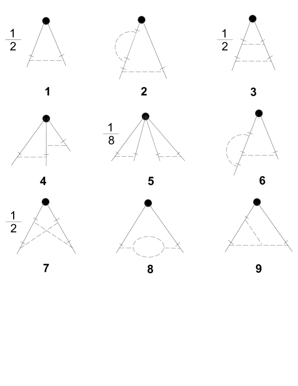
FIG. 1.: Diagrams of the function $\Gamma$ from (42) in the one-loop and two-loop approximations.

REFERENCES

- [1] A. S. Monin and A. M. Yaglom, Statistical Fluid Mechanics, Vol.2 (MIT Press, Cambridge, MA, 1975).
- [2] U. Frisch, Turbulence: The Legacy of A. N. Kolmogorov (Cambridge University Press, Cambridge, 1995).
- [3] K.R. Sreenivasan and R.A. Antonia, Annu. Rev. Fluid. Mech. 29 (1997) 435.
- [4] Z. Warhaft, Ann. Rev. Fluid Mech. 32, 203 (2000).
- [5] R.A. Antonia, E. Hopfinger, Y. Gagne, and F. Anselmet, Phys. Rev. A 30, 2704 (1984).
- [6] F. Moisy, H. Willaime, J.S. Andersen, and P. Tabeling, Phys. Rev. Lett. 86, 4827 (2001).
- [7] R.H. Kraichnan, Phys. Fluids 11, 945 (1968).
- [8] R.H. Kraichnan, Phys. Rev. Lett. 72, 1016 (1994).
- [9] K. Gawȩdzki and A. Kupiainen, Phys. Rev. Lett. 75, 3834 (1995); D. Bernard, K. Gawȩdzki, and A. Kupiainen, Phys. Rev. E 54, 2564 (1996).
- [10] M. Chertkov, G. Falkovich, I. Kolokolov, and V. Lebedev, Phys. Rev. E 52, 4924 (1995); M. Chertkov and G. Falkovich, Phys. Rev. Lett. 76, 2706 (1996).
- [11] A. Pumir, Europhys. Lett. 34, 25 (1996); 37, 529 (1997); Phys. Rev. E 57, 2914 (1998).
- [12] B.I. Shraiman and E.D. Siggia, Phys. Rev. Lett. 77, 2463 (1996); A. Pumir, B.I. Shraiman, and E.D. Siggia, Phys. Rev. E 55, R1263 (1997).
- [13] L.Ts. Adzhemyan, N.V. Antonov, and A.N. Vasil’ev, Phys. Rev. E 58, 1823 (1998); Theor. Math. Phys. 120, 1074 (1999).
- [14] G. Falkovich, K. Gawȩdzki, and M. Vergassola, Rev. Mod. Phys. 73, 913 (2001).
- [15] J. Zinn-Justin, Quantum Field Theory and Critical Phenomena (Clarendon, Oxford, 1989).
- [16] A.N. Vasil’ev, The Field Theoretic Renormalization Group in Critical Behavior Theory and Stochastic Dynamics (St Petersburg Institute of Nuclear Physics, St Petersburg, 1998) [in Russian; English translation: Chapman & Hall/CRC, Boca Raton, 2004].
- [17] L.Ts. Adzhemyan and N.V. Antonov, Phys. Rev. E 58, 7381 (1998); N.V. Antonov and J. Honkonen, E 63, 036302 (2001).
- [18] L.Ts. Adzhemyan, N.V. Antonov, V.A. Barinov, Yu.S. Kabrits, and A.N. Vasil’ev, Phys. Rev. E 63, 025303(R) (2001); E 64, 019901(E) (2001).
- [19] L.Ts. Adzhemyan, N.V. Antonov, V.A. Barinov, Yu.S. Kabrits, and A.N. Vasil’ev, Phys. Rev. E 64: 056306 (2001).
- [20] M. Vergassola, Phys. Rev. E 53, R3021 (1996); I. Rogachevskii and N. Kleeorin, Phys. Rev. E 56, 417 (1997).
- [21] A. Lanotte and A. Mazzino, Phys. Rev. E 60, R3483 (1999); I. Arad, L. Biferale, and I. Procaccia, Phys. Rev. E 61, 2654 (2000).
- [22] N.V. Antonov, A. Lanotte, and A. Mazzino, Phys. Rev. E 61, 6586 (2000); N.V. Antonov, J. Honkonen, A. Mazzino, P. Muratore-Ginanneschi, Phys. Rev. E 62, R5891 (2000); L.Ts. Adzhemyan, N.V. Antonov, A. Mazzino, P. Muratore-Ginanneschi, and A.V. Runov, Europhys. Lett. 55, 801 (2001).
- [23] L.Ts. Adzhemyan, N.V. Antonov, M. Hnatich, and S.V. Novikov, ibid., E 63, 016309 (2000); M. Hnatich, M. Jurčišin, A. Mazzino, and S. Šprinc, Acta Physica Slovaca 52, 559 (2002).
- [24] L.Ts. Adzhemyan and A.V. Runov, Vestnik SPbU, Ser. Phys. Chem., issue 1 (No 4), 85 (2001); L.Ts. Adzhemyan, N.V. Antonov, and A.V. Runov, Phys. Rev. E 64, 046310 (2001).
- [25] K.J. Wiese, J. Stat. Phys. 101, 843 (2000).
- [26] D. Bernard, K. Gawȩdzki, and A. Kupiainen, J. Stat. Phys. 90, 519 (1998).
- [27] A. Celani and M. Vergassola, Phys. Rev. Lett. 86, 424 (2001).
- [28] I. Arad, L. Biferale, A. Celani, I. Procaccia, and M. Vergassola, Phys. Rev. Lett. 87, 164502 (2001).
- [29] N.V. Antonov, Phys. Rev. E 60, 6691 (1999).
- [30] L.Ts. Adzhemyan, N.V. Antonov, and J. Honkonen, Phys. Rev. E 66, 036313 (2002).
- [31] N.V. Antonov, Physica D 144, 370 (2000).
- [32] N.V. Antonov, M. Hnatich, J. Honkonen, and M. Jurčišin, Phys. Rev. E 68, 046306 (2003).
- [33] M. Holzer and E.D. Siggia, Phys. Fluids 6, 1820 (1994).
- [34] B.I. Shraiman and E.D. Siggia, C.R. Acad. Sci., Ser. IIa: Sci. Terre Planets 321, 279 (1995).
- [35] M. Chertkov, G. Falkovich, and V. Lebedev, Phys. Rev. Lett. 76, 3707 (1996).
- [36] G. Eyink, Phys. Rev. E 54, 1497 (1996).
- [37] M. Avellaneda and A. Majda, Commun. Math. Phys. 131, 381 (1990); 146, 139 (1992); Q. Zhang and J. Glimm, ibid. 146, 217 (1992).
- [38] A. Majda, J. Stat. Phys. 73, 515 (1993); D. Horntrop and A. Majda, J. Math. Sci. Univ. Tokyo 1, 23 (1994).
- [39] K. H. Andersen and P. Muratore Ginanneschi, Phys. Rev. E 60: 6663 (1999).
- [40] A. Fannjiang, Physica D 136, 145 (2000); Erratum: 157, 166 (2001).
- [41] M. Chaves, K. Gawȩdzki, P. Horvai, A. Kupiainen, and M. Vergassola, J. Stat. Phys. 113, 643 (2003).
- [42] U. Frisch, A. Mazzino, and M. Vergassola, Phys. Rev. Lett. 80, 5532 (1998); U. Frisch, A. Mazzino, A. Noullez, and M. Vergassola, Phys. Fluids 11, 2178 (1999); A. Mazzino and P. Muratore-Ginanneschi, Phys. Rev. E 63, 015302(R) (2001).
- [43] L.Ts. Adzhemyan, N.V. Antonov and A.N. Vasil’ev, Zh. Éksp. Teor. Fiz. 95, 1272 (1989) [Engl. transl. Sov. Phys. JETP 68, 733 (1989)].
- [44] L.Ts. Adzhemyan, N.V. Antonov, and A.N. Vasil’ev, Usp. Fiz. Nauk, 166, 1257 (1996) [Phys. Usp. 39, 1193 (1996)].
- [45] L.Ts. Adzhemyan, N.V. Antonov, and A.N. Vasiliev, The Field Theoretic Renormalization Group in Fully Developed Turbulence (Gordon & Breach, London, 1999).
- [46] L.Ts. Adzhemyan, N.V. Antonov, M.V. Kompaniets, A. N. Vasil’ev, Int. J. Mod. Phys. B17, 2137 (2003).
- [47] D. Forster, D.R. Nelson, and M.J. Stephen, Phys. Rev. Lett. 36, 867 (1976); Phys. Rev. A 16, 732 (1977).
- [48] C. De Dominicis and P.C. Martin, Phys. Rev. A 19, 419 (1979); Progr. Theor. Phys. Suppl. No 64, 108 (1978).
- [49] P.L. Sulem, J.D. Fournier, and U. Frisch, Lecture Notes in Physics, 104, 321 (1979); J.D. Fournier and U. Frisch, Phys. Rev. A 19, 1000 (1983).
- [50] L.Ts. Adzhemyan, A.N. Vasil’ev, and Yu.M. Pis’mak, Theor. Math. Phys. 57, 1131 (1983).
- [51] L. Biferale, A.S. Lanotte, and F. Toschi, Phys. Rev. Lett. 92, 094503 (2004); L. Biferale, M. Cencini, A.S. Lanotte, M. Sbragaglia, and F. Toschi, New J. Phys. 6, 37 (2004).
- [52] A. Sain, Manu, and R. Pandit, Phys. Rev. Lett. 81, 4377 (1998).
- [53] P.C. Martin, E.D. Siggia, and H.A. Rose, Phys. Rev. A8, 423 (1973); H.K. Janssen, Z. Phys. B 23, 377 (1976); R. Bausch, H.K. Janssen, and H. Wagner, Z. Phys. B 24, 113 (1976); C. De Dominicis, Journ. de Phys. 37, Suppl.C1, 247 (1976).
- [54] D. Ronis, Phys. Rev. A 36, 3322 (1987); J. Honkonen and M.Yu. Nalimov, Z. Phys. B 99, (1996); M. Hnatich, J. Honkonen, D. Horvath, and R. Semancik, Phys. Rev. E 59, 4112 (1999); L.Ts. Adzhemyan, J. Honkonen, M.V. Kompaniets, and A.N. Vasil’ev, Phys. Rev. E 68, 055302(R) (2003); E-print LANL nlin.CD/0407067 (Submitted to Phys. Rev. E).
- [55] L.Ts. Adzhemyan, Yu.S. Kabrits, M.V. Kompaniets, and A.N. Vasil’ev, Vestnik SPbU, Ser. 4, issue 1 (No 4), 3 (2000) [in Russian]; L.Ts. Adzhemyan, N.V. Antonov, M.V. Kompaniets, and A.N. Vasil’ev, Acta Physica Slovaca, 52, 565 (2002).
- [56] L.Ts. Adzhemyan, A.N. Vasil’ev, and M. Hnatich, Theor. Math. Phys. 58, 47 (1984).
- [57] V. Yakhot, S.A. Orszag, Phys. Rev. Lett. 57, 1722 (1986); Journ. Sci. Comp. 1, 3 (1986); W.P. Dannevik, V. Yakhot, S.A. Orszag, Phys. Fluids 30, 2021 (1987); É.V. Teodorovich, Prikladnaja Matematika i Mehanika 52, 218 (1988) [in Russian].
- [58] J.D. Fournier, P.L. Sulem, and A. Pouquet, J. Phys. A 15, 1393 (1982); L.Ts. Adzhemyan, A.N. Vasil’ev, and M. Hnatich, Theor. Math. Phys. 64, 777 (1985).
- [59] A. N. Vasiliev, Functional Methods in Quantum Field Theory and Statistics (Leningrad University Press, Leningrad, 1976) [In Russian; English translation: Gordon & Breach, London, 1998].
- [60] I. Arad, B. Dhruva, S. Kurien, V.S. L’vov, I. Procaccia, and K.R. Sreenivasan, Phys. Rev. Lett. 81, 5330 (1998); I. Arad, L. Biferale, I. Mazzitelli, and I. Procaccia, ibid., 82, 5040 (1999); S. Kurien, V.S. L’vov, I. Procaccia and K.R. Sreenivasan, ibid., E 61, 407 (2000); L. Biferale, I. Daumont, A. Lanotte, and T. Toschi, ibid., E 66, 056306 (2002); L. Biferale, E. Calzavarini, T. Toschi, and R. Tripiccione, Europhys. Lett. 64, 461 (2003)
- [61] G.L. Eyink, Phys. Lett. A 172, 355 (1993).
- [62] B. Duplantier and A. Ludwig, Phys. Rev. Lett. 66, 247 (1991).
- [63] M. Lässig, Phys. Rev. Lett. 84, 2618 (2000).
- [64] R.H. Kraichnan, Phys. Fluids A30, 2400 (1987); S. Chen and R.H. Kraichnan, ibid., A1, 2019 (1989).
- [65] L.Ts. Adzhemyan, A.N. Vasil’ev, and M. Hnatich, Theor. Math. Phys. 74, 115 (1988); L.Ts. Adzhemyan, N.V. Antonov, and T. L. Kim, ibid., 100, 1086 (1994); L.Ts. Adzhemyan, S.V. Borisenok, and V.I. Girina, ibid., 105, 1556 (1995); N.V. Antonov, S.V. Borisenok, and V.I. Girina, ibid., 106, 75 (1996); N.V. Antonov and A.N. Vasil’ev, ibid., 110, 97 (1997).
- [66] G. Falkovich, I. Kolokolov, V. Lebedev, and A. Migdal, Phys. Rev. E 54, 4896 (1996).
- [67] M. Chertkov, Phys. Rev. E 55, 2722 (1997); E. Balkovsky and V. Lebedev, ibid., E 58, 5776 (1998).
- [68] J. Honkonen, M.V. Komarova, and M.Yu. Nalimov, E-print LANL nlin.CD/0406168 (Submitted to Nucl. Phys. B).