Multifractal nature of plume structure in high Rayleigh number convection

Abstract

The geometrically different plan forms of near wall plume structure in turbulent natural convection, visualised by driving the convection using concentration differences across a membrane, are shown to have a common multifractal spectrum of singularities for Rayleigh numbers in the range $10^{10}-10^{11}$ at Schmidt number of 602. The scaling is seen for a length scale range of $2^{5}$ and is independent of the Rayleigh number, the flux, the strength and nature of the large scale flow, and the aspect ratio. Similar scaling is observed for the plume structures obtained in the presence of a weak flow across the membrane. This common non trivial spatial scaling is proposed to be due to the same underlying generating process of the near wall plume structures.

1 Introduction

Turbulent Rayleigh - Bénard convection and other related natural convection flows at high Rayleigh numbers have many unresolved issues; these are extensively discussed in the review of Siggia (1994). As most high $Ra$ studies are conducted in cryogenic conditions Niemela, Skrbek, Sreenivasan & Donelly (2000), which prevent visualisation of the near wall structures, little is known about the nature of near wall coherent structures in high Rayleigh number turbulent free convection. The non-dimensional parameters that characterise natural convection flows are the Rayleigh number ($Ra=g\frac{\Delta\rho}{\rho}H^{3}/\nu\kappa$, the ratio of buoyancy effects to dissipative effects); Prandtl number ($Pr=\nu/\kappa$ , a fluid property); Nusselt number ( $Nu=\frac{Q}{\kappa\Delta T/H}$, a non-dimensional flux) and aspect ratio (AR = $L/H$ , a geometric parameter of the fluid layer) where, $g$ = the acceleration due to gravity, $\frac{\Delta\rho}{\rho}$ = nondimensional density difference, $Q$ = the kinematic heat flux, $\Delta T$ = the temperature difference between the walls, $H$ = fluid layer height, $L$ = fluid layer width, $\nu$= kinematic viscosity and $\kappa$ = thermal diffusivity.

Most of the previous studies on near wall coherent structures give only a qualitative picture of closed polygonal forms of line plumes at $Ra\sim 10^{6}$, that change to randomly moving and merging line plume patterns at higher $Ra$ of $10^{7}-10^{8}$ Spangenberg & Rowland (1961); Tamai & Asaeda (1984); Theerthan & Arakeri (2000); Kerr & Herring (2000). Line plumes are buoyant fluid rising in the form of sheets from lines on the horizontal heated surface. Visualisations at the highest $Ra$ so far ($\sim 10^{9}$) by Zocchi, Moses & Libchaber (1990) show line plumes being swept along the direction of shear caused by the large scale flow. Theerthan & Arakeri (1998) showed that the randomly spaced and oriented plumes near the wall can be modeled as a regular array of laminar line plumes, each plume fed by laminar natural convection boundary layers on either side. Puthenveettil (2004) extended the analysis to high $Ra$- high $Pr$ case, and found that the probability distribution of plume spacings have a common log-normal form, independent of the parameter values. None of these studies address the spatial scaling of the plume structure pattern.

In this paper, we report the spatial scaling of the near wall plan-form plume structures in high Rayleigh number turbulent free-convection, using multifractal formalism. Briefly, multifractal formalism describes the statistical properties of singular measures in terms of the singularity spectrum $f(\alpha)$, corresponding to the singularity strength $\alpha$. $f(\alpha)$ can be regarded as the fractal dimensions of subsets with corresponding singularity strength $\alpha$. The details of multifractal formalism can be seen in  Mandelbrot (1989); Meneveau & Sreenivasan (1991); Halsey, Jensen, Kadanoff, Procaccia & Shraiman (1986), and the references cited therein. Even though studies abound on applying this formalism for characterising spatial structures in various fields, we are not aware of such an analysis of near wall coherent structures of turbulent convection.

2 Experimental setup and image preprocessing

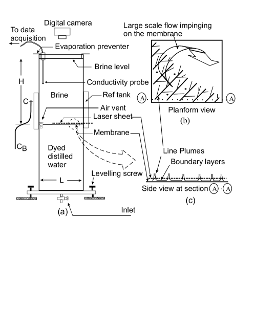
Figure 1: (a) The experimental set up (b) The plan form view of the near wall plume structure as seen at the intersection of a horizontal laser sheet. (c) The side view in a vertical plane showing rising line plumes. Planform in (b) is for the TF-type convection showing a plume free area where the large scale flow impinges on the membrane.

We visualise the near wall plume structure at high $Ra$ by driving the convection using concentration differences of NaCl across a membrane. Concentration in the present experiments is equivalent to temperature in Rayleigh - Bénard convection. High $Ra$ ($10^{10}-10^{11}$) are achieved at Schmidt number ($Sc$ $\sim\nu/D$, equivalent to $Pr$) of 602 due to the low molecular diffusivity of NaCl. The set-up consists of two glass compartments of square cross section, arranged one on top of the other with a fine membrane fixed horizontally in between them; the schematic is shown in Figure 1. The membranes used are Pall Gelmann™NX29325 membrane disc filters (PG henceforth) with a random pore structure having a mean pore size of $0.45\mu$ and Swedish Nylobolt 140S screen printing membrane (140s henceforth) with a regular square pore of size $35\mu\times 35\mu$.

The bottom tank is filled with distilled water tagged with a small amount of Sodium Fluoresceine (absorption spectra peak at 488nm and emission spectra peak at 518nm) and then the top tank filled with brine to initiate the experiment. The convection is unsteady, but quasi-steady approximation can be used as the time scale of change of the density difference $(\frac{\Delta\rho}{\rho}/\frac{d\frac{\Delta\rho}{\rho}}{dt})$ is 10 times the time scale of one large scale circulation $(H/W_{*})$, where $W_{*}\sim\left(g\beta QH\right)^{1/3}$Deardorff (1970) is an estimate of the large scale flow strength, H is the top tank fluid layer height, $Q$ denotes the flux of NaCl and $\beta$ is the coefficient of salinity. A horizontal laser sheet, expanded and collimated from a 5W Spectra Physics Stabilite™2017 Ar- Ion laser at 488nm is passed just above ($<$1 mm) the membrane. The dye in the bottom solution while convecting upward fluoresces on incidence of the laser beam to make the plume structure visible. A schematic of the visualisation of the near wall phenomena is shown in Figure 1(b) and (c). A visible long pass filter glass, Coherent optics OG-515, is used to block any scattered laser light and allow the emitted fluorescence to pass through. The images are captured on a digital handycam Sony DCR PC9E. Experiments are conducted in 23 cm high tanks, with one tank having 15 cm$\times$15 cm (AR = 0.65) cross section and another with 10 cm$\times$10 cm (AR = 0.435) cross section. Starting top tank NaCl concentrations of 10g/l, 7g/l and 3g/l are used to study the plume structure under different $Ra$.

The Laser Induced Fluorescence (LIF) images are RGB 24bit color with 640 $\times$ 480 pixels resolution. The multifractal analysis is conducted on binary images obtained from these RGB images. In using binary images, we are neglecting the intensity variation of the fluorescence (proportional to the concentration of the dye) within the plume line thickness. The analysis is hence valid only for the geometrical aspects of the planform. A similar telegraph approximation of the temperature time trace measured at the middle of the fluid layer has been studied by Bershadskii, Niemela, Praskovsky & Sreenivasan (2004) to show the clusterisation of plumes. The RGB image is cropped to remove the tank walls, converted to gray scale, Radon transformed to remove the lines (formed due to imperfections in the optics and the test section surface) and then re-sampled to increase the resolution. The non-uniform background illumination due to the attenuation of the laser sheet is subtracted to obtain the plume lines over a uniform dark background. Contrast and intensity are enhanced to make the plume lines clearer before converting to a black and white binary image using a threshold. The effect of thresholding on the multifractal exponents is considered in Appendix A. The binary image retains almost all the features of the raw image.

3 The plume structure planforms

(a) PG membrane in 15 cm$\times$15 cm tank, $Ra$ = 2.04$\times 10^{11}$, $\Delta C$ = 3.2 g/l, $Q$ = 0.1 mg/cm²/min, $W_{*}$ = 0.31 cm/s, $Re$=797, Image area = 14.65cm square, 714²pix

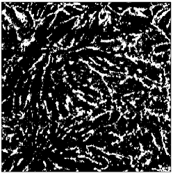
(b) Structure after 30seconds from (a) $Ra$ = 2.03$\times 10^{11}$, $\Delta C$ = 3.19 g/l, $Q$ = 0.1 mg/cm²/min, $W_{*}$ = 0.31 cm/s, $Re$ = 797, Image area = 13.74 cm square, 728² pix

(c) PG membrane in 10 cm$\times$10 cm tank, $Ra$ = 2.03$\times 10^{11}$, $\Delta C$ = 3.198 g/l, $Q$ = 0.11 mg/cm²/min, $W_{*}$ = 0.31cm/s, $Re$ = 797, Image area = 9.157 cm square, 728² pix

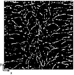
(d) PG membrane in 15 cm$\times$15 cm tank, $Ra$ = 5.56$\times 10^{10}$, $\Delta C$ = 0.875 g/l, $Q$ = 0.02 mg/cm²/min, $W_{*}$ = 0.18cm/s, $Re$ = 463.6, Image area = 12.83cm square, 728² pix

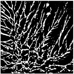
(e) 140s membrane in 15 cm$\times$15 cm tank, $Ra$ = 5$\times 10^{11}$, $\Delta C$ = 7.87 g/l, $Q$ = 0.39 mg/cm²/min, $W_{*}$ = 0.47 cm/s, $Re$ = 1210.5, $V_{I}$ = 0.002 cm/s, Image area = 8.61 cm square, 528²pix

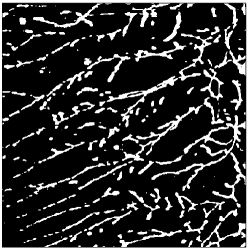
(f) 140s membrane in 15 cm$\times$15 cm tank, $Ra$ = 4.49$\times 10^{11}$, $\Delta C$ = 7.06 g/l, $Q$ = 0.41 mg/cm²/min, $W_{*}$ = 0.48 cm/s, $Re$ = 1236.3, $V_{I}$ = 0.0023 cm/s, Image area = 8.32 cm square, 520² pix

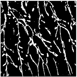
(g) 140s membrane in 15 cm $\times$15 cm tank, $Ra$ = 5.36$\times 10^{11}$, $\Delta C$ = 8.42g/l, $Q$ = 0.41 mg/cm²/min, $W_{*}$ = 0.48 cm/s, $Re$ = 1236.3, $V_{I}$ = 0.0016 cm/s, Image area = 7.58 cm square, 616² pix

(h) 140s membrane in 15 cm$\times$15 cm tank, $Ra$ = 1.65$\times 10^{11}$, $\Delta C$ = 2.6 g/l, $Q$ = 0.07 mg/cm²/min, $W_{*}$ = 0.27cm/s, $Re$ = 695.4, Image area= 14.69 cm square, 714² pix

Figure 2: The plan forms of near wall plume structures obtained under different conditions. (a)to (d) are for the D-Type showing full tank cross section. (e) to (g) show the planforms of the plume occupied region in the TF-type convection. (e) shows the corner area with the walls only on the left and the bottom of the image. (f) shows the corner portion with the walls on the top and the right. (g) shows a zoomed view of the central shear dominant portion. (h) shows the structure when the D-type occurs in the coarser membrane at lower driving potentials

Figure 2 shows the binary images of the various planform plume structures obtained in the experiments. The parameter values are shown below each image. $\Delta C$(g/l) is the effective driving concentration difference on the side of the membrane where the structure is visualised; $Ra$ is based on this $\Delta C$. The white lines in the figures, of thickness $\sim 1$mm, are the bases of the sheet plumes originating from the membrane surface. Two types of convection are observed depending on the pore size of the membrane. In one case, the transport of salt through the membrane is by diffusion (D-type henceforth). In the second case, the transport is due to a flow, albeit weak, across the membrane (TF type henceforth). In both cases, the line plumes emanate from the thin unstable boundary layers above the membrane. As the focus of this paper is on the spatial scaling of these structures, we give only a brief description of the phenomena in each image of Figure 2; the details are discussed in Puthenveettil (2004).

3.1 Planforms in D-Type convection

For the lower pore sized (PG $0.45\mu$) membrane, the transport across the partition is diffusion dominated, while the transport above and below the membrane is similar to Rayleigh - Bénard convection at high $Ra$. Figures 2(a) to 2(d) show the structures obtained in the D-type convection. Similar plumes cover the cross section on the lower side of the membrane. The first two images are from the larger AR =0.65 which had multiple large scale flow cells, the signatures of which are seen as circular patches with aligned line plumes oriented radially around the patches, the plume free circular patch being the area where the large scale circulation impinges on the membrane. The diffusion layer thickness $\delta=D\Delta C/Q$ is about 0.26 mm for the image of Figure 4(a). The large scale flow cells shift their position at a larger time scale ($\sim$ 20 min) than one large scale circulation time ($\sim$ 1 min), which is greater than the time scale of few seconds for the merging of plumes. Figure 2(c) shows the planform of plume structure under the same conditions as in Figures  2(a) and 2(b), but in the smaller (10 cm $\times$ 10 cm, AR=0.435) cross sectional area tank. In this case, there was only a single large scale circulation which was rotating clockwise in the $x-z$ plane and aligning the near wall plumes in the $x$-direction (See Figure 2(d) for the co-ordinate directions, $z$ is normal to the membrane). The plume structure at lower $Ra$ in the larger AR =0.65 tank, shown in Figure  2(d), had two counter rotating circulation cells ( anticlockwise on the left and clockwise on the right) rotating in the $x-z$ plane which created a near wall mean shear directed toward the center along the $x$ direction. In all these images, the flux scaled approximately as $\Delta C^{4/3}$, equivalent to $Nu\sim Ra^{1/3}$ in turbulent Rayleigh - Bénard convection.

3.2 Planforms in TF-Type convection

Experiments with the coarser ($140s,\,35\mu$) membrane showed that only half the area above the membrane was covered by plumes, with the other half having plumes below the membrane. This structure is due to a weak through flow across the membrane. The lower fluid dynamic resistance of the coarser membrane allows this through flow. The region having plumes on top of the membrane corresponds to upward through flow and vice versa ( Figure 1(b)). The through flow velocities $V_{I}$ are about 10 times smaller than the near wall velocity scales in turbulent free convection given by $W_{o}\sim\left(g\beta QD\right)^{1/4}$Townsend (1959). Figure 2(e) to 2(g) show the plan form view of the plume occupied region in the TF type convection at AR =0.65. Figure 2(e) shows the corner region of this structure when there was a near wall mean shear toward the bottom left corner due to a diagonally oriented large scale circulation rotating in the clockwise direction. Figure 2(f) shows a similar corner view of the structure when there is a near wall mean shear along the diagonal toward the top right corner, created by an anticlockwise circulation. The central zoomed view, where the mean shear effects are predominant, in a structure similar to that in Figures 2(e) and 2(f), is shown in Figure 2(g). In all these cases, the flux scaled as $\Delta C^{3}$ due to the presence of a flow across the membrane. The phenomenology behind this flux scaling is described in Puthenveettil (2004). At lower driving potentials, the TF-type convection in the 140s membrane experiments was seen to change to the D-type with $Q\sim\Delta C^{4/3}$ scaling. Figure 2(h) shows one such type of plume structure.

In both the types of convection, the plume structures are continuously evolving spatio-temporal patterns. But, as the time scale of the merging of plumes is much smaller than the time scale of change of Rayleigh number, the planforms could be expected to exhibit statistically stationary characteristics for a given set of parameters. In addition, the scale free, non uniform and dendritic appearance, along with the the common probability distribution of the spacings, motivated us to analyse the structures using multifractal analysis.

4 Multifractal analysis

4.1 Methodology and Scaling range

We use the standard box counting methodology to estimate the multifractal exponents. The analysis is done on square binary images (L² pixels). The measure $P_{i,j}$ where, $i,j$ are the box indices, is the probability of occurrence of the plume in a box, calculated as the ratio of white pixels in each box to the total number of white pixels in the image. For each moment $q$, the partition function $Z_{q}=\sum_{i,j}P_{i,j}^{q}$ is calculated for various box sizes ($l_{b}$ in pixels). The slope of $\ln Z_{q}$ Vs $\ln\left(\frac{l_{b}}{L}\right)$ gives the Cumulant generating function $\tau(q)$ defined through $\sum_{i,j}P_{i,j}^{q}\sim\left(\frac{l_{b}}{L}\right)^{\tau(q)}$ where, $\tau(q)=(q-1)D_{q}$ with $D_{q}$ referring to $q^{th}$ order Renyi dimension. The number of boxes where $P_{i,j}\sim\left(\frac{l_{b}}{L}\right)^{\alpha}$ has a singularity strength between $\alpha$ and $\alpha+d\alpha$ is given by $N(\alpha)\sim\left(\frac{l_{b}}{L}\right)^{-f(\alpha)}$. $f(\alpha)$ is the fractal dimension of the subset - picked out by each value of the moment $q$ - with singularity strength $\alpha$. We calculate the Hölder exponent $\alpha$ and $f(\alpha)$ using the direct method due to  Chabra & Jensen (1989). The expressions for $f(\alpha)$ and $\alpha$ are $f(q)\,=\,\lim_{l_{b}\rightarrow 0}\frac{\sum_{i,j}\mu_{i,j}\,\ln\,\mu_{i,j}}{\ln(l_{b}/L)},\qquad\alpha(q)\,=\,\lim_{l_{b}\rightarrow 0}\frac{\sum_{i,j}\mu_{i,j}\,\ln\,P_{i,j}}{\ln(l_{b}/L)},$where $\mu_{i,j}\,=\,\frac{P_{i,j}^{q}}{\sum_{i,j}P_{i,j}^{q}}$ are the normalized measures. For each value of the moment $q$, the slope of the of the plots of the numerator vs the denominator in the expressions for $f(q)$ and $\alpha(q)$, in the range of values where the plots are linear, give $f(q)$ and $\,\alpha(q)$. In our work, the range of $q$ values is limited to $-2\leq q\leq 5$ in order to have a reasonable range of scaling regime.

The estimation of $f(\alpha)$ and $\alpha$ for the image in Figure 2(e) is shown in Figure 3. The image size is 8.61 cm square sampled at 528² pixels (L= 528). The calculation is done for box sizes $l_{b}$ = 528, 264, 176, 132, 88, 66, 48, 44, 33, 24 and 22 pixels. Figure 3(a) shows the plots of $\sum_{i,j}\mu_{i,j}\,\ln\,\mu_{i,j}$ versus $\ln(l_{b}/L)$ for a few typical values of $q=-2,0.5$ and 5. The slope of the linear fit in the range 66 pix $\leq l_{b}\leq$ 528 pix, (i.e., from 1.076 to 8.61 cm) is used to estimate $f(\alpha(q))$ for all q. This slope is valid for a larger length scale range of 22 pix $\leq l_{b}\leq$ 528 pix, (i.e. from 0.359 to 8.61 cm ) for $q$ =-0.5 and 5.0, while for $q$ = -2, the linearity holds only in the fit range. The same linearity ranges for various $q$ values are used for estimating $\alpha(q)$ from the plot of $\sum_{i,j}\mu_{i,j}\,\ln\,P_{i,j}$ vs $\ln(l_{b}/L)$ (Figure 3(b)) and $\tau(q)$ from the plots of $\ln\sum_{i,j}P_{i,j}^{q}$ vs $\ln(l_{b}/L)$ (Figure 3(c)). Figure 3(a) to 3(c) show that the deviation from the linearity is pronounced for $q=-2$ below a specific box size of around 1cm ($\ln(l_{b}/L)=-2$), while it is almost negligible for positive moments. This behavior is also seen in other studies like Chabra, Meneveau, Jensen & Sreenivasan (1989) and Meneveau & Sreenivasan (1991). As negative moments amplify low measures, and the effect of noise in the low measure regions at smaller box sizes is substantial, we expect this deviation to be due to the amplification of the errors. For the same reason, the negative moment slopes were also the most affected when the binary image threshold was changed (See inset of Figure 7).

The analysis is carried out for all the images in Figure 2. The major common observations from the plots of $\sum_{i,j}\mu_{i,j}\ln\mu_{i,j}$ and $\sum_{i,j}\mu_{i,j}\ln P_{i,j}$ vs $\ln(l_{b}/L)$ for these images are as follows. (a) For moments $q\geq-1$, the linearity of the above quantities is seen to hold till about 0.5 cm. As positive moments pick out areas of higher measure, these moments represent the main plume structure. Thus, the main plume structure shows a multifractal scaling in the range of tank cross section to 0.5 cm i.e., a range of $2^{5}$. (b) When negative moments are less than -1, the plots of these quantities show a deviation from linearity at about 1 cm in all the images. Hence, for $q<-1$, the multifractal scaling is valid for a shorter length scale range of tank cross section to 1 cm, i.e. $\sim 2^{4}$. (c) There seems to be a further lower cut off of approximately 5 mm, below which the slope of $\sum_{i,j}\mu_{i,j}\ln P_{i,j}$ Vs $l_{b}/L$ for $q\leq 1$ goes to zero (See Figure 3(b) at $\ln(l_{b}/L)\sim-2.75$). This is expected to be because the box sizes have reached the same order as the plume spacings. The geometric structure of the planform does not exist below this length scale.

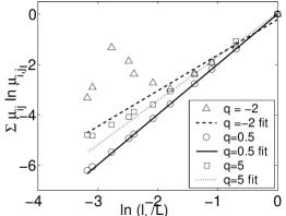
(a) Range for $f(\alpha)$

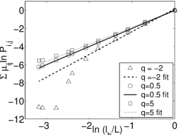
(b) Range for $\alpha$

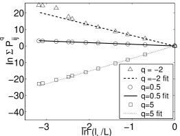
(c) Range for $\tau(q)$

Figure 3: The range of multifractal scaling for moments q = -2, 0.5 and 5. The lines show the linear fit used for calculating the slopes.

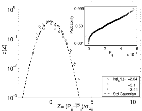
Figure 4: The probability distribution function of the measure $P_{i,j}$ in the standardised form at three box sizes. The inset shows the normal probability plot of the measure at the intermediate box size.

To understand the above behaviour, we studied the probability distribution function of the measures at various box sizes. The distribution function of the measures is described by its moments $Z_{q}$, and hence is related to $\tau(q)$ through $Z_{q}\sim\left(l_{b}/L\right)^{\tau(q)}$. The distributions of $P_{ij}$ in the standardised form $Z=\left(P_{ij}-\overline{P_{ij}}\right)/\sigma_{P_{ij}}$ for Figure 2(h), where $\overline{P_{ij}}$ indicates the mean and $\sigma_{P_{ij}}$ the standard deviation, for three box sizes are shown in Figure 4. The measure is distributed normally for the larger box sizes. With decreasing box sizes, the low measure and the high measure tails of the distribution deviates from the Gaussian. This is clear from the inset in Figure 4, which shows the normal probability plot of $P_{ij}$ for the intermediate box size; the deviation from linearity shows the difference from the Gaussian. All the images in Figure 2 showed similar form and behaviour of the probability distribution of the measures. The deviation from linearity for negative moments in Figure 3 at smaller box sizes seems to be consistent with the deviation of the low measure tails of the distribution function in Figure 4.

4.2 The multifractal spectrum

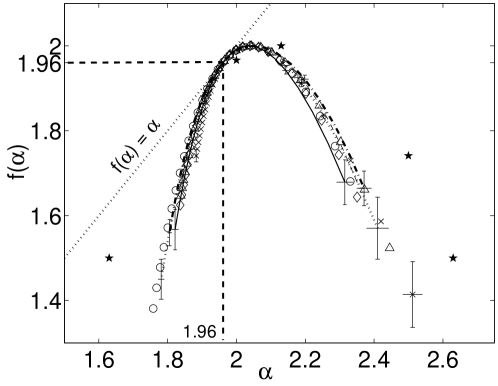
Figure 5: The $f-\alpha$ spectrum for all the images. …. Figure 2(a), -.-.- Figure 2(b), $\circ$ Figure 2(c), — Figure 2(d), $\times$ Figure 2(e), $\lozenge$ Figure 2(f), $\bigtriangleup$ Figure 2(g), - - - Figure 2(h), $\star$ Meneveau & Sreenivasan (1991).

$q$	-2.0	-1.5	-1.0	-0.5	0	0.5	1.0	1.5	2.0	2.5	3.0	3.5	4.0	4.5	5.0
$D_{q}$	2.13	2.09	2.05	2.02	2.0	1.98	1.96	1.95	1.93	1.92	1.91	1.897	1.886	1.875	1.86

Table 1: Variation of the Renyi dimension $D_{q}$ with the moment $q$ for Figure 2(a)

The $f-\alpha$ curves of all the images in Figure 2 are shown in Figure 5. The error bars in the figure are the errors in the slope of the linear curve fits. The value of $f$ at $q\,=\,0$ is the fractal dimension of the ‘support’ of the measure. As the underlying area over which the plumes are formed is a non-fractal surface, $f(\alpha(0))\,=\,2$. Figure 5 shows that this is satisfied, suggesting a good level of confidence in the calculation. We also note that the fractal dimension corresponding to the (information) entropy $S\,=\,\sum_{\beta=0}^{b-1}p_{\beta}\log_{b}p_{\beta},$ of the underlying process which generates these structures is 1.96. The corresponding values $D_{q}$ for Figure 2(a) are shown in Table 1.

The results of our analysis of the near wall plume structure in turbulent free-convection at high $Ra$ are strongly suggestive of its multifractal nature. The analysed images cover a wide range of conditions viz., $Ra$ range of about a decade, different test section cross sectional areas (10$\times$10 cm² and 15$\times$15 cm²), absence and presence of a flow through the membrane, different large scale flow strengths (about 2.5 times), a wide range of flux (over two decades) and show a wide variety of structures having single and multiple large scale flow cells with aligned and random structures. The plot of Figure  5 show that, within the errors encountered in the current analysis, all these images have the same multifractal scaling of the main plume structure for length scales greater than 0.5cm.

5 Discussion and Conclusions

We have shown that the plan forms of near wall plume structure in high $Ra$ turbulent free-convection under varying parameter values have the same multifractal spectrum of singularities. Even though the plan forms appear substantially different in their geometric form, they have the same non trivial spatial scaling. The probabilistic interpretation of multifractal formalism, as described by Mandelbrot (1989), shows that $f$ and $\alpha$ indirectly describe the underlying generating mechanism of these structures in terms of the multipliers $M$ for each stage of the process. These exponents are independent of the length scales and are unique functions of the multiplier distribution which decides how the measure is distributed at each stage. Figure 6 shows the probability distribution of the multipliers in the standardised form, $\chi=\left(M-\overline{M}\right)/\sigma_{M}$. The multiplier values are calculated as the ratio of the measures in each box to the measure in its parent box, when each box divides into four boxes. The calculations are done for a series of box sizes as shown in the legend of the Figure 6. The figure shows that the image has the same form of distribution function of multipliers at different length scales, which has an exponential tail of higher multipliers. Note that the length scale spans the entire range over which $f(\alpha)$ has been obtained. Similar results were obtained for all the images in Figure 2. In physical terms, this means that the present images have the same underlying generating mechanism. The common generating mechanism that can be identified here is that the thin boundary layers of lighter fluid above the membrane becomes unstable resulting in the generation of sheet plumes. Interaction of the neighboring plumes due to entrainment leads to their merger. New plumes are nucleated in the vacant space due to the merger. The whole process is also influenced by the external flow field created by the mean wind, whose effect is to align the plume lines in the direction of the mean shear.

An identical probability distribution of multipliers at different stages of the process would show that the multipliers at different stages are not correlated and the underlying process to be statistically self similar  Mandelbrot (1989); Chabra & Sreenivasan (1992); Frederiksen, Dahm & Dowling (1997). The inset in Figure 6 shows the probability distribution function of the multipliers, shown only at two box sizes for clarity. The distribution functions coincide at larger multiplier values for the whole multifractal range, but are different at low multiplier values. We expect this to be a due to the correlated nature of the ends of the structure (low multipliers), which move towards the main plume lines due to entrainment.

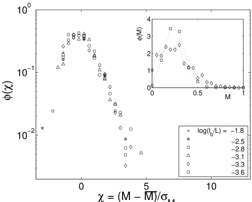
Figure 6: The probability distribution function of the standardised form of the multipliers at different box sizes. The inset shows the distribution function of multipliers at two box sizes.

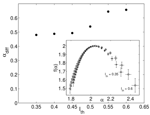
Figure 7: The variation of $\alpha_{diff}=\alpha_{max}-\alpha_{min}$ with the threshold $I_{th}$ for Figure 2(d). The inset shows the $f-\alpha$ curve for the two extreme thresholds

Recall that for multinomial processes, $f(\alpha)$ is calculated as the maximum from a range of values for any $\alpha$ for each moment $q$. Connecting this with the thermodynamic analogy noted in the literature Chabra et al. (1989), the common $f-\alpha$ curves might imply that the plume structure in turbulent convection is formed so as to maximize the entropy of the structure.

Earlier studies on the multifractal nature of energy dissipation field in turbulent flows by Meneveau & Sreenivasan (1991) have parallels with the current study. The energy dissipation is caused by the velocity gradients at the viscous scales. Plume edges represent the major gradients of velocities near the wall in convection. These also are the relevant viscous scales near the wall. Hence, it is possible that the near wall energy dissipation field follows the plume structure closely. The $f-\alpha$ curves obtained by Meneveau & Sreenivasan (1991) are shown in comparison with the present curves in Figure 5. The $f(\alpha)$ curves obtained in our case have a lower spread. Further work is needed to clarify the possible connection of these energy dissipation studies to the present analysis.

Appendix A Effect of thresholding

The robustness of the calculated multifractal exponents depends on how representative the binary image is of the RGB LIF image. Figure 7 shows the variation of $\alpha_{diff}=\alpha_{max}-\alpha_{min}$ with the threshold $(0\leq I_{th}\leq 1)$ for the image in Figure 2(d). The inset in Figure 7 shows the $f-\alpha$ curves at the two extreme thresholds. $I_{th}\geq 0.55$ produced binary images clearly missing in finer details, while $I_{th}\leq 0.45$ created images that were noisier, with larger plume thickness. Therefore, for this image, the threshold was chosen to be 0.45. The variation of $\alpha_{diff}$ for $0.45\geq I_{th}\leq 0.55$ is about 0.15, of the same order as the error in $\alpha$. Therefore, the change in the $\alpha$ due to the error from the optimum threshold is within the error involved in the calculation of $\alpha$. Further, the inset of Figure 7 shows that the threshold does not affect the form of the $f-\alpha$ curve. Hence in all the images, the threshold was chosen by visual judgment along with sensitivity analysis. The above analysis was for one of the low quality images; for better quality images as in Figure 2(f), there was negligible variation with threshold.

We thank G.Vishwanath and Joby Joseph for assistance related to image processing and K.R.Sreenivasan for his comments on the draft version.

References

- Bershadskii et al. (2004) Bershadskii, A., Niemela, J., Praskovsky, A. & Sreenivasan, K. 2004 “Clusterisation” and intermittency of temperature fluctuations in turbulent convection. Physical Review E 69, 056314.
- Chabra et al. (1989) Chabra, A., Meneveau, C., Jensen, R. & Sreenivasan, K. R. 1989 Direct determination of the ) singularity spectrum and it application to fully developed turbulence. Physical Review A 40 (9), 5284–5294.
- Chabra & Jensen (1989) Chabra, A. B. & Jensen, R. V. 1989 Direct determination of ) singularity spectrum. Physical Review Letters 62 (12), 1327–1330.
- Chabra & Sreenivasan (1992) Chabra, A. B. & Sreenivasan, K. R. 1992 Scale invariant multipliers in turbulence. Physical Review Letters 68 (18), 2762.
- Deardorff (1970) Deardorff, J. 1970 Convective velocity and temperature scales for the unstable planetary boundary layer and for Rayleigh convection. Journal of the Atmospheric Sciences 27, 1211–1213.
- Frederiksen et al. (1997) Frederiksen, R. D., Dahm, W. & Dowling, D. 1997 Experimental assessment of fractal scale similarity in turbulent flows. part 3. multifractal scaling. Jl. Fluid. Mech. 338, 127–155.
- Halsey et al. (1986) Halsey, T., Jensen, M., Kadanoff, L., Procaccia, I. & Shraiman, B. 1986 Fractal measures and their singularities:the characterisation of strange sets. Physical Review A 33 (2), 1141–1151.
- Kerr & Herring (2000) Kerr, R. M. & Herring, J. R. 2000 Prandtl number dependence of nusselt number in direct numerical simulations. Jl. Fluid. Mech. 419, 325–344.
- Mandelbrot (1989) Mandelbrot, B. B. 1989 Multifractal measures, especially for the geophysicist. Pure and applied geophysics 131 (1/2), 5–42.
- Meneveau & Sreenivasan (1991) Meneveau, C. & Sreenivasan, K. R. 1991 The multifractal nature of turbulent energy dissipation. Jl. Fluid. Mech. 224, 429–484.
- Niemela et al. (2000) Niemela, J., Skrbek, L., Sreenivasan, K. & Donelly, R. 2000 Turbulent convection at very high Rayleigh numbers. Nature 404, 837–840.
- Puthenveettil (2004) Puthenveettil, B. A. 2004 Investigations on high Rayleigh number turbulent free-convetion. PhD thesis, Indian Institute of Science, Bangalore, http://www.mecheng.iisc.ernet.in/~apbabu/resinfo.htm.
- Siggia (1994) Siggia, E. D. 1994 High Rayleigh number convection. In Ann Rev Fluid Mechanics, , vol. 26, pp. 137–168.
- Spangenberg & Rowland (1961) Spangenberg, W. G. & Rowland, W. G. 1961 Convective circulation in water induced by evaporative cooling. Phys. Fluids 4 (6), 743–750.
- Tamai & Asaeda (1984) Tamai, N. & Asaeda, T. 1984 Sheet like plumes near a heated bottom plate at large Rayleigh number. Jl. Geophys. Res. 89, 727–734.
- Theerthan & Arakeri (1998) Theerthan, S. A. & Arakeri, J. H. 1998 A model for near wall dynamics in turbulent Rayleigh - Bénard convection. Jl. Fluid. Mech. 373, 221 –254.
- Theerthan & Arakeri (2000) Theerthan, S. A. & Arakeri, J. H. 2000 Plan form structure and heat transfer in turbulent free convection over horizontal surfaces. Phys. Fluids 12, 884–894.
- Townsend (1959) Townsend, A. 1959 Temperature fluctuations over a heated horizontal surface. Jl. Fluid. Mech. 5, 209–211.
- Zocchi et al. (1990) Zocchi, G., Moses, E. & Libchaber, A. 1990 Coherent structures in turbulent convection, an experimental study. Physica A 166, 387–407.