Chimera States for Coupled Oscillators

Abstract

Arrays of identical oscillators can display a remarkable spatiotemporal pattern in which phase-locked oscillators coexist with drifting ones. Discovered two years ago, such “chimera states” are believed to be impossible for locally or globally coupled systems; they are peculiar to the intermediate case of nonlocal coupling. Here we present an exact solution for this state, for a ring of phase oscillators coupled by a cosine kernel. We show that the stable chimera state bifurcates from a spatially modulated drift state, and dies in a saddle-node bifurcation with an unstable chimera.

In Greek mythology, the chimera was a fire-breathing monster having a lion’s head, a goat’s body, and a serpent’s tail. Today the word refers to anything composed of incongruous parts, or anything that seems fantastical.

This paper is about a mathematical chimera in which an array of identical oscillators splits into two domains: one coherent and phase-locked, the other incoherent and desynchronized Kuramoto and Battogtokh (2002); Kuramoto (2003); Shima and Kuramoto (2004). Nothing like this has ever been seen for identical oscillators. It cannot be ascribed to a supercritical instability of the spatially uniform oscillation, because it occurs even if the uniform state is stable. Furthermore, it has nothing to do with the partially locked/partially incoherent states seen in populations of non-identical oscillators with distributed frequencies Winfree (1967); Kuramoto (1984). There, the splitting of the population stems from the inhomogeneity of the oscillators themselves; the desynchronized oscillators are the intrinsically fastest or slowest ones. Here, all the oscillators are the same.

In this Letter we explain where the chimera comes from and pinpoint the conditions that allow it to exist. It was first noticed by Kuramoto and his colleagues Kuramoto and Battogtokh (2002); Kuramoto (2003); Shima and Kuramoto (2004) while simulating arrays of limit-cycle oscillators with nonlocal coupling. As they emphasize, nonlocal coupling Ermentrout (1985); Barahona and Pecora (2002); Bressloff et al. (1997) is less explored than local or global coupling Winfree (1967); Kuramoto (1984); Strogatz (2000); Peles and Wiesenfeld (2003); Bonilla et al. (1998); Daido (1996). It arises in diverse applications ranging from Josephson junction arrays Phillips et al. (1993) and chemical oscillators Kuramoto and Battogtokh (2002); Kuramoto (2003); Shima and Kuramoto (2004), to the neural networks underlying snail shell patterns Murray (1989); Ermentrout et al. (1986) and ocular dominance stripes Murray (1989); Swindale (1980).

We study the simplest system that supports a chimera state: a ring of phase oscillators Kuramoto and Battogtokh (2002); Kuramoto (2003) governed by

$$\frac{\partial\phi}{\partial t}=\omega-\int_{-\pi}^{\pi}{G\left(x-x^{\prime}\right)\sin\left[\phi(x,t)-\phi(x^{\prime},t)+\alpha\right]dx^{\prime}}~{}.$$ (1)

Here $\phi(x,t)$ is the phase of the oscillator at position $x$ at time $t$. The space variable $x$ runs from $-\pi$ to $\pi$ with periodic boundary conditions. The frequency $\omega$ plays no role in the dynamics; one can set $\omega=0$ by redefining $\phi\rightarrow\phi+\omega t$ without otherwise changing the form of Eq. (1). The angle $0\leq\alpha\leq\frac{\pi}{2}$ is a tunable parameter. The kernel $G(x-x^{\prime})$ provides nonlocal coupling between the oscillators. It is assumed to be even, non-negative, decreasing with the separation $|x-x^{\prime}|$ along the ring, and normalized to have unit integral. Kuramoto and Battogtokh Kuramoto and Battogtokh (2002); Kuramoto (2003) assumed an exponential kernel $G(x)\propto\exp(-\kappa|x|)$, but instead we will take

$$G(x)=\frac{1}{2\pi}(1+A\cos x)$$ (2)

where $0\leq A\leq 1$. Simulations show that both kernels give qualitatively similar results, but the cosine kernel allows the model to be solved analytically.

Figure 1(a) shows a snapshot of a chimera state for Eq. (1). The oscillators near $x=\pm\pi$ are locked and coherent: they all move with the same instantaneous frequency and are nearly in phase. Meanwhile, the scattered oscillators in the middle of Figure 1(a) are drifting, both relative to each other and relative to the locked oscillators. They slow down as they pass the locked pack, which is why the dots appear more densely clumped there.

Figure 1: (a) Phase pattern for a chimera state. Parameters: $A=0.995$, $\beta=0.18$, $N=256$ oscillators. Equation (1) was integrated using a Runge-Kutta method with fixed time step $dt=0.025$ for 200,000 iterations, starting from $\phi(x)=a\exp{\left[-bx^{2}\right]}r$, where $r$ is a uniform random variable on $[-\frac{1}{2},\frac{1}{2}]$. We took $a=6$ and $b=30$. (b) Local phase coherence $R(x)$, computed from (3). Locked oscillators satisfy $R(x)\geq\Delta$. (c) Local average phase $\Theta(x)$.

These simulation results can be explained Kuramoto and Battogtokh (2002) by generalizing Kuramoto’s earlier self-consistency argument for globally coupled oscillators Kuramoto (1984); Strogatz (2000). Let $\Omega$ denote the angular frequency of a rotating frame in which the dynamics simplify as much as possible, and let $\theta=\phi-\Omega t$ denote the phase of an oscillator relative to this frame. Introduce a complex order parameter $Re^{i\Theta}$ that depends on space and time:

$$R(x,t)e^{i\Theta(x,t)}=\int_{-\pi}^{\pi}{G\left(x-x^{\prime}\right)e^{i\theta(x^{\prime},t)}dx^{\prime}}~{}.$$ (3)

Then Eq.(1) becomes

$$\frac{\partial\theta}{\partial t}=\omega-\Omega-R\sin\left[\theta-\Theta+\alpha\right]~{}.$$ (4)

By restricting attention to stationary solutions, in which $R$ and $\Theta$ depend on space but not on time (a condition that also determines $\Omega$), Kuramoto and Battogtokh Kuramoto and Battogtokh (2002) derived a self-consistency equation equivalent to

$$R(x)\exp{[i\Theta(x)]} = e^{i\beta}\int_{-\pi}^{\pi}{G(x-x^{\prime})\exp{[i\Theta(x^{\prime})]}}$$ (5)

$${}\times{\frac{\Delta-\sqrt{\Delta^{2}-R^{2}(x^{\prime})}}{R(x^{\prime})}}dx^{\prime}$$

where $\beta=\frac{\pi}{2}-\alpha$ and $\Delta=\omega-\Omega$.

Equation (5) is to be solved for three unknowns—the real-valued functions $R(x)$ and $\Theta(x)$ and the real number $\Delta$—in terms of the assumed choices of $\beta$ and the kernel $G(x)$. Kuramoto and Battogtokh Kuramoto and Battogtokh (2002); Kuramoto (2003) solved (5) numerically via an iterative scheme in function space, and confirmed that the resulting graphs for $R(x)$ and $\Theta(x)$ match those obtained from simulations of Eq.(1). Figures 1(b) and 1(c) show the graphs of $R(x)$ and $\Theta(x)$ for the parameters used in Figure 1(a).

The resemblance of these curves to cosine waves suggested to us that Eq.(5) might have a closed-form solution. It does. Since the right hand side of (5) is a convolution integral, the equation is solvable for any kernel in the form of a finite Fourier series; that is what motivated the choice of (2). For this case, $R(x)$ and $\Theta(x)$ can be obtained explicitly. The resulting expressions, however, still contain two unknown coefficients, one real and the other complex, that need to be determined self-consistently.

The solution proceeds as follows. Let

$$h(x^{\prime})=\frac{\Delta-\sqrt{\Delta^{2}-R^{2}(x^{\prime})}}{R(x^{\prime})}$$ (6)

and let angular brackets denote a spatial average:

$$\langle f\rangle=\frac{1}{2\pi}\int_{-\pi}^{\pi}{f(x^{\prime})dx^{\prime}}~{}.$$

Expanding $G$ with a trigonometric identity, Eq.(5) gives

$$Re^{i\Theta} = e^{i\beta}\langle{he^{i\Theta}}\rangle+Ae^{i\beta}\langle{he^{i\Theta}\cos x^{\prime}}\rangle\cos x$$ (7)

$$\qquad\qquad\qquad{}+Ae^{i\beta}\langle{he^{i\Theta}\sin x^{\prime}}\rangle\sin x$$

$$= c+a\cos x$$

where the unknown coefficients $a$ and $c$ are given by

$$c = e^{i\beta}\langle{he^{i\Theta}}\rangle$$ (8)

$$a = Ae^{i\beta}\langle{he^{i\Theta}\cos x^{\prime}}\rangle~{}.$$ (9)

The coefficient of $\sin x$ vanishes in (7), if we assume $R(x^{\prime})=R(-x^{\prime})$ and $\Theta(x^{\prime})=\Theta(-x^{\prime})$, as suggested by the simulations. The assumed evenness is self-consistent: it implies formulas for $R(x)$ and $\Theta(x)$ that indeed possess this symmetry. For instance, $R(x)$ satisfies

$$R^{2} = (Re^{i\Theta})(Re^{-i\Theta})$$ (10)

$$= (c+a\cos x)(c^{*}+a^{*}\cos x)$$

$$= |c^{2}|+2\textrm{Re}(ca^{*})\cos x+|a|^{2}\cos^{2}x~{},$$

which also explains why the graph in Fig. 1(b) resembles a cosine. Likewise, $\Theta(x)$ satisfies

$$\tan\Theta(x)=\frac{R(x)\sin\Theta(x)}{R(x)\cos\Theta(x)}=\frac{c_{i}+a_{i}\cos x}{c_{r}+a_{r}\cos x}$$ (11)

where the subscripts denote real and imaginary parts.

Another simplification is that $c$ can be taken to be purely real and non-negative, because of the rotational symmetry of the governing equations. In particular, the self-consistency equation (5) is left unchanged by any rigid rotation $\Theta(x)\rightarrow\Theta(x)+\Theta_{0}$. Thus we are free to specify any value of $\Theta(x)$ at whatever point $x$ we like. We choose $\Theta(\frac{\pi}{2})=0$. Then $Re^{i\Theta}=c+a\cos x$ implies $R(\frac{\pi}{2})=c$. Since $R$ is real and non-negative, so is $c$. Hence, we take $c_{i}=0$ from now on.

To close the equations for $a$ and $c$, we rewrite the averages in (8) and (9) in terms of those variables. Using

$$he^{i\Theta}=\left(Re^{i\Theta}\right)\frac{h}{R}=\frac{\Delta-\sqrt{\Delta^{2}-R^{2}(x)}}{c+a^{*}\cos x}$$

and inserting (10) into (8) and (9), we find

$$c=e^{i\beta}\left\langle{\frac{\Delta-\left(\Delta^{2}-c^{2}-2ca_{r}\cos x-|a|^{2}\cos^{2}x\right)^{\frac{1}{2}}}{c+a^{*}\cos x}}\right\rangle$$ (12)

$$\textstyle a=Ae^{i\beta}\left\langle{\frac{\Delta-\left(\Delta^{2}-c^{2}-2ca_{r}\cos x-|a|^{2}\cos^{2}x\right)^{\frac{1}{2}}}{c+a^{*}\cos x}\cos x}\right\rangle~{}.$$ (13)

This pair of complex equations is equivalent to four real equations for the four real unknowns $c$, $a_{r}$, $a_{i}$, and $\Delta$. The solutions, if they exist, are to be expressed as functions of the parameters $\beta$ and $A$.

Figure 2 plots the region in parameter space where chimera states exist, computed by solving Eqs. (12), (13), with a root-finder and numerical continuation. To obtain starting guesses for the four unknowns, we integrated (1) numerically, then fit the resulting $R(x)$ and $\Theta(x)$ to the exact solutions (10), (11), to extract the corresponding $c$, $a_{r}$, and $a_{i}$, and estimated $\Delta$ directly from the collective frequency of the locked oscillators. By sweeping $\beta$ at fixed $A$, we found that the chimera state disappeared suddenly when it reached the boundary of the region.

Figure 2: Region in parameter space where a chimera state exists. Solid line, boundary determined by numerical solution of Eqs. (12), (13); dashed line, approximate boundary obtained from perturbation theory (see text). A saddle-node bifurcation of a stable and unstable chimera occurs at the boundary.

For deeper insight into the chimera state and its bifurcations, we now solve Eqs. (12), (13) perturbatively. Figure 2 suggests that we should allow $\beta$ and $A$ to tend to zero simultaneously: let $A=\epsilon$, $\beta=\beta_{1}\epsilon$, and seek solutions of (12), (13) as $\epsilon\rightarrow 0$. Numerical continuation reveals that the solutions behave as follows:

$$\Delta \sim 1+\Delta_{1}\epsilon+\Delta_{2}\epsilon^{2}$$

$$c \sim 1+c_{1}\epsilon+c_{2}\epsilon^{2}$$

$$a_{r} \sim a_{2r}\epsilon^{2}$$

$$a_{i} \sim a_{2i}\epsilon^{2}$$ (14)

where terms of $\mathcal{O}\left(\epsilon^{3}\right)$ have been neglected. Substituting this ansatz into (12), (13), we find that $\Delta_{1}=c_{1}$ is required to match terms of $\mathcal{O}\left(\sqrt{\epsilon}\right)$. Then at leading order, the real and imaginary parts of Eqs. (12), (13) become

$$c_{1} = -\textrm{Re}{\left[\sqrt{2}\left\langle\sqrt{\delta-u\cos x}\right\rangle\right]}$$ (15)

$$\beta_{1} = \textrm{Im}{\left[\sqrt{2}\left\langle\sqrt{\delta-u\cos x}\right\rangle\right]}$$ (16)

$$u = -\textrm{Re}{\left[\sqrt{2}\left\langle\cos x\sqrt{\delta-u\cos x}\right\rangle\right]}$$ (17)

$$a_{2i} = -\textrm{Im}{\left[\sqrt{2}\left\langle\cos x\sqrt{\delta-u\cos x}\right\rangle\right]}$$ (18)

where we’ve defined $\delta=\Delta_{2}-c_{2}$ and $u=a_{2r}$.

The solutions of these equations can be parametrized by $\delta$, as follows. Writing $f(u,\delta)$ for the right hand side of Eq. (17), we compute all the real roots of $u=f(u,\delta)$, and regard them as functions of $\delta$. Then we sweep through all the $\delta$’s for which Eq. (17) has a solution, and substitute the associated $u(\delta)$ into the remaining equations to generate values of $c_{1}(\delta)$, $\beta_{1}(\delta)$, and $a_{2i}(\delta)$.

This approach gives a great deal of information about the chimera state. For instance, Figure 3 plots the fraction of oscillators that are drifting, $f_{\textrm{drift}}=\frac{1}{\pi}\cos^{-1}(\delta/u(\delta))$, as a function of the control parameter $\beta_{1}(\delta)$. There are two branches of solutions. The upper branch (which dynamical simulations of Eq. (1) show to be stable) bifurcates from a state of pure drift at $\beta_{1}=0$. As $\beta_{1}$ increases, drifting oscillators are progressively converted into locked ones, eventually reaching a minimum of about 44% drift at the largest $\beta_{1}$ for which stable chimeras exist, $\left(\beta_{1}\right)_{\textrm{max}}\approx 0.2205$. There the upper branch collides with the lower (unstable) one, which itself emerges from a homoclinic locked state at $\beta_{1}=0$, where the in-phase oscillation of Eq. (1) is linearly neutrally stable. The maximum value of $\beta_{1}$ predicts that the slope of the stability boundary in Fig. 2 equals $1/\left(\beta_{1}\right)_{\textrm{max}}\approx 4.535$, shown there as a dashed line.

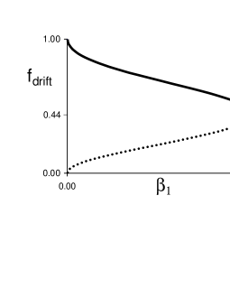
Figure 3: Fraction of oscillators in the chimera state that drift. Solid line, stable chimera; dotted line, unstable chimera.

Unfortunately, when the variables are plotted versus $\beta_{1}$, much of the bifurcation structure is hidden. In particular, two crucial events in the genesis of the chimera state occur when $f_{\textrm{drift}}=1$, $\beta_{1}=0$, and therefore collapse onto a single point in Figure 3. These events create the $x$-dependence in the chimera state, first in its local coherence $R(x)$ and then in its local average phase $\Theta(x)$. To see how such spatial structure arises, it is best to treat $\delta$, not $\beta_{1}$, as the relevant parameter, even though it is not a true control parameter (its turning points do not signify bifurcations, for example).

Figure 4 plots $u(\delta)$ vs. $\delta$ for the roots of Eq. (17). Branches have been coded with different dashing styles to indicate that they represent qualitatively different states. The zero branch along the $\delta$-axis, shown as a solid line, represents a family of spatially uniform drift states where both $R$ and $\Theta$ are independent of $x$. Such states occur only when $\beta=0$. They correspond to the exact (non-perturbative) solutions of Eq. (5) given by $\Theta(x)\equiv 0$ and $R(x)\equiv R=\sqrt{2\Delta-1}$, with $\frac{1}{2}\leq\Delta<1$. Linearization shows that this uniform drift state undergoes a zero-eigenvalue bifurcation at $\Delta=\frac{1}{2}(2+\epsilon)^{-2}$, valid for all $0<\epsilon<1$, implying a critical value of $\delta=\frac{1}{8}$ as $\epsilon\rightarrow 0$.

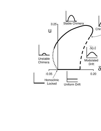
Figure 4: Solutions of Eq. (17) in $(\delta,u)$ plane, where $\delta=\Delta_{2}-c_{2}$ and $u=a_{2r}$. Inset panels show typical mean drift frequencies $\overline{\Delta}(x)$ in different regions of solution space. Panels with arrows indicate the shape of $\overline{\Delta}(x)$ for transitional values of $(\delta,u)$.

This is the first crucial event. At $\delta=\frac{1}{8}$, a spatially modulated drift state is born. Now $R$ depends on $x$. In perturbative variables, a root with $u=a_{2r}\neq 0$ bifurcates off the zero branch (shown dashed in Figure 4). Meanwhile, $a_{2i}=0$, so we still have $\Theta(x)\equiv 0$ for all $x$ (from Eq. (11) and $c_{i}=0$). Thus for states on the dashed branch, all the oscillators are drifting, and maintain the same average phase, but with different amounts of coherence at different values of $x$. Like the uniform drift states, these modulated drift states occur only if $\beta=0$.

The second crucial event occurs when the dashed branch intersects the line $u=\delta$. Then several things happen. The first locked oscillators are born; $a_{2i}$ and $\beta_{1}$ become nonzero; $\Theta$ depends on $x$; and a stable chimera is created. Evaluating the integral in (17) for $u=\delta$ shows that $\delta=16/9\pi^{2}\approx 0.18$ at the birth of the chimera.

Another way to distinguish among the various states is shown in the insets of Figure 4. For selected values of $\delta$ we have plotted the time-averaged frequency $\overline{\Delta}(x)$ of the oscillator at $x$, measured relative to the rotating frame. For locked oscillators, $\overline{\Delta}(x)=0$; for drifting ones, $\overline{\Delta}(x)=\sqrt{\Delta^{2}-R^{2}(x)}\sim\epsilon\sqrt{\delta-u\cos x}$, to leading order in $\epsilon$. Starting from the origin of Figure 4 and moving counterclockwise around the kidney bean, the corresponding graph of $\overline{\Delta}(x)$ is zero for the homoclinic locked state; flat for uniform drift states; modulated and positive for modulated drift states; and partially zero/partially nonzero for chimera states, with the fraction of drifting oscillators decreasing steadily as we circulate back toward the origin.

Although we have focused on the chimera state in Eq. (1), it also arises in other spatially extended systems. Indeed, it was first seen in simulations of the complex Ginzburg-Landau equation with nonlocal coupling Kuramoto and Battogtokh (2002); Kuramoto (2003). That equation in turn can be derived from a wide class of reaction-diffusion equations, under particular assumptions on the local kinetics and diffusion strength that render the effective coupling nonlocal Kuramoto and Battogtokh (2002); Kuramoto (2003); Shima and Kuramoto (2004); Tanaka and Kuramoto (2003).

In two dimensions, the coexistence of locked and drifting oscillators manifests itself as an unprecedented, bizarre kind of spiral wave—one without a phase singularity at its center Kuramoto (2003); Shima and Kuramoto (2004). Perhaps our analysis of its one-dimensional counterpart can be extended to shed light on this remarkable new mechanism of pattern formation.