Stable propagation of pulsed beams
in Kerr focusing media with modulated dispersion

Abstract

We propose the modulation of dispersion to prevent collapse of planar pulsed beams which propagate in Kerr-type self-focusing optical media. As a result, we find a new type of two-dimensional spatio-temporal solitons stabilized by dispersion management. We have studied the existence and properties of these solitary waves both analytically and numerically. We show that the adequate choice of the modulation parameters optimizes the stabilization of the pulse.

The analysis of the propagation of high power pulsed laser beams is among the most active fields of study in Nonlinear Optics, where the main dynamics phenomenon is the dependence of the refractive index of the materials with the amplitude of light fields. For propagation in materials showing a linear dependence of the refractive index with the laser intensity, the mathematical formulation of the beam dynamics is adequately described by the cubic nonlinear Schrödinger equation (NLSE) libros . In this case, the excitation of optical solitons is one of the most significant phenomena solitons .

Despite the success of the concept of soliton, these structures mostly arise in 1+1-dimensional configurations. This is mainly due to the well known collapse property of the cubic NLSE in multi-dimensional scenarios. This implies that a two-dimensional laser beam which propagates in a Kerr-type nonlinear medium, will be strongly self-focused to a singularity if the power exceeds a threshold critical value, whereas for lower powers it will spread as it propagates. Since collapse prevents the stability of multidimensional “soliton bullets” in systems ruled by the cubic NLSE, a great effort has been devoted to search for systems with stable solitary waves in multidimensional configurations bullets . It has been recently shown that a modulation of the nonlinearity along the propagation direction in the optical material can be used to prevent the collapse of two-dimensional laser beams Berge . The concept has been extended to the case of several incoherent optical beams Montesinos04 and to the case of matter waves siempre .

In this paper we use a similar idea to stabilize against collapse pulsed laser beams propagating in planar waveguides. This configuration is of great importance, as it is the common experimental procedure used for exciting spatial optical solitons. Instead of making a modulation of the nonlinearity our idea is to act on the chromatic dispersion term of the NLSE. Thus, our procedure resembles that used to obtain dispersion-managed temporal solitons in optical fibers.

We consider the paraxial propagation along $z$ of a pulsed beam of finite size in time $t$ and spatially confined by a waveguide along the $y$-axis. Thus, diffraction only acts in the $x$ direction and is balanced by the self-focusing nonlinearity given by a refractive index of the form: $n=n_{0}+n_{2}|\vec{E}|^{2}$. The dynamics of the slowly-varying amplitude of the pulse $\vec{E}$ is described by a 1+2D NLSE of the form:

$$2i\left(\frac{\partial\vec{E}}{\partial z}+k^{\prime}_{0}\frac{\partial\vec{E}}{\partial t}\right)+k^{\prime\prime}_{0}\frac{\partial^{2}\vec{E}}{\partial t^{2}}+\frac{1}{k_{0}}\frac{\partial^{2}\vec{E}}{\partial x^{2}}+2k_{0}\frac{n_{2}}{n_{0}}|\vec{E}|^{2}\vec{E}=0,$$ (1)

where $k_{0},k^{\prime}_{0}$ and $k^{\prime\prime}_{0}$ are respectively the wavenumber in vacuum, the inverse of the group velocity, and the group velocity dispersion coefficient.

As we mentioned above, for continuous beams an adequate modulation of $n_{2}$ along $z$ prevents collapse of the light distribution and yields to stabilized two-dimensional solitons. From a mathematical point ow view an equivalent effect can be achieved by suitably modifying the second order derivatives of the propagation equation Abd . However, it is physically impossible to change the sign of diffraction of a continuous beam during its evolution. Nevertheless, for the case of pulses, the temporal derivative in Eq. (1) can be modulated by changing the dispersion parameter $k_{0}^{\prime\prime}$, which can take positive as well as negative values. In this paper we will show that it is possible to stabilize a pulsed beam against collapse by modulating only the dispersion during beam propagation, without altering diffraction.

For a linearly polarized Gaussian pulsed beam with power $P=\int|E|^{2}dzdx$, an initial beam waist $w_{0,x}$ and temporal width $w_{0,t}$, it is useful to write the above Eq. (1) in adimensional form by means of the Fresnel length $F=k_{0}w_{0,x}^{2}$ in the “reduced time” frame. Thus, we make the rescaling: $\tau=(t-k^{\prime}_{0}z)/w_{0,t}$, $\eta=z/F$, $\chi=x/(F/k_{0})^{1/2}$ and $u=(w_{0,x}w_{0,t}/k_{0}^{\prime})^{1/2}E/P^{1/2}$. Then, if we consider that dispersion is modulated by a periodic function along propagation, we will finally yield to a generalized NLSE of the following form:

$$i\frac{\partial u}{\partial\eta}+\frac{1}{2}d(\eta)\frac{\partial^{2}u}{\partial\tau^{2}}+\frac{1}{2}\frac{\partial^{2}u}{\partial\chi^{2}}+g|u|^{2}u=0.$$ (2)

Here, $d(\eta)=Fk_{0}^{\prime\prime}/w_{0,t}^{2}$ and $g=k_{0}n_{2}PFk_{0}^{\prime}/n_{0}w_{0,x}w_{0,t}$. It is not obvious what kind of periodic function $g(\eta)$ will be more adequate to stabilize pulsed beams. A simple choice (and very natural for applications) is to take $d(\eta)$ as a piecewise constant function of the form $d(\eta)=d_{a}$ for $\eta\leq 2\eta_{a}$ and $d(\eta)=d_{b}$ for $2\eta_{a}<\eta\leq 2\eta_{b}$ (see top of Fig. 1) where $d_{a}$, $d_{b}$, $\eta_{a}$ and $\eta_{b}$ are free parameters that can be varied in order to fit experimental requirements and to optimize the stabilization of the pulsed beam.

To get some insight on the dynamics given by Eq. (2), we have performed an analytic study by means of the time-dependent variational approach Anderson . Notice that Eq. (2) can be obtained from the Lagrangian density:

$$2\mathcal{L}=i\left(u\dot{u}^{\ast}-u^{\ast}\dot{u}\right)+d(\eta)\left|\frac{\partial u}{\partial\tau}\right|^{2}+\left|\frac{\partial u}{\partial\chi}\right|^{2}-g\left|u\right|^{4},$$ (3)

where dots denote derivative with respect to $\eta$. We choose a Gaussian ansatz of the form:

$$u=A\exp\left[-\left(\frac{\chi^{2}}{2w_{\chi}^{2}}+\frac{\tau^{2}}{2w_{\tau}^{2}}\right)+i\left(\beta_{\chi}\chi^{2}+\beta_{\tau}\tau^{2}\right)\right].$$ (4)

The $\eta-$dependent parameters in the above equation have the following meaning: $A$ is the amplitude, $w_{\chi},w_{\tau}$ are the spatial and temporal widths and $\beta_{\chi},\beta_{\tau}$ are the initial curvature and chirp. Although Gaussians are not exact solutions of Eq. (2), our choice simplifies the calculations and is a usual lithg distribution in experiments. The standard variational calculations Anderson lead to the equations describing the dynamics of the pulsed beam spatial and temporal widths:

$$\ddot{w}_{\chi} = \frac{1}{w_{\chi}^{3}}-\frac{1}{2\pi}\frac{g}{w_{\chi}^{2}w_{\tau}},$$ (5a)

$$\ddot{w}_{\tau} = \frac{d(\eta)}{w_{\tau}^{3}}-\frac{1}{2\pi}\frac{g}{w_{\tau}^{2}w_{\chi}},$$ (5b)

Numerical simulations of Eqs. (5) show that the beam can be stabilized for many choices of the model parameters. These equations also predict two types of oscillations for width $w_{\tau}$: a fast one due to the modulation of dispersion and a slow one which almost coincides with the variation of $w_{\chi}$. This low frequency oscillation is generated by the internal nonlinear dynamics of the system.

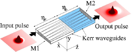
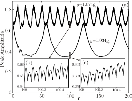
Figure 1: Top: Sketch of the propagation of a pulsed beam through a system with periodic modulation of dispersion made by joining two different planar Kerr waveguides. The forward-backward trajectory can be obtained by reflection at mirrors M1 and M2. Bottom: oscillations of the peak amplitude of stabilized pulsed beams propagating in the above system. In (a) the upper curve corresponds to a value $g=1.074g_{c}$ (surface plots in top figure). For the lower curve $g=1.034g_{c}$. The modulation is of the form: $d_{a}=1+8$, $d_{b}=1-8$, $2\eta_{a}=2\eta_{b}=0.04$. In (b) and (c) details of the fast oscillations are shown.

Variational models usually provide only simple and intuitive predictions that must be complemented with the integration of Eq. (2). All the results to be presented in this paper are based on direct simulations of Eq. (2) using a split-step Fourier method on a $520\times 520$ grid and absorbing boundary conditions to get rid of radiation. In Fig. 1 we plot the evolution of the peak amplitude of two different pulsed beams in a system sketched in Fig. 1 (top). In Fig. 1(a) the upper curve corresponds to a value $g=1.074g_{c}$, being $g_{c}>0$ the critical value of the nonlinearity for collapse. For the lower curve $g=1.034g_{c}$. The modulation is of the form: $d_{a}=1+8$, $d_{b}=1-8$, $2\eta_{a}=2\eta_{b}=0.04$. In (b) and (c) details of the fast oscillations are shown.

In Fig. 2 we plot the width oscillations of the stabilized soliton from Fig. 1 with $g=1.074g_{c}$. As the variational equations predict, the spatial width only displays a low frequency oscillation, whereas the temporal width presents small amplitude fast variations over the same low frequency main oscillation. This is clearly seen in the frequency spectra displayed in Fig. 2(d) and Fig. 2(e).

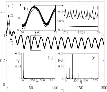
Figure 2: (a) Oscillations of the spatial (lower) and temporal (upper) widths of the stabilized soliton with $g=1.074g_{c}$ from Fig. 1(a). Insets (b) and (c) display details of the curves. Insets (d) and (e) show the frequency spectra of the spatial and temporal width oscillations, respectively.

In Fig. 3 we plot the results of simulation of Eq. (2) for the same input pulsed beams of Fig. 1. Now we take waveguides of half size, resulting in a frequency of modulation which is twice that of Fig. 1. Stabilization of both beams is achieved, showing the robustness of this idea.

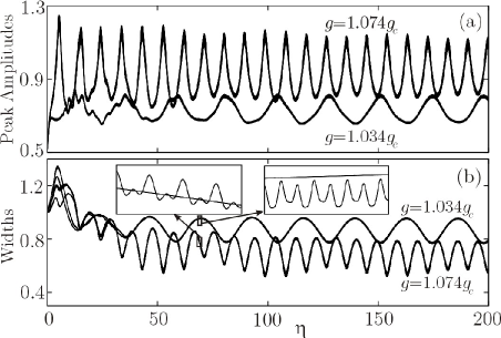
Figure 3: Oscillations of the peak amplitudes (a) and widths (b) of the same input solitons from Fig. 1. In this case the modulation is given by $d_{a}=1+8$, $d_{b}=1-8$, $2\eta_{a}=2\eta_{b}=0.02$. In (b) the oscillations of the spatial and temporal widths are overlapped (insets).

As a conclusion we can say that in this paper we have described two-dimensional spatio-temporal solitons which are stabilized against collapse by means of dispersion management. We have studied their stability and properties both analytically and numerically. We have shown that the adequate choice of the modulation parameters will optimize the stabilization of the pulse. Our results are of importance in the field of high power pulse propagation in nonlinear optical materials.

A remaining open question concerns the stability of higher-dimensional beams. In fact, at the present time it is not clear the mechanism of stabilization of fully three dimensional solitons which have been predicted to collapse in the case of modulation of nonlinearity siempre . Thus, our results on dispersion management would be an important step forward in stabilization of light bullets.

G. D. M. and V. M. P-G. are partially supported by Ministerio de Educación y Ciencia under grant BFM2003-02832 and Consejería de Educación y Ciencia of the Junta de Comunidades de Castilla-La Mancha under grant PAC-02-002. G. D. M. acknowledges support from grant AP2001-0535 from MECD.

References

- (1) C. Sulem and P. Sulem, The nonlinear Schrödinger equation: Self-focusing and wave collapse, (Springer, Berlin, 2000); Yu. S. Kivshar and G. P. Agrawal, Optical Solitons: From Fibers to Photonic Crystals, (Academic Press, San Diego, 2003).
- (2) V. E. Zakharov and A. B. Shabat, Sov. Phys. JETP. 34, 62 (1972); A. Hasegawa and F. Tapper, Appl. Phys. Lett. 23, 142-144 (1973); S. Maneuf, A. Barthelemy and C. Froehly, J. Optics. 17, 139-145 (1986).
- (3) See e.g. F. Wise and P. Di Trapani, Opt. Photonics News 13(2), 28 (2002); M. Segev and G.I. Stegeman, Phys. Today 51, No. 8, 42 (1998); H. Michinel, R. de la Fuente, J. Linares, Appl. Opt. 33, 3384-3390 (1994).
- (4) L. Berge, V. K. Mezentsev, J. J. Rasmussen, P. L. Christiansen and Y. B. Gaididei, Opt. Lett. 25, 1037 (2000); I.Towers and B.A.Malomed, J. Opt. Soc. Am. B 19, 537 (2002).
- (5) G. D. Montesinos, V. M. Pérez-García and H. Michinel, Phys. Rev. Lett. 92, 133901-1 (2004).
- (6) H. Saito and M. Ueda, Phys. Rev. Lett. 90, 040403 (2003); F. Abdullaev, J. G. Caputo, R. A. Kraenkel, and B. A. Malomed, Phys. Rev. A 67, 013605 (2003); G. D. Montesinos, V. M. Pérez-García and P. Torres, Physica D 191, 193-210 (2004).
- (7) F. Adbullaev, B. Baizakov, and M Salerno, Phys. Rev. E 68, 066605 (2003).
- (8) D. Anderson and M. Lisak, Phys. Rev. A 32 2270 (1985).