Square vortex solitons with a large angular momentum

Abstract

We show the existence of square shaped optical vortices with a large value of the angular momentum hosted in finite size laser beams which propagate in nonlinear media with a cubic-quintic nonlinearity. The light profiles take the form of rings with sharp boundaries and variable sizes depending on the power carried. Our stability analysis shows that these light distributions remain stable when propagate, probably for unlimited values of the angular momentum, provided the hosting beam is wide enough. This happens if the peak amplitude approaches a critical value which only depends on the nonlinear refractive index of the material. A variational approach allows us to calculate the main parameters involved. Our results add extra support to the concept of surface tension of light beams that can be considered as a trace of the existence of a liquid of light.

I Introduction

In wave mechanics, a vortex is a screw phase dislocation, or defect nye74 where the amplitude of the field vanishes. The phase around the singularity has an integer number of windings, $l$, which plays the role of an angular momentum. For fields with non-vanishing boundary conditions, this number is a conserved quantity and governs the interactions between vortices as if they were endowed with electrostatic chargesrozas97 . Thus, $l$ is usually called the “topological charge” of the defect.

Vortices are present in very different branches of physics like fluid mechanics, superconductivity, Bose-Einstein condensation, astrophysics or laser dynamics, among otherspismen99 . In Optics, a vortex with charge $l$ takes the form of a black spot surrounded by a light distribution. Around the dark hole, the phase varies from zero to $2\pi l$. These defects appear spontaneously in light propagation through turbulent media and can also be produced by appropriately shining a computer generated hologramheckenberg92 . The trace of vortices in a light field is a characteristic “fork-pattern” interferogram produced by superposition with a tilted planar wave.

The first experimental works on optical wavefront dislocations were carried out in the 80’s, in the context of adaptive systems, where phase singularities were a severe problem for image reconstruction techniquesbaranova8 . Later on they have been studied, among other fields, in optical tweezingsimpson97 , particle trappinggahagan96 , laser cavitiesweiss99 , optical interconnectorsscheuer99 or even to perform N-bit quantum computersmair01 .

Concerning light vortices in the nonlinear regimekivshar01 , the first theoretical work analysed their stability in Gaussian-like distributions propagating in optical Kerr materialskruglov85 . It was found for a cubic self-focusing refractive index, that a beam of finite size will always filament under the action of a phase dislocation. This also applies to saturable self-focusing nonlinearitiesfirth97 . On the other hand, vortex states were predicted and found experimentally for self-defocussing materials both in the Kerr case for continuous backgroundswartzlander92 and in the saturable case with finite size beamstikhonenko96 .

It was shown in quiroga97 that stable vortex states with $l=1$ can be obtained as stationary states of the propagation of a laser beam through cubic-quintic optical materialspiekara97 ; josserand97 ; davydova04 . This kind of nonlinearity is characterized by the $\chi^{(3)}>0$ and $\chi^{(5)}<0$ components of the nonlinear optical susceptibility and changes from self-focusing to self-defocusing at a given intensityfang02 . It has been recently shown that a gas-liquid phase transition takes place in light beams propagating in this type of materialsmichinel02 .

In this work, we will show that stable vortex states with a huge value of the angular momentum exist and their peak amplitude and propagation constant tend asymptotically, as the beam flux is increased, to values that do not depend on $l$. In this way, our results are in contradiction with previous worktowers01 , where it was claimed that stable vortex states in finite size beams exist only for the values $l=1,2$. For $l=3$ it was found a persistent weak instability which was also supposed to exist for higher values of the angular momentum.

In next section we will analyze the cubic-quintic nonlinear model, finding numerically the stationary states for a wide range of the angular momentum $l$ (up to 50) and describing their particular properties. Then, we will calculate analytically, by means of the variational method, the critical values of the propagation constant and peak amplitude that characterize the domain of existence of vortices. Finally, we will perform an azimuthal stability analysis to determine the domain zone where stable states can be found.

II The model

Let us start by writing the equation for laser beam propagation along $z$ in an optical cubic-quintic material. For paraxial propagation, the equation for the beam envelope $\Psi$ is a nonlinear Schrödinger equation (NLSE) of the form:

$$i\frac{\partial\Psi}{\partial z}+\nabla_{\perp}^{2}\Psi+\left(n_{2}|\Psi|^{2}-n_{4}|\Psi|^{4}\right)\Psi=0,$$ (1)

where $\nabla^{2}_{\perp}=r^{-2}\partial^{2}/\partial\phi^{2}+r^{-1}\partial/\partial r+\partial^{2}/\partial r^{2}$ is the transverse Laplacian operator in cylindrical coordinates $(r,\phi,z)$. The real positive constants $n_{2}$ and $n_{4}$ are given respectively by the $\chi^{(3)}>0$ and $\chi^{(5)}<0$ components of the nonlinear optical susceptibility and characterize the dependence of the refractive index on the intensity of the beam. If $n_{4}\leq 0$, a Gaussian beam of high enough power will undergo collapse after self-focusingchiao64 . The effect of a negative fifth order susceptibility ($-n_{4}$ term) combined with diffraction will stop the collapsing tendency for high powers, yielding to a stable two-dimensional condensed state of light with surface tension properties similar to those of usual liquidspiekara97 ; josserand97 ; michinel02 .

Figure 1: Numerically calculated radial amplitude profiles of the stationary states of Eq. (3) for $l=3$, 4, 10 and 50 with $\beta/\beta_{cr}$=0.1, 0.5, 0.9 and 0.99. In all the cases $n_{2}=n_{4}=1$ .

We are interested in stationary states with radial symmetry and angular momentum $l$ of the form:

$$\Psi(r,\phi,z)=\psi(r)e^{il\phi}e^{i\beta z},$$ (2)

where $\beta$ is the nonlinear phase shift or propagation constant and $\psi(r)$ is the radial envelope of the field. After substitution of (2) in (1), the following $z$-independent equation is obtained for $\psi(r)$:

$$-\beta\psi+\nabla_{r}^{2}\psi-\frac{l^{2}}{r^{2}}\psi+n_{2}\psi^{3}-n_{4}\psi^{5}=0,$$ (3)

where $\nabla^{2}_{r}\equiv\partial^{2}/\partial r^{2}+(1/r)\partial/\partial r$, is the radial part of the Laplace operator.

For a given integer value of $l$, a continuum of eigenstates with $\psi\rightarrow 0$ as $r\rightarrow\infty$ can be obtained by solving numerically Eq.(3). Close to the origin the shapes follow the linear regime with $\psi\propto r^{l}$. To this aim, we have used a standard relaxation technique. The profiles of the eigenstates for several values of $l$ and $\beta$ are plotted in Fig. 1 for the case of $n_{2}=n_{4}=1$. We particularly show states with $l=3$ and $l=4$ since these were previously found unstable in previous worktowers01 , as well as two examples of large angular momentum states ($l=10$ and $l=50$). In all cases, the stationary states can only be found for values of $\beta$ between zero and a fixed critical value $\beta_{cr}$quiroga97 , which does not depend on $l$.

It can be appreciated in the graphs that values of $\beta$ below $0.5\beta_{cr}$ yield to light distributions with smooth and wide Gaussian-like shapes. As $\beta$ is incremented the beam flux grows and the spatial profiles narrow, yielding to a minimum thickness of the ring of the stationary state for values of $\beta$ around $0.8\beta_{cr}$, keeping approximately the Gaussian shape. For larger values of the propagation constant, the beam flux grows rapidly with $\beta$ and the peak amplitude of the distribution saturates due to the effect of $n_{4}$, reaching asymptotically the value $A_{cr}$ which is slightly below the maximum amplitude. Thus, high power beams show spatial light distributions with flatted tops in their profiles, similar to those of hyper-Gaussian functionsdimitrievski99 ; quiroga99 .

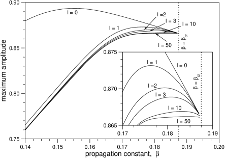
Figure 2: Maximum amplitude of the stationary states versus propagation constant for angular momenta $l$=0, 1, 2, 3, 10 and 50. All the curves join at the point $A=A_{cr}=0.866$, $\beta=\beta_{cr}=0.1875$. Inset: detail of the zone close to $\beta_{cr}$ where the calculations become delicate.

We must stress the intriguing fact that both $\beta_{cr}$ and $A_{cr}$ do not depend on the value of the topological charge. This is shown in Fig. 2, where the maximum amplitude has been plotted as a function of $\beta$. In the inset, the zone $\beta\approx\beta_{cr}$ can be seen in detail. As can be appreciated, whatever the value of $l$ is, all the curves tend to join at the same point. This means that the critical value of the propagation constant and peak amplitude only depend on the nonlinearity and not on the angular momentum. We will revise this result in our analytical study of the next section.

It also worths to mention that the central hole increases its size with the topological charge for a fixed value of $\beta$, as can be seen comparing the profiles in Fig. 1 for $l=3,4$ with $l=10,\,50$. This is also clearly shown in Fig 3, where we plot several eigenstates with values of the angular momentum ranging from $l=1$ up to $l=9$, with propagation constant $\beta=0.95\beta_{cr}$. Besides, if $\beta$ grows, the radius of the hole increases. As the value of $\beta$ approaches $\beta_{cr}$ the thickness of the external ring grows faster than the internal hole, and the final result takes the asymptotic form of a dark spot surrounded by a larger ring of light of almost constant shape which ends abruptly at a given radius. This behavior can be assessed having a look to Fig.4, where the dimensions of the internal hole and the ring thickness are plotted versus the propagation constant for the particular case of $l=10$. A logarithmic scale was chosen to highlight that the growth in the ring thickness clearly dominates over the hole radius from certain value of the propagation constant. In the inset it is also shown, as an example, one of the stationary states with $\beta$ very close to $\beta_{cr}$, showing the huge ring whose width clearly exceeds the hole radius and presents a practically rectangular shape.

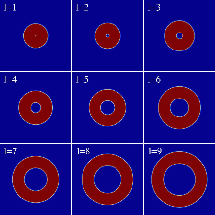
Figure 3: (Color on line) Azimuthal eigenstates of Eq.(2) for $l=1$ to $9$ with $\beta=0.95\beta_{cr}$.

Figure 4: Dependence of the internal hole radius (continuous line) and ring thickness (dashed line) with the propagation constant $\beta$ in the vicinity of $\beta_{cr}$ for eigenstates with $l=10$. Inset: example of a stationary state with $l=10$ and $\beta=0.9998\beta_{cr}$.

III Variational analysis

To explain the properties of the above light distributions, we have performed a variational analysisdimitrievski99 ; quiroga99 . It is easy to demonstrate that the stationary system described by the model (3) can be obtained from the following Lagrangian function:

$$\mathcal{L}=r\left\{\left(\frac{d\psi}{dr}\right)^{2}+\left(\frac{l^{2}}{r^{2}}-\beta\right)\psi^{2}-\frac{n_{2}}{2}\psi^{4}-\frac{n_{4}}{3}\psi^{6}\right\}.$$ (4)

Now assuming a rectangular shape of the stationary states for values of $\beta$ close to $\beta_{cr}$ (see Fig. 1), we choose a trial function $\psi_{v}(r)$ centered at $r_{0}$ with amplitude $A$ and width $2w$, given by:

$$\psi_{v}(r)=\left\{\begin{array}[]{ll}A,&|r-r_{0}|\leq w\\ 0,&|r-r_{0}|>w\end{array}\right.$$ (7)

Thus, $r_{0}$, $A$ and $w$ are the variational parameters. Using this trial function and minimizing the average over the Lagrangian $<\mathcal{L}>$ respect to each parameteranderson83 , we obtain the following conditions:

$$\frac{l^{2}}{r_{0}^{2}-w^{2}}+\frac{n_{2}}{2}A^{2}-\frac{n^{4}}{3}A^{4}-\beta=0,$$ (8)

$$\frac{l^{2}}{2r_{0}w}\ln\left(\frac{r_{0}+w}{r_{0}-w}\right)-n_{2}A^{2}-n_{4}A^{4}+\beta=0.$$ (9)

where Eq. (8) is obtained from the minimization respect to $r_{0}$ and $w$ (the same condition is obtained for both parameters), and Eq. (9) follows from minimization respect to parameter $A$. In the limit when $\beta\rightarrow\beta_{cr}$, the first term of both equations vanishes. This follows by taking into account that $r_{0}>w$ should always be satisfied (otherwise there would be no hole), then we have $r_{0}^{2}-w^{2}>r_{0}^{2}\rightarrow\infty$ and $(r_{0}^{2}-w^{2})^{-1}\rightarrow 0$, consequently the first term of Eq. (8) is zero. For Eq. (9), the argument of the logarithm tends to infinity as it is easily deduced from the fact that the ring width grows faster than the hole radius and $r_{0}>w$ ($(r_{0}+w)/(r_{0}-w)>2w/(r_{0}-w)\rightarrow\infty$). However, this term diverges logarithmically, meanwhile the denominator goes to infinity quadratically (product $r_{0}w$), and consequently the whole term tends to zero. Finally, we can solve them for $A_{cr}$ and $\beta_{cr}$ to obtain:

$$A_{cr}={\left(\frac{3n_{2}}{4n_{4}}\right)}^{1/2},$$ (10)

$$\beta_{cr}=\frac{3n_{2}^{2}}{16n_{4}}.$$ (11)

For the particular case considered in the numerical calculations displayed in Figs. 1-2, i.e. taken $n_{2}=n_{4}=1$, the values obtained for the critical parameters are $A_{cr}=0.866025$ and $\beta_{cr}=0.1875$. The comparison of these analytical results with the numerical calculations shows an excellent agreement, since both values are exactly those guessed numerically (see Fig. 2). This so good result is due to the choice of the trial function, which fits almost exactly with the numerical solution for values close to the critical point.

IV Stability analysis

In order to test the stability of the stationary states we calculated the growth rates of small azimuthal perturbations to find out the value of $\beta$ at which they vanish. Additionally, in order to assess the accuracy of the previous analysis, we propagated some unstable eigenstates with a split-step Fourier method and found their splitting distances. The inverse of these values should coincide, except for a constant scale factor, with the dominant perturbation eigenvalues calculated in the azimuthal instability analysis. Finally, we have also simulated other kind of perturbations like total reflection at the boundary between a cubic-quintic material and air. As we will see below, the eigenstates show robust behavior against these collisions and preserve their angular momentum although strong oscillations are observed.

To carry out the perturbation analysis, we add to the original eigenstate a small $p$-order azimuthal perturbation functionfirth97 ; soto91 :

$$\tilde{\Psi}(r,\phi,z)=[\psi(r)+f(r,z)e^{ip\phi}+h(r,z)e^{-ip\phi}]e^{i(l\phi+\beta z)},$$ (12)

where $f(r,z)$ and $h(r,z)$ are the small complex components of the eigenstate of the $p$-order azimuthal perturbation. Our interest is to seek those functions which grow exponentially with $z$, so we assume that they have the form:

$$f(r,z)=[f_{1}(r)+if_{2}(r)]e^{\delta_{p}z},$$ (13)

$$h(r,z)=[h_{1}(r)+ih_{2}(r)]e^{-\delta^{*}_{p}z},$$ (14)

being the parameter $\delta_{p}$ the perturbation eigenvalue. In this way, the real part of $\delta_{p}$ constitutes the growth rate of this perturbation. If we replace the perturbed eigenstate (Eq. (12)) into Eq. (1) and keep only the first order terms in $f(r,z)$ and $h(r,z)$ (linearisation) we obtain the following set of coupled differential equations for those components $f(r,z)$ and $h(r,z)$:

$$i\frac{\partial f}{\partial z}+\nabla^{2}_{r}f-\frac{(l+p)^{2}}{r^{2}}f+Q(\psi)f+R(\psi)h^{*}=0$$ (15)

$$i\frac{\partial h}{\partial z}+\nabla^{2}_{r}h-\frac{(l-p)^{2}}{r^{2}}h+Q(\psi)h+R(\psi)f^{*}=0,$$ (16)

where $Q(\psi)\equiv-\beta+(2n_{2}-3n_{4}|\psi|^{2})|\psi|^{2}$ and $R(\psi)\equiv(n_{2}-2n_{4}|\psi|^{2})|\psi|^{2}$. The solution of this equation system is obtained using a Crank-Nicholson scheme to propagate an initial arbitrary guess until the shape of each component does not change perceptiblysoto91 . According to the component dependence on $z$ (Eq. (13)), the value of the growth rate can be calculated at each propagation step by:

$$\mathrm{Re}\,\delta_{p}=\frac{1}{2\Delta z}\ln\frac{|f(r,z+\Delta z)|^{2}}{|f(r,z)|^{2}},$$ (17)

where $\Delta z$ is the propagation step and the function $f(r,z)$ is evaluated in a fixed point $r$, usually that which corresponds to the maximum. Besides, the functions can be rescaled at each step by this maximum value to avoid an overflow. The propagation is carried out until the value of the perturbation growth rate does not change any more, what indicates that convergence was reached. This allows us to obtain the growth rates $\mathrm{Re}(\delta_{p})$ for different order perturbations versus the propagation constant, as depicted in Fig. 5.

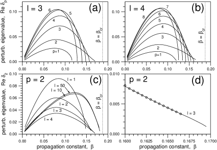
Figure 5: Growth rate of the azimuthal perturbation versus $\beta$. In (a) and (b), the angular momentum is fixed ($l=3$ for (a), $l=4$ for (b)) and the values of the perturbation order $p$ are indicated by labels near the curves. In (c) the growth rate for the perturbations with $p=2$ for $l=1$, 2, 3, 4, 10 and 50 are plotted. In (d), a comparison between the inverse of the splitting distance (dots) and $p=2$ perturbation eigenvalue for unstable states with $l=3$ is shown.

The growth rates for vortices with angular momentum $l=3$ and $l=4$ are shown in Figs. 5(a)-(b). As can be seen, all of them fall to zero for a value of $\beta$ below $\beta_{cr}$, what implies the existence of a stability window, in contradiction with previous calculations where all the states with $l>2$ where found unstabletowers01 . Our results show that the maximum growth rate corresponds to perturbation eigenvalues with $p\approx 2l$, what allows to estimate the number of filaments $N$ resulting from the breakup of the unstable vortices ($N\approx 2l$). Besides this, the perturbation $p=2$ has been proved to be the most persistent, despite the value of the angular momentum. Hence, in Fig. 5(c) we plot the curves associated to this perturbation for different values of the angular momentum, including the cases corresponding to $l=10$ and $l=50$. As can be appreciated in these plots, there exists a window between the vanishing point and the limit value for $\beta$ ($\beta=\beta_{cr}$), what proves the existence of a stability zone close to the critical point containing an infinite number of stable eigenstates. Note that this window narrows for high values of $l$ but remains finite. As $l$ increases, the point at which the perturbation vanishes approaches asymptotically the critical point. However, we believe that the critical point itself is never reached, even for arbitrarily high values of the topological charge.

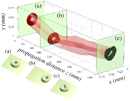
Figure 6: (Color on line) Numerical simulation of the total reflection at a planar boundary between a cubic-quintic and a linear media (air). For this stationary state the angular momentum is $l=4$ and the propagation constant $\beta=0.95\beta_{cr}$. The top image is an isosurface of the propagating beam. The boundary between the nonlinear material and air is the plane $y=0$. The images (a)-(c) correspond to different transversal cutoffs (intensity profiles) of the beam at different values of the propagation distance $z$.

When $\beta$ is close to $\beta_{cr}$ the azimuthal analysis turns itself very delicate and it has to be carried out in a very careful way. In fact, convergence takes a much longer distance and an erroneous final result is obtained if the number of samples and the propagation step are not chosen appropriately. In this sense, combining the analysis with direct calculations of the splitting distance of the unstable eigenstates is definitively useful. In Fig. 5(d) it is zoomed the region of 5(c) where the perturbation for $l=3$ drops to zero. The points obtained propagating the eigenstates and taking the inverse of the distance where they split are also plotted. These values were subsequently scaled by the same constant value to compare with the perturbation eigenvalue curve. As can be appreciated, the values obtained from this propagation experiments fall to zero with the same slope as the perturbation eigenvalues do. When the stability analysis is not performed with enough accuracy a more steady behavior of the curve appears, what implies that the eigenvalue falls to zero at a higher value of $\beta$. This allows us to assess the validity of the perturbation analysis.

As a final test of the stability of the eigenstates, we have simulated the total reflection at a planar boundary between a cubic-quintic material and air for beams with different angular momenta. For the simulation we have used a split-step Fourier method with a $520\times 520$ grid. The idea is similar to the test of surface tension properties of ”liquid light beams” from ref. michinel02 . As can be seen in Fig. 6, a beam with $l=4$ does not split after the total reflection, although a strong oscillation is observed. This is another proof of the stability of these nonlinear waves. We must notice that depending on the incidence angle, a strong deformation of the beam can be induced, which can yield to a split or a decay of the inner vortex into several defects with lower topological charges paz-alonso04 .

V Conclusions

The main conclusions that can be derived from the present work are the following: first, stable azimuthal finite-size beams with arbitrary very large angular momentum can exist in optical materials with self-focusing (cubic) and defocussing (quintic) nonlinearity. Second, the shapes of these beams tend asymptotically to square-like ring profiles with bigger dark holes for higher values of the angular momentum. And finally, the critical values of the propagation constant and amplitude do not depend on the angular momentum of the beam.

References

- (1) J. F. Nye and M. V. Berry, Proc. R. Soc. London A 336, 165-190 (1974).
- (2) D. Rozas, Z. S. Sacks, and G. Swartzlander Jr. , Phys. Rev. Lett. 79, 3399-3402 (1997).
- (3) L. Pismen, Vortices in nonlinear fields, (Oxford University Press, London, 1999).
- (4) N. R. Heckenberg, R. McDuff, C. P. Smith, and A. G. White, Opt. Lett. 17, 221-223 (1992).
- (5) N. B. Baranova, B. Ya. Zel’dovich, A. V. Mamaev, N. F. Pilipetslii, and V. V. Shkukov, Pis’ma Zh. Eksp. Teor. Fiz. 33, 206-209 (1981) [JETP Lett. 33, 195 (1981)];
- (6) N. B. Simpson, K. Dholakia, L. Allen, and M. J. Padgett, Opt. Lett 22, 52-54 (1997).
- (7) K. T. Gahagan and G. A. Swartzlander, Jr. , Opt. Lett. 21, 827 (1996).
- (8) C. O. Weiss, M. Vaupel, K. Staliunas, G. Slekys, and V. B Taranenko, Appl. Phys. B 68, 151-168 (1999).
- (9) J. Scheuer and M. Orenstein, Science 285, 230-233 (1999).
- (10) A. Mair, A. Vaziri, G. Weihs and A. Zeilinger, Nature 412, 313-316 (2001).
- (11) Yu. S. Kivshar and E. Ostrovskaya, Opt. Photon. News 12, 24-28 (2001).
- (12) V. I. Kruglov and R. A. Vlasov, Phys. Lett. A 111, 401-404 (1985).
- (13) W. J. Firth and D. V. Skryabin, Phys. Rev. Lett. 79, 2450 (1997).
- (14) G. A. Swartzlander, Jr. and C. T. Law, Phys. Rev. Lett. 69, 2503-2506 (1992).
- (15) V. Tikhonenko and N. Akhmediev, Opt. Commun. 126, 108-112 (1996).
- (16) M. Quiroga-Teixeiro and H. Michinel, J. Opt. Soc. Am. B 14, 2004 (1997).
- (17) A. H. Piekara, J. S. Moore, and M. S. Feld, Phys. Rev. A 9, 1403 (1974).
- (18) C. Josserand and S. Rica, Phys. Rev. Lett. 78, 1215 (1997).
- (19) T. A. Davydova and A. I. Yakimenko, J. Opt. A: Pure Appl. Opt. 6, S197-S201 (2004).
- (20) G. Fang, Y. Mo, Y. Song, Y. Wang, C. Li, and L. Song, Opt. Commun. 205, 337-341 (2002).
- (21) H. Michinel, J. Campo-Táboas, R. García-Fernández, J. R. Salgueiro, and M. Quiroga-Teixeiro, Phys. Rev. E 65, 066604-1-7 (2002).
- (22) I. Towers, A. V. Buryak, R. A. Samut, B. A. Malomed, L.C. Crasovan, and D. Mihalache, Phys. Lett. A 288, 292-298 (2001).
- (23) R. Y. Chiao, E. Garmire, and C. H. Townes, Phys. Rev. Lett. 13, 479 (1964).
- (24) K. Dimitrievski, E. Reimhult, E. Svensson, A. Öhgren, D. Anderson, A. Berntson, M. Lisak, and M. L. Quiroga-Teixeiro, Phys. Lett. A 248, 369 (1998).
- (25) M. Quiroga-Teixeiro, A. Berntson, and H. Michinel, J. Opt. Soc. Am. B 16, 1697 (1999).
- (26) D. Anderson, Phys. Rev. A 27, 3135-3145 (1983).
- (27) J. M. Soto-Crespo, D. R. Heatley, and E. M. Wright, Phys. Rev A 44, 636-644 (1991).
- (28) M. J. Paz-Alonso, D. Olivieri, H. Michinel, and J. R. Salgueiro, Phys. Rev. E69, 056601-1-6 (2004).