Localization in the Nonanalytic Quantum Kicked Systems

Abstract

Numerical investigations on nonanalytic quantum kicked systems is presented in this paper. The power-law type localization is found to be universal in the nonanalytic systems just like that the exponential type in the analytic systems. With increasing the perturbation strength, a transition from perturbative localization, to pseudo-integrable regime, to dynamical localization and to complete extension is clearly demonstrated. The different regimes are characterized by the different relations between the localization length and the system’s parameters. Finally, we investigate the diffusion behavior and find that the quantum suppression is relaxed in the nonanalytic systems.

I introduction

The quantum dynamics of classically chaotic Hamiltonian systems has attracted great interest in recent years. Much work has been devoted to study of the periodically ”kicked” systems. The prime examples are the kicked rotor (KR)casati1 ; casati2 and the kicked hydrogen atom three . In these models, an interesting phenomenon is the dynamical localization, namely, the quantum suppression of classical diffusion. This phenomenon was first discovered numerically by Casati et al casati1 in the KR model , and later on confirmed by several experiments such as Rydberg atom in microwave field four . The deviation from maximal chaos in quantum model is entirely related quantum interference effects only. It was shown that the mechanism of such a ”quantum suppression of classical chaos” is the localization of all eigenfunctions in the unperturbed momentum space, which similar to the well-known Anderson localization in the solid state physics.

However, these discussions are mainly restricted to the analytical systems. On the other hand, nonanalytic systems also emerge from the study of more concrete physical models, such as, Fermi-acceleration modelfcm , billiad system bs1 ; bs2 and a kicked particle in 1D infinite square potential wellblgh . Recently, some pioneering works have been done towards the systems in which the analyticity condition is broken down bbb1 ; bbb2 ; bbb3 . Many novel properties are found, such as the important role of the cantori structure in the localization. Their discussions are mainly towards a special discontinuous model, where the derivative of the potential is discontinuous.

The main purpose of this paper is to observe the quantum behavior, especially the localization phenomenon in the general nonanalytic systems. As will be seen later, the nonanalytic systems reveals distinctive properties. The power-law type localization is found to be universal, just like the exponential localization in analytic models. In particular, the power exponent does not relate to the derivative order of the potential. It rests on the convergence rate of the corresponding Fourier series. The localization length properly defined in light of the information entropy reveals four different regimes with increasing the perturbation strength: perturbative localization; pseudo-integrable regime; dynamical localization; complete extension. Each regime is characterized by different relation between the localization length and the system’s parameters. Moreover, we investigate the diffusion behavior and show that the suppression of the energy diffusion can be relaxed in the nonanalytic systems.

The paper is organized as follows. In Sec.II we introduce the nonanalytic Hamiltonian considered in the paper and discuss its classical diffusion property. The power-law type eigenstates is shown in Sec.III. In Sec.IV, we calculate the localization length defined in terms of the information entropy. The energy diffusion in nonanalytic systems is discussed in Sec.V. Finally, Sec.VI is the concluding remarks.

II Nonanalytic Models and Classical Dynamics

The considered Hamiltonian takes the form (in dimensionless units),

$$\hat{H}=\frac{\hat{p}^{2}}{2}+k\hat{V}(q)\delta_{T}(t),\,\delta_{T}(t)=\sum_{m=-\infty}^{+\infty}\delta(t-mT),$$ (1)

where the potential $V(q)$ is $2\pi$-periodic function, taking the following form under the Fourier expansion,

$$V(q)=\sum_{n=1}^{\infty}a_{n}\sin(nq)+b_{n}\cos(nq).$$ (2)

To simplify our discussions, let $a_{n}=\frac{1}{n^{\alpha}}$, $b_{n}=0$, then

$$V(q)=V_{\alpha}(q)=C_{\alpha}\sum_{n=1}^{\infty}\frac{\sin(nq)}{n^{\alpha}},$$ (3)

where the $C_{\alpha}$ is the normalizing constant so that the maximum value of the potential be unit. The parameter $\alpha$ represents the convergence rate of Fourier series. As $\alpha$ goes to infinity, only the first term of the series remains, which is just the sinusoidal function. In this case the system is equivalence to the KR model under a displacement transformation. The potential functions are plotted in Fig.1.

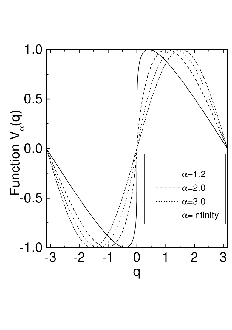
Figure 1: The nonanalytic potential functions $V_{\alpha}(q)$

Before we go further, let us discuss the symmetry problems of the system. Clearly the time-reversal invariance is kept for any $\alpha$. However, for $\alpha\neq\infty$, two essential modifications are made: 1) $V_{\alpha}(q)$ turns to be nonanalytic ($\in C^{(\beta)}$), the order of its derivability is $\beta=[\alpha]-2$, e.g. its $(\beta+1)$-order derivative diverges or discontinuous at $q=0$. Here $[x]$ represents the minimum integer larger than or equals to x; 2) Spatial symmetry is broken down, the parity is no longer a good quantum number. As shown later, these two changes will substantially alter the quantum properties of the system.

Classically, the Hamiltonian (1) corresponds to a twisted map,

$$p_{n+1}=p_{n}+k\frac{\partial{V_{\alpha}(q_{n})}}{\partial q_{n}},$$

$$q_{n+1}=q_{n}+Tp_{n+1}\,\,\,mod(2\pi).$$ (4)

The classical parameter $K=kT$ determines its classical dynamics. In our calculations we fix $T=1$. As $\alpha$ be an integer, the potential can be expressed analyticly, for example,

$$\frac{\partial{V_{\alpha}(q)}}{C_{\alpha}\partial q}=\left\{\begin{array}[]{ll}ln(2sin(q/2))&\alpha=2\\ \frac{1}{12}[(q^{2}-\pi q)+(2q-\pi)(q-2\pi)]&\alpha=3,q\in[0,2\pi).\\ \frac{1}{48}[q^{2}(q-2\pi)^{2}-\frac{8}{15}\pi^{4}]&\alpha=5\end{array}\right.$$ (5)

As well known, the KAM theorem is the footstone of modern dynamics theory. It states that invariant tori (KAM tori) of irrational winding number will keep up under a small perturbation whereas the tori corresponding to the rational winding number are broken down. Fortunately, the broken tori have zero-measure set in the phase plane. In the original proof of the theorem, the analyticity is strictly required. However, it is found later on that, the analyticity condition can be relaxed to $C^{(3+\epsilon)}$ herm for a twisted map. Applying this result into our system, it means that for $\alpha>6$, KAM theorem is available; As $\alpha\leq 6$, the system is non-KAM system.

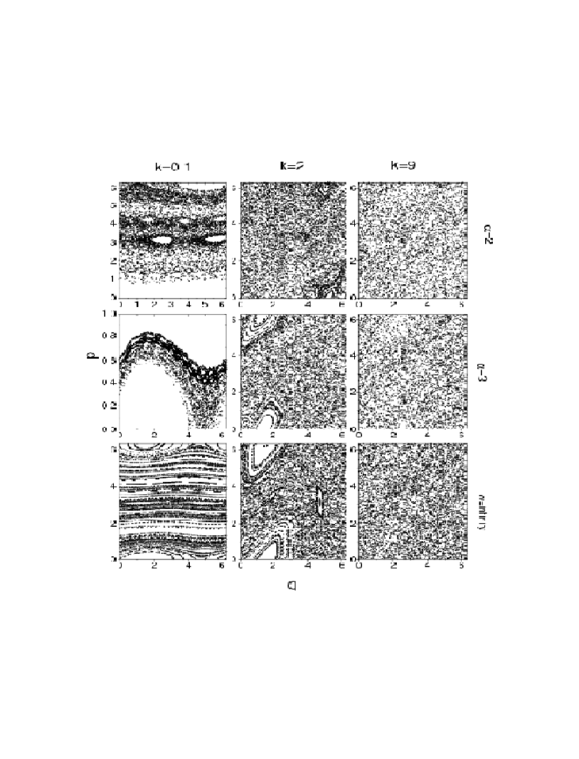
Figure 2: Local phase plane for various parameters. As $\alpha=2,3$ and $k=0.1$, the phase plane is ploted by tracing one trajectory originated from the stochastic region for ten thousands or more periods.

The main characteristic of the non-KAM system is the broken-up of the KAM tori under a small perturbation so that the diffusion can take place. In Fig.2, we plot the local phase planes of systems corresponding to $\alpha=2,3,\infty$. It is shown that phase plane become more and more chaotic as we increase the perturbation strength $K$. At small value of $K=0.1$, the phase plane of the nonanalytic systems show complicated structures, such as the stochastic webs and cantori. The chaotic region is connected and the diffusion can occur. As $K$ is larger than a critical value $K_{cr}$, the phase planes become fully chaotic, or ergodic. The critical values can be estimated approximatly from the losing stability of the primary resonances. Approximately, it gives $K_{cr}(\alpha=2)\simeq 3.5,K_{cr}(\alpha=3)\simeq 4.5,K_{cr}(\alpha=5)\simeq 4.6$ and $K_{cr}(\alpha=\infty)\simeq 5.2.$ In the intermediate perturbation $K=2$, even though the KAM tori are completely broken down, there are some invariant structures, such as small islands, cantori.

In calculating the diffusion coefficient for a given $K$, we take 1000 points starting from stochastic regions, and all the initial trajectories evolve for several thousand periods. Averages are taken over 1000 trajectories for each time period. It is found that the energy diffusion is asympotically linear for all values of $K$. The diffusion coefficient $D(\equiv<\Delta P_{n}^{2}>/n)$ (n is the time in unit of T) versus $K$ is plotted in Fig.3. As the $K$ is large enough i.e. $K>K_{cr}$, the diffusion coefficients show $D\simeq b_{\alpha}K^{2}$ in the quasilinear approximation, where $b_{\alpha}=0.843,0.550$ and $0.500$ for $\alpha$ be $2,3$ and $\infty$, respectively. In this case, the phase plane is fully chaotic. Below these threshold values, diffusion coefficients show various behavior for different $\alpha$. At $\alpha=2$, a scaling law like $D\sim K^{5/2}$ is obviously demonstrated. At $\alpha=3$, as $K<0.5$, $D\sim K^{2}$ and then a $D\sim K^{7/2}$ scaling law. At $\alpha=\infty$, as $K>1$ the diffusion coefficient abruptly rises to the quasi-linear approximation regime.

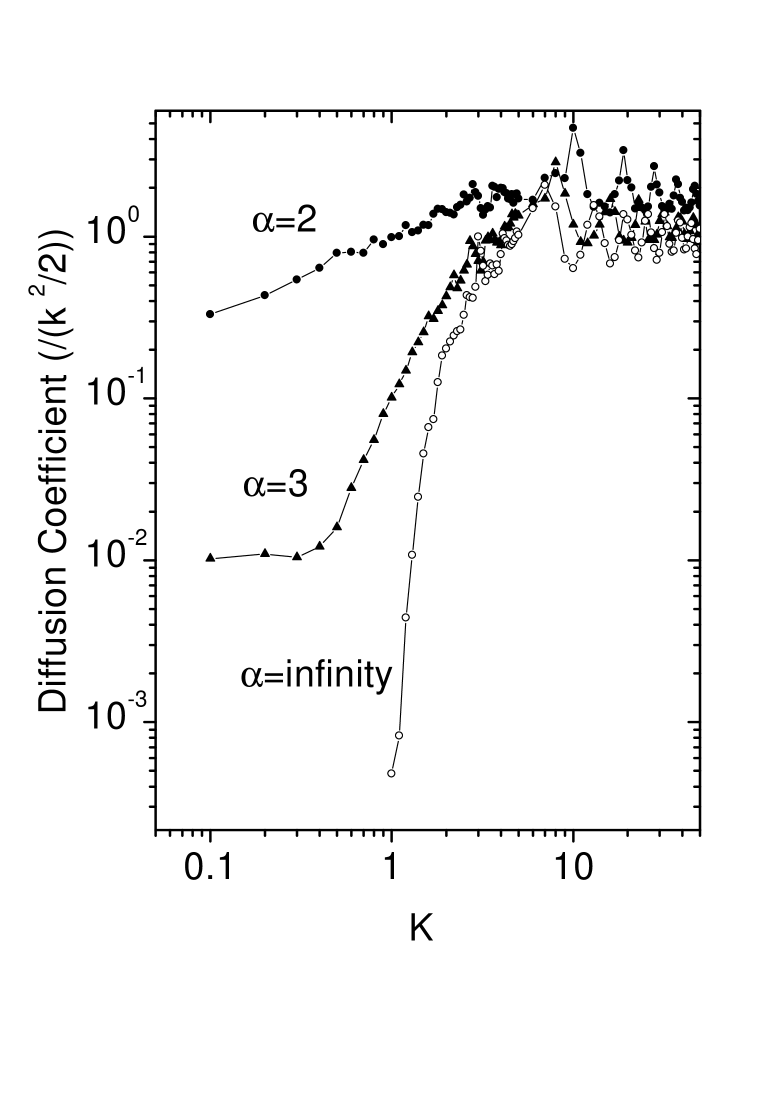
Figure 3: Classical diffusion coefficients versus the perturbation strength for various $\alpha$.

III Eigenstates

Now we turn to the quantum properties of the nonanalytic models and to see how the classical chaos manifests itself in the quantum dynamics. The evolution operator over the period $T$ of the kick is given by

$$\hat{U}(T)=exp(-\frac{i\hat{P}^{2}T}{4\hbar})exp(-\frac{ik\hat{V}_{\alpha}(q)}{\hbar})exp(-\frac{i\hat{P}^{2}T}{4\hbar}).$$ (6)

It is unitary and satisfies following eigenvalue equation, $\hat{U}(T)|\Phi_{\lambda}>=e^{-\frac{i\lambda}{\hbar}}|\Phi_{\lambda}>$; Here the eigenphase $\lambda$ is real, $\lambda/T$ is so called quasi-energy, $\Phi_{\lambda}$ is the eigenstate or Floquet state.

The Floquet states and the quasi-energy can be obtained by diagonalizing $\hat{U}(T)$ within a large number of plane wave bases $|n>,(n=-\frac{N}{2},...\frac{N}{2})$. In our calculations $N$ is kept at 1024 and $\hbar=T=1$. The elements of matrix are $U_{nm}=\langle n|\hat{U}(T)|m\rangle$. The fast Fourier transformation (FFT) is employed to transform the wave function between the position representation and momentum representation in our numerical calculations. Detailed description of the numerical method refer to blgh ; HLLZ .

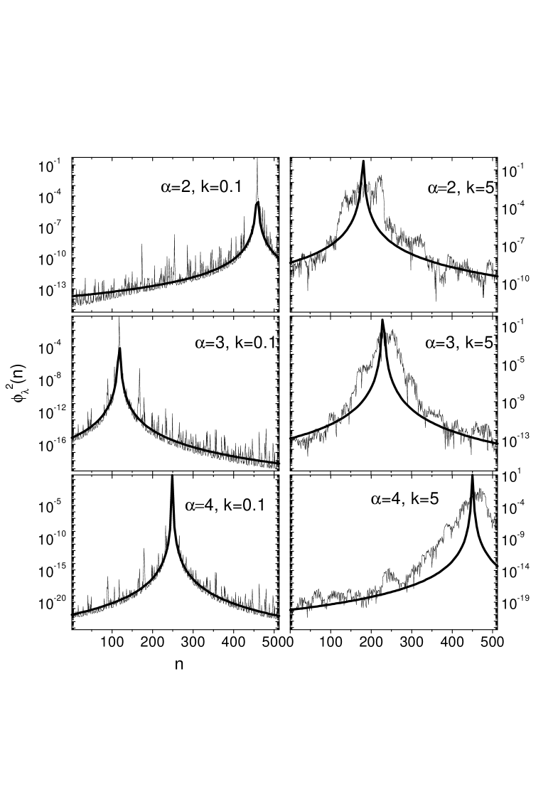
Figure 4: The typical eigenvectors in momentum representation for different parameters. The smooth curves represent the Lorentz-like distributions (Eq.8). The relation between power exponent and the parameter $\alpha$ is $\gamma=2\alpha$.

In the KR model, the eigenstates are always exponentially localized in the momentum space. For the nonanalytic systems, the things are quite different. The time-reversal invariance imposes certain condition on the eigenvector $\Phi_{\lambda}$, that is,

$$\Phi_{\lambda}(n)=e^{ia}\Phi_{\lambda}^{*}(-n),$$ (7)

with $a$ being a constant phase, independent of $n$. So in Fig.4, only the half number of the components in the momentum coordinates are plotted. We find that, for a small perturbation (k=0.1), i.e. in the perturbative regime, the envelope of Floquet states in momentum representation can be well fitted by Lorentz-like function (see left column of Fig.4):

$$|\Phi_{\lambda}(n)|^{2}\simeq\frac{c_{1}}{1+c_{2}|n-n_{c}|^{\gamma}}.$$ (8)

with $c_{1},c_{2}$ are the fitted constants.

The power-law localization is clearly demonstrated. In particular, the power exponent $\gamma$ does not relate to the $\beta$, the derivative order of the potential. It rests on the convergence rate of the corresponding Fourier series, i.e. a simple relation is given numerically,

$$\gamma=2\alpha.$$ (9)

With increasing the perturbation strength, the eigenstate shows a chaotic band whose width is proportional to $k$. Outside the band, the tails of eigenvector is found to decay, on average, as power-law. The relation between the power exponent and the index $\alpha$ expressed by Eq.(9) still holds (see right column of Fig.4).

In fact, the power-law type localization of the eigenstates can be traced back to the structure of the matrix $U$. In the KR model, the values of matrix elements $U_{mm+n}$ decay faster than exponential when $n$ exceeds the band width $b$ which is proportional to $k$, thus the elements outside this diagonal band can be safely regarded as zero. Within the band of width $b$, the elements are proved to be pseudorandomcasati2 . However, in our model the situation is different. Careful analysis yields that the elements outside the band decay as a power law with $|U_{m,m+n}|\sim 1/n^{\alpha}$. We have calculated $\langle U^{2}\rangle_{n}(\equiv\langle U^{2}_{m,m+n}\rangle$) (the average is done over $m$). The typical slope of the curves over a large range is approximately minus $2\alpha$ (see Fig.5). And the diagonal band width $b$ in our model is also found to be approximately proportional to $k$ (Fig.5b). This kind of band random matrix, describes a new class of physical system, e.g. nonanalytic system, has attracted recent attentionxx .

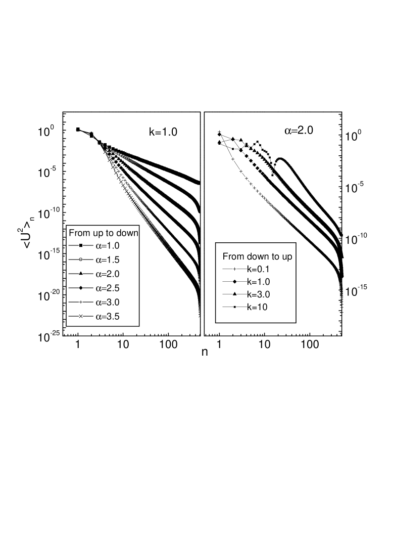
Figure 5: The averaged matrix elements $<U^{2}>$ for different parameters $\alpha$ and $k$. a) right; b) left.

IV Localization length

As shown above, for nonanalytic system, the quantum localization is characterized by the power-law decay of the eigenvector in momentum coordinates. To give a quantitative description of the localization phenomenon in nonanalytic systems, let us investigate the localization length advocated iniz ; casati2 :

$$l=Nexp(<\sl{H}>-\sl{H}_{R}),$$ (10)

Here $H$ denotes the information entropy for a (N+1)-dimensional eigenvector $\Phi_{\lambda}(n)(n=-\frac{N}{2},...\frac{N}{2})$, $\sl{H}\equiv-\sum_{n}\Phi_{\lambda}^{2}(n)ln(\Phi_{\lambda}^{2}(n))$, and the symbol $<...>$ represents an average over all eigenvector; The normalizing coefficient $H_{R}$ determines the maximal value of entropy.

The above definition is one of commonly used in the analytic models such as KR model, it can be extended to nonanalytic systems for the information entropy defined for a eigenvector is convergence for $\alpha>0.5$.

At $\alpha=\infty$, our model is equivalence to the well studied model KR model. In this case, there exist a additional integral, the parity. Together with the time-reversal symmetry, the eigenfunction can be expressed by a real function with the relation $\Phi_{\lambda}(n)=\pm\Phi_{\lambda}(-n)$. So the total number of the independent components of is $N_{1}=N/2$, it satisfies following Gaussian distribution (e.g. refer to iz ),

$$W(|\Phi_{\lambda}(n)|)=2\sqrt{N_{1}/\pi}e^{-\Phi_{\lambda}^{2}(n)N_{1}}.$$ (11)

Then this analysis gives a implicit expression of the maxium entropy as $H_{R}\simeq ln(0.48N)$.

In the case $\alpha\neq\infty$, the parity symmetry is broken, the eigenfunctions have different real and imaginary parts. Both of them satisfy the Gaussian distribution except for $N_{1}=N$, then the module of the components should satisfy following Wigner-type distribution,

$$W(|\Phi_{\lambda}(n)|)=2N_{1}|\Phi_{\lambda}(n)|e^{-\Phi_{\lambda}^{2}(n)N_{1}}.$$ (12)

Our numerical calculations verify the above distribuation (Fig.6) and gives the maximal value of information entropy as $H_{R}\simeq ln(0.7N)$.

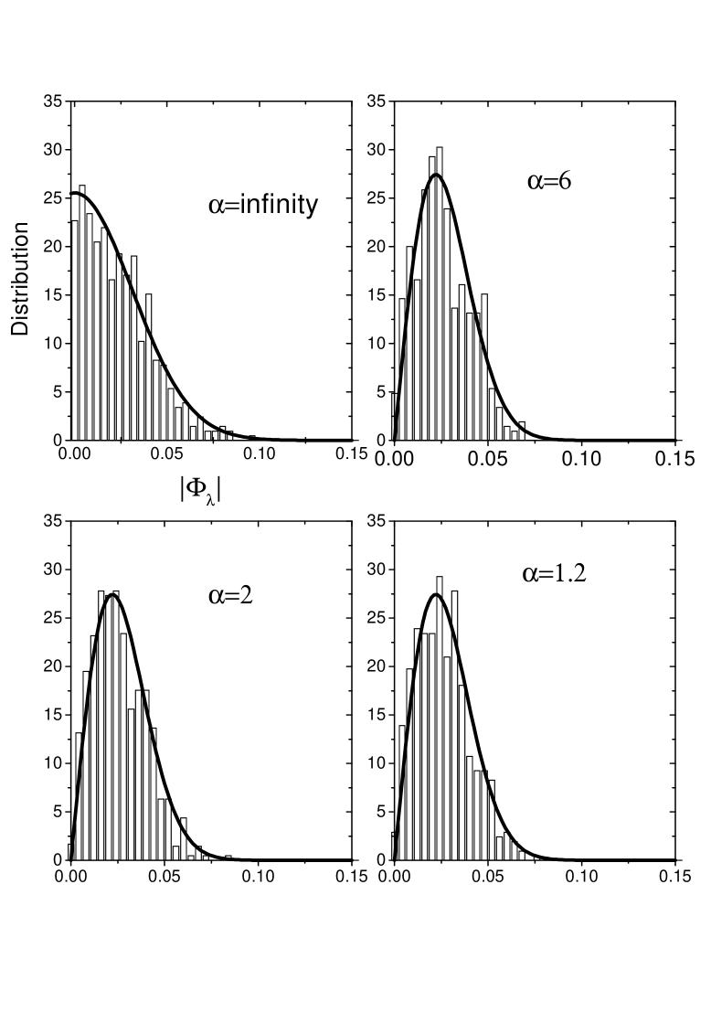
Figure 6: The distribution of the typical completely extended eigenstates for various $\alpha$. The smooth curves are distribution expressed by Eq.(11) and Eq.(12), respectively.

We calculate the dependence of the localization length on the perturbation strength for the different parameter $\alpha$ (Fig.7a). It is shown, the plots of the localization length vs. perturbation amplitude k can be divided into four parts: perturbative localization regime, pseudo-integral regime, dynamical localization regime, and saturation regime. Each regime is characterized by the different relation between the localization length and the perturbation strength.

In the perturbative regime ($k<1$), average entropy shows linearly proportional to $k$, i.e. $ln(l)\sim k$ (Fig.7c). In this regime, the Floquet state in momentum representation can be well fitted by the Lorentz-like distribution.

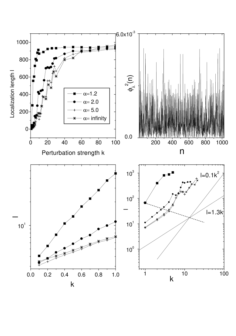
Figure 7: $\frac{a|b}{c|d}$. a) Localization length vs. perturbation strength for different $\alpha$; b) In the saturation regime, a typical completely extended eigenvector for $\alpha=5$ and $k=300$; c) In the perturbative regime, it is clearly shown $ln(l)\sim k$; d) The dashed line corresponds to the critical values $K_{cl}$ for different $\alpha$, approximately. In the downside of the dashed line, i.e. pseudo-integral regime, it is clearly shown $l\sim k$. In the dynamical localization regime (upside of the dashed line), it is clearly shown $l\sim k^{2}$.

If $k$ is large enough, one observe a kind of saturation, i.e. the localization length almost keep constant, no longer increases with the $k$. This implies that eigenstates have become completely delocalized (Fig.7b). The limit value of the length almost tends to $N$, the maximum localization length.

In the intermediate $k$ i.e. $N>l$ and $k>1$, the typical property of the eigenfunctions is the power-law tail. The power exponent tightly relates the convergence rate of the Fourier expansion of the external potential. In this regime, as the perturbation is large enough, i.e. $k>k_{cr}$, the phase space will show ergodicity. In this case, it is clearly shown that the localization length is proportional to the square of the perturbation strength i.e. classical diffusion rate $D_{cl}$ (Fig.7d, upside of the dashed line),

$$l\sim k^{2}.$$ (13)

However, in the case of that perturbation is not so strong, the phase space seems not ergodic. In this case, even though the KAM tori are broken down, the cantori and other invariant structures may act as barriers for the quantum motions, if the flux through cantori is less than one Planck’s cell (for example, see middle column of the Fig.2). The eigenstates are expected to localized on these invariant structures. Indeed, in such situation the quantum system looks as if classical integrable, i.e. so called pseudo-intergrable regime bbb1 ; bbb2 ; bbb3 . In this case, the eigenstates still can be approximately fitted by the Lorentz-like distribution (Fig.8). Furthermore, we find that in this regime the localization length show linearly proportional to the perturbation strength (Fig.7d, downside of the dashed line),

$$l\sim k.$$ (14)

This regime become more and more narrow as we decrease the $\alpha$. As $\alpha<1.5$, the classical coefficient tends to infinite which means that flow rather than diffusion occurs. In this case, the localization length transits directly from perturbative regime to the square scaling-law regime (see Fig.7d, case $\alpha=1.2$).

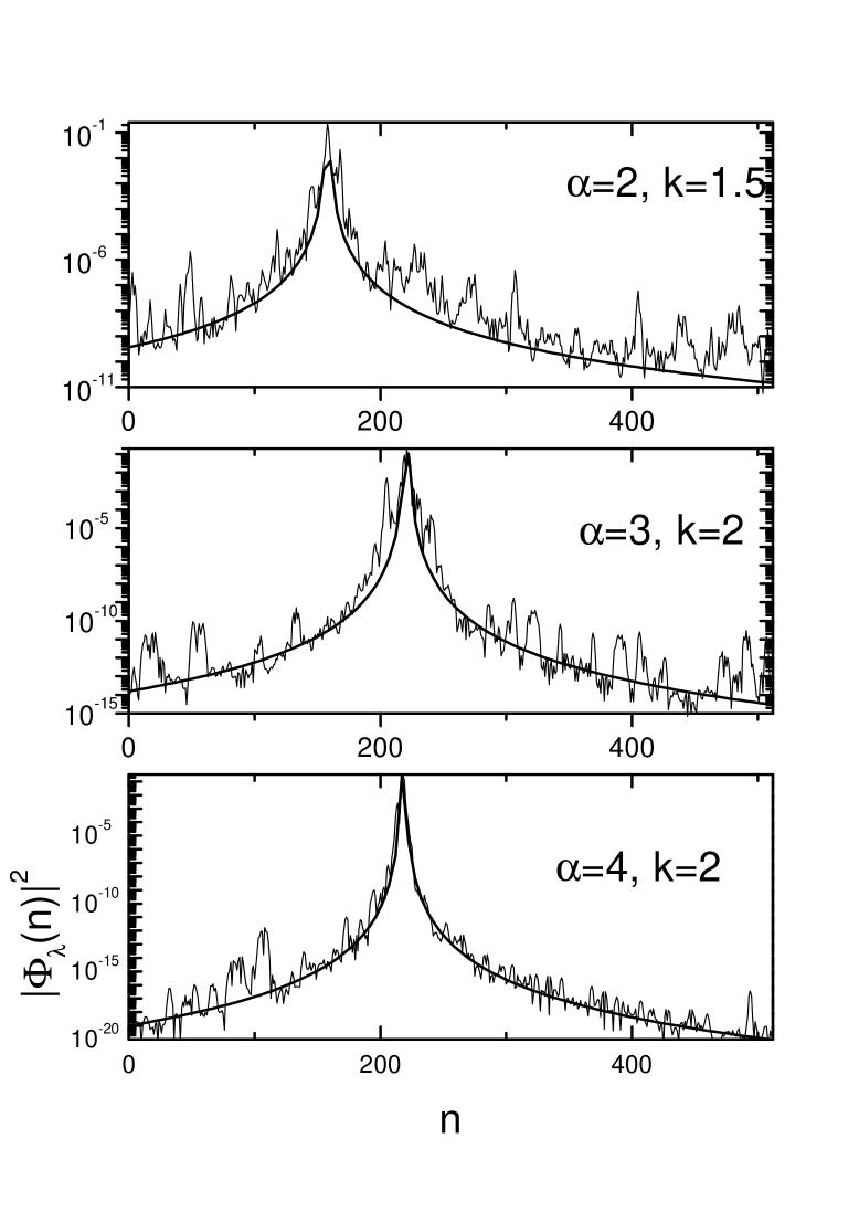
Figure 8: Typical eigenstates in the pseudo-integral regime. The smooth curves represent the Lorentz-like distributions (Eq.8).

V Energy Diffusion

The energy diffusion of KR model has been well studied. After a typical time scale, the energy diffusion will be completely suppressed. For this model, Floquet states show the strong localization (exponential decay) in momentum representation, which implies that, only a finite number of Floquet states can be excited for any initial state. The question is that what happens to the energy diffusion in the nonanalytic models, where the Floquet states are not so ’strong’ localized, only the power-law type localization is observed from the above sections. In the dynamical localization regime, out of a chaotic band, the tails of the Floquet states behave as $|\Phi_{\lambda}(n)|^{2}\sim\frac{1}{n^{2\alpha}}$, so the average energy approximates to $\sum_{n}\frac{1}{n^{2\alpha}}\times 2n^{2}$, which is divergence for $\alpha\leq 1.5$. From this analysis, we conjecture that the diffusion suppression will be relaxed as we decrease the parameter $\alpha$, i.e. lowering the derivable degree of the system.

We make a numerical simulation to test the above deduction. To ensure the precision of the numerical simulation, both coordinate and momentum spaces should be large enough, so a large number (N=32768) of Fourier components are used in our computations. We rescale the coefficients $C_{\alpha}$ so that the classical diffusion rate $D_{cl}\simeq D_{ql}=k^{2}/2$ in the quasilinear approximation. To satisfy the condition, $C_{\alpha}=0.129,0.219,0.759,$ and $1.00$ at $\alpha=1.52,1.60,2.00$ and $\infty$, respectively. Our results are shown in Fig.9. The complete suppression of the diffusion is relaxed, instead, a kind of quantum diffusion is clearly evident as $\alpha$ be $1.52$ and $1.60$. Our system is isolated from the environment, the observed delocalization is completely due to the nonanalyticity of the the system, which leads to the possibility of a long-range hopping in the momentum space. On the other aspect, we find that, as $\alpha\geq 2$, the diffusion is completely suppressed.

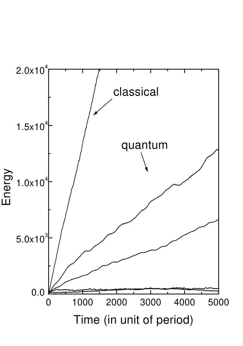
Figure 9: The energy diffusion for different parameters $\alpha$ at $k=6$. Classically, the 1000 initial points are distributed in $p=0$ with the random $q$ and evolved by the map Eq.(4) at $\alpha=\infty$. For other $\alpha$, since the $C_{\alpha}$ is recaled, in the quasilinear approximation, the classical evolution shows the similar behavior. Quantumly, the initial state is chosen as the ground state $|0\rangle$ of unperturbed system. The curves from the up to down correspond to $\alpha=1.52,1.60,2.00$ and $\infty$. It is clearly shown that as $\alpha\geq 2$ the diffusion is completely suppressed. Otherwise, a kind of quantum diffusion occurs.

VI Conculsions

In summary, nonanalytic systems show many interesting properties, the parameter $\alpha$ which represents the convergence rate of the Fourier series determines the type of the evolution matrix, therefore plays an important role. Even though our discussion is towards a special choice of the potential, the conclusions are generic. The Fourier coefficients of any nonanalytic potential take form of $c_{n}/n^{\alpha}$. Previously known nonanalytic models are Fermi-acceleration modelfcm , billiad system bs1 ; bs2 and a kicked particle in 1D infinite square potential wellblgh . Their common feature is the algebraic decay of the evolution matrix elements, the corresponding parameter $\alpha$ equals to one, two and two, respectively. In the general nonanalytic case, our studies reveal four different regimes: perturbative, pseudo-integral, dynamical localization and complete extension. In each regime, the relation between the localization length and the perturbation strength is found to follow different scaling law. This finding is in agreement with the arguments in previous works bbb1 ; bbb2 ; bbb3

On the other hand, it was found that declocalization occurs if one let the system interact with an environment. This became an active point attracting much attention theoretical and experimentally in recent years. Our findings in this paper suggest that declocalization can be realized by breaking the analyticity of the system. We hope our works will stimulate the studies in the direction.

References

- (1) G.Casati, B.V.Chirikov, J.Ford, and F.M.Izrailev, Lect. Notes Phys. 93, 334 (1979).
- (2) B.V.Chirikov, Phys. Rep. 52, 263 (1979); F.M.Izrailev, Phys.Rep. 196, 299 (1990); G.Casati and B.V.Chirikov, Quantum Chaos (Cambridge University Press, Cambridge, 1995).
- (3) For example to see, A.K.Dhar, M.A.Nagaranjan, F.M.Izrailev, and R.R.Whitehead, J.Phys.B 16, L17 (1983); C.F.Hillermeier, R.Blumel, and U.Smilansky, Phys.Rev. A 45, 3486 (1992); G.Casati, I.Guarneri, and G.Mantica, Phys.Rev.A 50, 5018 (1994); C.O.Reinhold, J.Burgdorfer, M.T.Frey and F.B.Dunning, Phys.Rev.Lett. 79, 5226 (1997)
- (4) E.J.Galvez, B.E.Sauer, L.Moorman, P.M.Kock, and D.Richards, Phys.Rev.Lett. 61, 2011 (1988); J.E.Bayfield, G.Casati, I.Guarneri, and D.Sokol, ibid 63, 364 (1989); M.Arndt, A.Buchleitner, R.N.Mantehna, and H.Walther ibid 67, 2435 (1991)
- (5) Jorge V.Jose and Robert Cordery, Phys.Rev.Lett. 56, 290, (1986)
- (6) F.Borgonovi, G.Casati, and B.Li, Phys.Rev.Lett. 77 4744 (1996)
- (7) F.Borgonovi, Phys.Rev.Lett. 80, 4653 (1998)
- (8) B.Hu,B.Li, J.Liu, and Y.Gu, Phys.Rev.Lett. 82, 4224 (1999)
- (9) G.Casati, T.Prosen, ’The quantum mechanics of chaotic biliards’, cond-mat/9803360, to appear in Physica D (1999)
- (10) F.Borgonovi, P.Conti, D.Rebuzzi, B.Hu, and B.Li, ’Cantori and dynamical localization in the Bunimovich Stadium’, cond-mat/9807300, to appear in Physica D (1999)
- (11) G.Casati, T.Prosen, Phys. Rev. E, 59, R2516 (1999)
- (12) M.R.Herman, Sur les courbes invariantes par les diffemorphisma de lanneau, Asterisque, 103-104 (1983)
- (13) B. Hu, B. Li, J. Liu and J. L. Zhou, Phys. Rev. E 58 No. 2, 1743 (1998).
- (14) A.M.Mirlin, Y.V.Fyodorov, F.M.Dittes, J.Quezada and T.H.Seligman, Phys.Rev.E 54, 3221 (1996).
- (15) F.M.Izrailev, J.Phys.A: Math.Gen. 22, 865 (1989)
Figures Captions
Fig.1 The nonanalytic potential functions .
Fig.2 Local phase plane for various parameters. As and , the phase plane is ploted by tracing one trajectory originated from the stochastic region for ten thousands or more periods.
Fig.3 Classical diffusion coefficients versus the perturbation strength for various .
Fig.4 The typical eigenvectors in momentum representation for different parameters. The smooth curves represent the Lorentz-like distributions (Eq.8). The relation between power exponent and the parameter is .
Fig.5 The averaged matrix elements for different parameters and . a) right; b) left.
Fig.6 The distribution of the typical completely extended eigenstates for various . The smooth curves are distribution expressed by Eq.(11) and Eq.(12), respectively. Fig.7 . a) Localization length vs. perturbation strength for different ; b) In the saturation regime, a typical completely extended eigenvector for and ; c) In the perturbative regime, it is clearly shown ; d) The dashed line corresponds to the critical values for different , approximately. In the downside of the dashed line, i.e. pseudo-integral regime, it is clearly shown . In the dynamical localization regime (upside of the dashed line), it is clearly shown .
Fig.8 Typical eigenstates in the pseudo-integral regime. The smooth curves represent the Lorentz-like distributions (Eq.8).
Fig.9 The energy diffusion for different parameters at . Classically, the 1000 initial points are distributed in with the random and evolved by the map Eq.(4) at . For other , since the is recaled, in the quasilinear approximation, the classical evolution shows the similar behavior. Quantumly, the initial state is chosen as the ground state of unperturbed system. The curves from the up to down correspond to and . It is clearly shown that as the diffusion is completely suppressed. Otherwise, a kind of quantum diffusion occurs.