Active and passive fields face to face

Abstract

The statistical properties of active and passive scalar fields transported by the same turbulent flow are investigated. Four examples of active scalar have been considered: temperature in thermal convection, magnetic potential in two-dimensional magnetohydrodynamics, vorticity in two-dimensional Ekman turbulence and potential temperature in surface flows. In the cases of temperature and vorticity, it is found that the active scalar behavior is akin to that of its co-evolving passive counterpart. The two other cases indicate that this similarity is in fact not generic and differences between passive and active fields can be striking: in two-dimensional magnetohydrodynamics the magnetic potential performs an inverse cascade while the passive scalar cascades toward the small-scales; in surface flows, albeit both perform a direct cascade, the potential temperature and the passive scalar have different scaling laws already at the level of low-order statistical objects. These dramatic differences are rooted in the correlations between the active scalar input and the particle trajectories. The role of such correlations in the issue of universality in active scalar transport and the behavior of dissipative anomalies is addressed.

1 Introduction

Scalar fields transported by turbulent flows are encountered in many natural phenomena and engineering problems, ranging from atmospheric physics [1] to combustion [2], to the transport and amplification of magnetic fields in astrophysical fluids [3]. Here, we consider the case of advected scalar fields such as temperature, pollutant density, chemical or biological species concentration.

In many cases there is a two-way coupling between the scalar and the flow: the transported field can influence the velocity field – this is dubbed active transport. This is the case, for example, of the temperature field that acts on velocity through buoyancy forces. Conversely, situations where the feedback of the scalar field is negligible and the velocity determines the properties of the scalar, but not vice versa are known as passive. This ideal case is well approximated by fluorescent dye used in laboratory experiments to mark fluid parcels.

Although active and passive scalars are governed by the same advection-diffusion equation, their nature is radically different. Passive scalars belong to the realm of linear problems, even though highly nontrivial. Indeed, as a consequence of the statistical independence of the forcing and the advecting velocity, the transported field depends linearly on the forcing. This property allows a full-fledged theoretical treatment of the problem, and has the major consequence that the passive scalar scaling laws are universal with respect to the injection mechanism. On the contrary, for active fields the presence of the feedback couples the velocity to the transported scalar and makes the problem fully nonlinear. In this case, the theoretical tools developed for the study of the passive problem may fall short of explaining the behavior of active scalars, and, as of today, the understanding of active turbulent transport lags far behind the knowledge accumulated for the passive counterpart. This state of the art motivated us to pursue a “case study” of turbulent transport of active and passive scalars, using the scaling properties of fields evolving in the same turbulent flow as the basic diagnostics for comparison.

We consider four different systems belonging to the two following general classes of problems: (i) active scalars that influence the flow through local forces; (ii) active fields functionally related to the velocity.

The evolution of a scalar belonging to the first class is described in terms of the following set of equations:

$$\partial_{t}a+{\bm{v}}\cdot{\bm{\nabla}}a = \kappa\Delta\,a+f_{a}\;,$$ (1)

$$\partial_{t}c+{\bm{v}}\cdot{\bm{\nabla}}c = \kappa\Delta\,c+f_{c}\;,$$ (2)

$$\partial_{t}{\bm{v}}+{\bm{v}}\cdot{\bm{\nabla}}{\bm{v}} = -{\bm{\nabla}}p+\nu\Delta{\bm{v}}+{\bm{F}}[a,{\bm{\nabla}}a,\dots]\;,$$ (3)

where $a$ and $c$ are the active and passive scalar fields, respectively and obey the advection-diffusion equations (1) and (2). The scalar inputs $f_{a}$ and $f_{c}$ have a characteristic lengthscale $\ell_{f}$, and represent two different realizations of the same stochastic process. Were they coincident, no difference between active and passive fields would persist. For the sake of simplicity, we use the same molecular diffusivity, $\kappa$ for both scalars. The active character of $a$ is embodied by the term ${\bm{F}}[a,{\bm{\nabla}}a,\dots]$, which acts as a forcing for the velocity field in the Navier-Stokes equations. The specific form of the ${\bm{F}}$ term depends on the physical system under investigation. In the following we shall consider two examples from this class: thermal convection [4, 5], where $a$ is the temperature field and ${\bm{F}}=-\beta a{\bm{g}}$ is the buoyancy force, and two-dimensional magnetohydrodynamics [6], where $a$ is the magnetic potential and ${\bm{F}}=-\Delta a{\bm{\nabla}}a$ is the Lorentz force.

The second class of active scalars is relevant to geophysical flows [7, 8]. In this case the dynamics is described in terms of a scalar field obeying the advection-diffusion equation (1), supplemented by a functional relation that gives ${\bm{v}}$ in terms of $a$ :

$$v_{i}({\bm{x}},t)=\int\Gamma_{i}({\bm{x}}-{\bm{y}})a({\bm{y}},t){\rm d}{\bm{y}}\,.$$ (4)

Here, the vector valued kernel ${\bm{\Gamma}}$ is divergence-free. A well-known instance from such class is the two-dimensional Navier-Stokes equation, where the active scalar is the vorticity, ${\bm{\nabla}}\times{\bm{v}}$. Another problem which we shall discuss is the turbulent flow on the flat surface of an infinitely high fluid, described by the surface-quasi-geostrophic equation [9, 10]. Here, the active scalar is the fluid density, which is related (e.g. for ideal gases) to the so-called potential temperature.

Some of the results presented in this paper were previously discussed in Refs. [11, 12, 13]. Related investigations on active and passive transport may be found in [14, 15] and [16, 17].

The paper is organized as follows. In Sect. 2, we briefly review some results about passive scalar transport in turbulent flows. Particular emphasis is put on the Lagrangian description of scalar transport, pointing out the results which hold for active scalars as well. In Sect. 3 the statistics of the (active) temperature and a passive scalar field in $2d$ convection is discussed. Sect. 4 is devoted to the analysis of two-dimensional magnetohydrodynamics, with a thorough discussion of the problem of dissipative anomaly in scalar transport. In Sect. 5 the evolution of passive and active fields in Ekman-Navier-Stokes turbulence is discussed. In Sect. 6 we study the properties of turbulence on fluid surfaces under the quasi-geostrophic approximation. In the last section we summarize the main findings and delineate the perspectives for active scalar transport.

2 Passive scalar turbulence

2.1 Eulerian approach

The dynamics of passive scalars is governed by the advection diffusion equation (2). In order to describe the general properties of passive scalar evolution in turbulent incompressible velocity fields, we assume that the velocity field ${\bm{v}}$ is scale invariant and rough. In other words, the spatial increments $\delta_{r}v\!=\!({\bm{v}}({\bm{x}}\!+\!{\bm{r}},t)\!-\!{\bm{v}}({\bm{x}},t))\cdot{\bm{r}}/r$ depend on the separation $r$ as a fractional power, i.e. $\delta_{r}v\sim r^{h}$ with $h<1$ (e.g. $h=1/3$ in Kolmogorov’s 1941 turbulence [18]). Being interested in the statistically steady properties of the field, we introduce a source of scalar fluctuations $f_{c}$. In the following we take for convenience a random, Gaussian, statistically homogeneous and isotropic forcing with zero mean and correlation function

$$\langle f_{c}({\bm{x}}_{1},t)f_{c}({\bm{x}}_{2},t^{\prime})\rangle=\delta(t-t^{\prime}){\cal F}(|{\bm{x}}_{1}-{\bm{x}}_{2}|/\ell_{f})\,.$$ (5)

The correlation function of the forcing ${\cal F}(r/\ell_{f})$ is roughly constant at scales smaller than $\ell_{f}$, which is assumed to be within the scaling range of ${\bm{v}}$, and drops rapidly to zero for $r>\ell_{f}$.

The phenomenology of passive scalar turbulence may be summarized as follows. Scalar fluctuations injected at the scale $\ell_{f}$ are transferred toward the small scales with a constant flux, down to the dissipative scale $\ell_{d}$. There, the molecular diffusion absorbs the incoming flux and ensures the equilibrium between the input and the dissipation. The fluctuations are thus maintained in a statistically steady state which is characterized by two major properties. First, the scalar dissipation is asymptotically independent of the molecular diffusivity $\kappa$, attaining a finite nonzero limiting value for $\kappa\to 0$. This singular behavior of the dissipation is also known as dissipative anomaly. Second, in the scaling range $\ell_{d}\ll r\ll\ell_{f}$ the scalar statistics is intermittent. This amounts to saying that the small-scale statistics is characterized by the alternance of strong, rare events where the scalar increments, $\delta_{r}c\!=\!c({\bm{x}}\!+\!{\bm{r}},t)\!-\!c({\bm{x}},t)$ are much larger than their typical value, $c_{rms}\,$, and long quiescent phases where $\delta_{r}c\ll c_{rms}$. Intermittency is reflected by the scaling behavior of the structure functions, i.e. the moments of the scalar increments

$$S^{c}_{N}(r)=\langle(\delta_{r}c)^{N}\rangle\propto r^{\zeta^{dim}_{N}}\left({\ell_{f}\over r}\right)^{\zeta^{dim}_{N}-\zeta^{c}_{N}}\,.$$ (6)

The scaling exponents $\zeta^{c}_{N}$ are said to be anomalous, when they deviate from the dimensional expectation $\zeta^{dim}_{N}=N(1-h)/2$. The equality $\zeta^{c}_{N}=\zeta^{dim}_{N}$ holds possibly only for $N=2$ [4], whereas for $N>2$ the deviations become more and more severe. The asymptotic behavior at large orders $N$ corresponds to the saturation $\zeta^{c}_{N}\to\zeta^{c}_{\infty}$ [21]. The saturation is related to the presence of sharp “fronts” in the scalar field. The exponents $\zeta^{c}_{N}$ are universal with respect to the details of the energy injection statistics. The forcing only affects the numerical prefactors appearing in the structure functions.

The anomalous scaling $\zeta^{dim}_{N}\neq\!\zeta^{c}_{N}$ signals the breakdown of scale invariance, as confirmed by the explicit appearance of $\ell_{f}$ in (6), even at scales $r\!\ll\!\ell_{f}$. Indeed, anomalous scaling of the moments of scalar increments is equivalent to state that the probability density functions (pdf’s) of $\delta_{r}c$ at different $r$’s cannot be collapsed by rescaling them with a unique power law in $r$. Even though the specific values of the exponents $\zeta^{c}_{N}$ depend on the details of the flow (statistics, time correlation, and roughness exponent $h$), intermittency and the breaking of scale invariance in the scalar statistics are generic features of passive scalar turbulence.

The physical mechanism leading to anomalous scaling has been recently understood in the framework of the Kraichnan model of scalar advection [22, 23] (see Refs. [24, 25, 26] and Ref. [27] for an exhaustive review on the subject). In this model the advecting flow ${\bm{v}}$ is random, Gaussian, self-similar and $\delta$-correlated in time. Under these special conditions, there exists a closed set of linear equations for multi-point correlation functions. The anomalous exponents are the scaling exponents of the homogeneous solutions (the so-called zero modes) of those equations. Since homogeneous solutions do not depend by definition on the scalar input, their scaling exponents are universal, and cannot be inferred from dimensional arguments. The concept of zero mode can be extended to passive scalar turbulence in generic velocity fields [28].

The properties of passive scalars described up to now are in the language of fields –the Eulerian description. It is now interesting to adopt a different but equivalent viewpoint in terms of particle trajectories –the Lagrangian description.

2.2 Lagrangian description

The basic idea of the Lagrangian approach is to solve Eq. (2) by the method of characteristics. Let us denote ${\bm{\rho}}(s;{\bm{x}},t)$ (henceforth whenever there is no ambiguity we indicate it as ${\bm{\rho}}(s)$) as the trajectory of a fluid particle landing at point ${\bm{x}}$ at time $t$. The path ${\bm{\rho}}(s)$ is the solution of the stochastic differential equation

$${d{\bm{\rho}}(s)\over ds}={\bm{v}}({\bm{\rho}}(s),s)+\sqrt{2\kappa}\,\dot{\bm{w}}(s)\,,\qquad{\bm{\rho}}(t)={\bm{x}}\,,$$ (7)

where $i,j=1,\dots,d$ ($d$ being the space dimensionality), and $\dot{\bm{w}}(s)$ is a Wiener process (the derivative of a Brownian motion), i.e. $\dot{w}_{i}$ are Gaussian variables of zero mean and correlation $\langle\dot{w}_{i}(s)\dot{w}_{j}(s^{\prime})\rangle=\delta_{ij}\delta(s-s^{\prime})$. Along the path ${\bm{\rho}}(s)$ Eq. (2) reduces to

$${d\phi^{\bm{w}}(s)\over ds}=f_{c}({\bm{\rho}}(s),s)\,,$$ (8)

which is easily solved as $\phi^{\bm{w}}(t)=\int_{0}^{t}{\rm d}s\,f_{c}({\bm{\rho}}(s),s)$. For the sake of simplicity, we assumed $\phi^{\bm{w}}(0)=0$. We indicated with $\phi^{\bm{w}}$ the solution obtained along the path ${\bm{\rho}}$ obtained for a specific realization of the process ${\bm{w}}$. The passive scalar field, $c({\bm{x}},t)$, is recovered by averaging over all the realizations of ${\bm{w}}$, i.e. along all the Lagrangian paths ending in ${\bm{x}}$ at time $t$ [29]:

$$c({\bm{x}},t)=\langle\phi^{\bm{w}}(t)\rangle_{\bm{w}}=\left\langle\int_{0}^{t}{\rm d}s\,f_{c}({\bm{\rho}}(s),s)\right\rangle_{\bm{w}}\,.$$ (9)

The statistic of the trajectories is summarized in the particle propagator $P({\bm{y}},s|{\bm{x}},t)=\langle\delta({\bm{y}}-{\bm{\rho}}(s;{\bm{x}},t)\rangle_{\bm{w}}$, that is the probability of finding a particle at point ${\bm{y}}$ and time $s\leq t$, provided it is in ${\bm{x}}$ at time $t$. According to the theory of stochastic processes [30], $P({\bm{y}},s|{\bm{x}},t)$ obeys the Kolmogorov equations:

$$-\partial_{s}P({\bm{y}},s|{\bm{x}},t)-{\bm{\nabla}}_{\!y}\cdot[{\bm{v}}({\bm{y}},s)P({\bm{y}},s|{\bm{x}},t)]\! = \!\kappa\Delta_{y}P({\bm{y}},s|{\bm{x}},t)\,,$$ (10)

$$\;\;\;\partial_{t}P({\bm{y}},s|{\bm{x}},t)+{\bm{\nabla}}_{\!x}\cdot[{\bm{v}}({\bm{x}},t)P({\bm{y}},s|{\bm{x}},t)]\! = \!\kappa\Delta_{x}P({\bm{y}},s|{\bm{x}},t)\,,$$ (11)

with initial condition $P({\bm{y}},t|{\bm{x}},t)=\delta({\bm{x}}-{\bm{y}})$. The unusual minus signs in the l.h.s. of (10) are due to the fact that particles move backward in time. The solution of (2) can be written in terms of the propagator:

$$c({\bm{x}},t)=\int_{0}^{t}ds\int d{\bm{y}}\,f_{c}({\bm{y}},s)P({\bm{y}},s|{\bm{x}},t)\;,$$ (12)

as it can be directly checked by inserting (12) in (2) and using (11).

At variance with smooth velocities (i.e. Lipschitz continuous, $\delta_{r}v\sim r$) where for $\kappa\to 0$ particle trajectories are unique, for velocity fields rough and incompressible the particle propagator does not collapse onto a single trajectory in the limit $\kappa\to 0$. Lagrangian paths are not unique and initially coincident particles separate in a finite time. This property is at the root of the dissipative anomaly.

For active and passive scalars evolving in the same flow, the Lagrangian paths ${\bm{\rho}}(s)$ are the same, as well as the propagator $P({\bm{y}},s|{\bm{x}},t)$. The difference between $a$ and $c$ is that, since the active scalar enters the dynamics of ${\bm{v}}$ (3-4), the Lagrangian trajectories are functionally related to the active scalar forcing $f_{a}$, but are independent of the passive source term $f_{c}$. This is the Lagrangian counterpart of the linearity of the passive scalar problem, which does not hold for the more complicated case of active scalars.

One of the advantages of the Lagrangian description is that it makes transparent the physics of transport processes. For instance, let us consider the $2$-points correlation function for passive scalars, ${\cal C}^{c}({\bm{x}}_{1},{\bm{x}}_{2};t)=\langle c({\bm{x}}_{1},t)c({\bm{x}}_{2},t)\rangle$. This offers the possibility of an intuitive interpretation of the energy cascade phenomenology and gives insights into measurable statistical objects such as the scalar spectrum $E_{c}(k)$, that is the Fourier transform of ${\cal C}^{c}_{2}$. From (9) and averaging over $f_{c}$ and ${\bm{v}}$ one obtains

$${\cal C}^{c}_{2}({\bm{x}}_{1},{\bm{x}_{2}};t)=\left\langle\int_{0}^{t}\!{\rm d}s_{1}\int_{0}^{t}\!{\rm d}s_{2}\left\langle f_{c}({\bm{\rho}}(s_{1};{\bm{x}}_{1},t))f_{c}({\bm{\rho}}(s_{2};{\bm{x}}_{2},t))\right\rangle_{f}\right\rangle_{{\bm{w}}{\bm{v}}}\,.$$ (13)

Introducing the velocity-averaged two-particle propagator $\langle P_{2}({\bm{y}}_{1},{\bm{y}}_{2},s|{\bm{x}}_{1},{\bm{x}}_{2},t)\rangle_{v}$, which evolves according to the straightforward generalization of (10, 11) to two particles, and using (5), Eq. (13) reduces to

$$\qquad{\cal C}^{c}_{2}({\bm{x}}_{1},{\bm{x}_{2}};t)=\int_{0}^{t}{\rm d}s\int\int\langle P_{2}({\bm{y}}_{1},{\bm{y}}_{2},s|{\bm{x}}_{1},{\bm{x}}_{2},t)\rangle_{v}{\cal F}\left({|{\bm{y}}_{1}-{\bm{y}}_{2}|/\ell_{f}}\right){\rm d}{\bm{y}}_{1}{\rm d}{\bm{y}}_{2}\,,$$ (14)

which has a clear physical interpretation. Since ${\cal F}(x)$ is vanishingly small for $x\gg 1$, the correlation ${\cal C}^{c}_{2}$ is essentially the average time spent by a particle pair with a separation $r=|{\bm{x}}_{1}-{\bm{x}}_{2}|$ below the forcing scale $\ell_{f}$. Due to the explosive separation of particles, this time has a finite limit for $r\to 0$, which yields the leading contribution to ${\cal C}^{c}_{2}$. The subleading behavior is uncovered by the second-order structure function

$$S^{c}_{2}(r)=\langle(c({\bm{x}}_{1},t)-c({\bm{x}}_{2},t))^{2}\rangle=2({\cal C}^{c}_{2}(0)-{\cal C}^{c}_{2}(r))\,,$$ (15)

which is roughly the average time ${\cal T}_{\ell_{f}}(r)$ taken by two coinciding particles to reach a separation $r$. For a Kolmogorov 1941 turbulent flow ($h=1/3$) one has $S^{c}_{2}(r)\sim r^{2/3}$, i.e. $E_{c}(k)\sim k^{-5/3}$ – the Oboukov-Corrsin dimensional expectation [4].

The Lagrangian description can be extended also to higher-order statistics as multipoint correlation functions ${\cal C}^{c}_{N}({\bm{x}}_{1},\ldots,{\bm{x}}_{N})=\langle c({\bm{x}}_{1},t)\ldots c({\bm{x}}_{N},t)\rangle$. However, when many points come into play, their geometrical arrangement becomes crucial. Dimensional arguments, which are based on the size of the configuration but forcibly neglect the “angular” information, fall short of capturing the observed behavior for multi-point observables. A detailed discussion of their properties is beyond the scope of this brief review. In the following we just summarize the main concepts, referring to Refs. [31, 27] for further reading.

Expanding the power in the definition of the structure functions $S^{c}_{N}(r)$, it is immediate to express them as a linear combinations of $N$-point correlation functions (see, e.g., (15) for $S^{c}_{2}(r)$). Therefore, the latter must contain a contribution, denoted as ${\cal Z}^{c}_{N}({\bm{x}}_{1},\ldots,{\bm{x}}_{N})$, that carries the anomalous scale dependence: ${\cal Z}^{c}_{N}(\lambda{\bm{x}}_{1},\ldots,\lambda{\bm{x}}_{N})=\lambda^{\zeta^{c}_{N}}{\cal Z}^{c}_{N}({\bm{x}}_{1},\ldots,{\bm{x}}_{N})$ [24, 25, 26]. From a Lagrangian viewpoint, the function ${\cal Z}^{c}_{N}$ has a special property that distinguishes it from a generic scaling function. The remarkable result is that [31, 28]

$$\frac{d}{dt}\langle{\cal Z}^{c}_{N}\rangle_{\cal L}=0\,,$$ (16)

where the derivative $\frac{d}{dt}$ is performed along the trajectories of $N$ particles advected by the flow, and the average is over the ensemble of all trajectories. In other terms, ${\cal Z}^{c}_{N}$ is statistically preserved by the flow [28, 32]. Universality of scaling exponents is then just a byproduct of the definition of statistically preserved structures: since $f_{c}$ does not appear in Eq. (16), the properties of zero modes are insensitive to the choice of the forcing.

2.3 Dissipative anomaly

In spite of the continuous injection of scalar through the pumping $f_{c}$, the second-order moment $\langle c^{2}({\bm{x}},t)\rangle$ does not grow indefinitely even in the limit $\kappa\to 0$. This is due to the existence of a finite nonzero limit of the scalar dissipation $\epsilon_{c}=\kappa|{\bm{\nabla}c}|^{2}$ – the dissipative anomaly.

In order to understand how $\langle c^{2}({\bm{x}},t)\rangle$ achieves a finite value independent of the diffusivity coefficient, we adopt the Lagrangian viewpoint. From Eq. (13) we have:

$$\langle c^{2}({\bm{x}},t)\rangle\!\!=\!\!\left\langle\int_{0}^{t}\int_{0}^{t}{\rm d}s_{1}{\rm d}s_{2}f_{c}({\bm{\rho}}(s_{1};{\bm{x}},t))f_{c}({\bm{\rho}}(s_{2};{\bm{x}},t))\right\rangle=\left\langle\left(\int_{0}^{t}{\rm d}sf_{c}({\bm{\rho}}(s;{\bm{x}},t))\right)^{2}\right\rangle\,,$$ (17)

where the brackets indicate the average over the scalar forcing, the velocity field and the noise.

Looking naïvely at (17) one might expect that for a large class of random forcing of zero mean the r.h.s of the above expression would grow linearly with $t$. For instance, when the forcing is Gaussian and $\delta$-correlated in time, one could argue that (17) is essentially a sum of independent variables and by central limit theorem arguments conclude that $\langle c^{2}\rangle\propto t$. This conclusion would be correct if in the limit $\kappa\to 0$ all trajectories collapse onto a unique Lagrangian path. This turns out to be the case for strongly compressible flows but not in general. For compressible flows, energy indeed grows linearly in time and the advected scalar performs an inverse cascade process [33, 34]. On the contrary, in rough incompressible flows coinciding particles typically separate in a finite time, giving rise to multiple paths. As a consequence, a self-averaging process takes place in (17) and this prevents the indefinite growth of the energy. This is evident upon rewriting (17) as

$$\langle c^{2}({\bm{x}},t)\rangle=\int_{0}^{t}{\rm d}s\int\int\langle P_{2}({\bm{y}}_{1},{\bm{y}}_{2},s|{\bm{x}},{\bm{x}},t)\rangle_{v}{\cal F}\left({|{\bm{y}}_{1}-{\bm{y}}_{2}|/\ell_{f}}\right){\rm d}{\bm{y}}_{1}{\rm d}{\bm{y}}_{2}\,.$$ (18)

The time integral is cut off at $|t-s|\gg{\cal T}_{\ell_{f}}$, that is for times larger than the (finite) time needed by two coinciding particles to separate by a distance larger than the forcing correlation length $\ell_{f}$. This is the mechanism leading to a finite dissipation of energy. To summarize, the incompressibility and the roughness of the flow result in the dissipative anomaly through the explosive separation of particle paths. Further discussion on the role of dissipative anomaly in passive scalar turbulence can be found in [23, 33, 35].

3 Two-dimensional turbulent convection

An interesting problem in the context of turbulent transport is the advection of inhomogeneous temperature fields in a gravitational field. Temperature fluctuations induce density fluctuations that in turn, via buoyancy forces, affect the velocity field: hence the temperature field is an active scalar [4, 5]. Here, we consider two-dimensional convection, which is also of experimental interest in Hele-Shaw flows [36]. As an additional asset, the two-dimensional problem is better suited for the study of scaling properties since it allows to reach higher resolution and larger statistics.

Two-dimensional convection is described by the following equations

$$\partial_{t}a+{\bm{v}}\cdot{\bm{\nabla}}a = \kappa\Delta\,a+f_{a}\;,$$ (19)

$$\partial_{t}{\bm{v}}+{\bm{v}}\cdot{\bm{\nabla}}{\bm{v}} = -{\bm{\nabla}}p+\nu\Delta{\bm{v}}-\beta a{\bm{g}}-\alpha{\bm{v}}\,,$$ (20)

where $a$ is the field of temperature fluctuations. The second equation is the two-dimensional Navier-Stokes equation where ${\bm{v}}$ is forced by the buoyancy term $-\beta{\bm{g}}a$ in the Boussinesq approximation [4]; ${\bm{g}}=g\hat{\bm{y}}$ is the gravitational acceleration and $\beta$ the thermal expansion coefficient. Kinetic energy is removed at the large scales by the friction term, $-\alpha{\bm{v}}$. The friction is physically due to the drag experienced by a thin (quasi $2d$) layer of fluid with the walls or air [7, 37]; $\alpha$ is related to the thickness of the fluid layer. A passive scalar, $c$, evolving according to Eq. (2) in the same flow has been considered as well, for comparison.

Before entering in the active/passive scalar issue, let us briefly recall the phenomenology of 2D turbulent convection (for the 3D case see, e.g., [4, 5]). The balance of buoyancy and inertial terms in (20) introduces the Bolgiano lengthscale $\ell_{B}$. [4]. At small scales, $r\ll\ell_{B}$, the inertial term is larger than buoyancy forces and the temperature is basically a passive scalar. At large scales, $r\gg\ell_{B}$, buoyancy dominates and affects the velocity, which in two dimensions performs an inverse energy cascade. However, at variance with the usual 2D Navier-Stokes turbulence, the kinetic energy input rate $\varepsilon$ depends here on the scale. Dimensional arguments yield $\varepsilon(r)=\beta{\bm{g}}\cdot\langle{\bm{v}}({\bm{x}}+{\bm{r}},t)a({\bm{x}},t)\rangle\sim r^{4/5}$, the Bolgiano scaling for the velocity structure functions

$$S^{v}_{N}(r)\sim(\varepsilon(r)r)^{N/3}\sim r^{\zeta^{v}_{N}}\,,\qquad\zeta^{v}_{N}=3N/5\,,$$ (21)

and for temperature

$$S^{a}_{N}(r)\sim r^{\zeta^{a}_{N}}\,,\qquad\zeta^{a}_{N}=N/5\,.$$ (22)

No intermittency corrections are reported for the velocity, whereas the temperature field is strongly intermittent (see Fig. 1 and Refs. [38, 11]).

Summarizing, the temperature fluctuations are injected at scales, $\sim\ell_{f}$, pump kinetic energy through the buoyancy term, and a non-intermittent velocity inverse cascade establishes with $\delta_{r}v\sim r^{3/5}$. The presence of friction stabilizes the system inducing a statistically steady state. The active and the passive scalars are therefore transported by a self-similar, incompressible and rough flow. An intermittent cascade of fluctuations with anomalous, universal scaling exponents, $\zeta^{c}_{N}$ is observed for the passive scalar.

Figure 1: Scaling exponents of temperature, $\zeta^{a}_{N}$, and velocity, $\zeta^{v}_{N}$. The straight lines are the dimensional predictions, $N/5$ for temperature, $3N/5$ for velocity. Details on the numerics may be found in [11]. Notice that at orders larger than $N=8$ the temperature exponents saturate to a constant value $\zeta^{a}_{\infty}\simeq 0.8$.

Our aim is to compare the statistical properties of the temperature and the passive scalar fields. To this purpose, in Ref. [11], Eqs. (19) and (20) have been integrated with $f_{a}$ and $f_{c}$, chosen as two independent realizations of a stochastic, isotropic, homogeneous and Gaussian process of zero mean and correlation:

$$\langle f_{i}({\bm{x}},t)f_{j}({\bm{x}}^{\prime},t^{\prime})\rangle=\delta_{ij}\delta(t-t^{\prime}){\cal F}(|{\bm{x}}-{\bm{x}}^{\prime}|/\ell_{f})\,,$$ (23)

where ${\cal F}(r/\ell_{f})=\exp(-r^{2}/(2\ell_{f}^{\;2}))$ decreases rapidly as $r\geq\ell_{f}$. The labels are $i,j=a,c$. The results of this numerical study clearly confirm that temperature scaling exponents are anomalous (Fig. 1), and coincide with those of the passive field: $\zeta^{c}_{N}=\zeta^{a}_{N}$ (Fig. 2a).

In this system there is saturation of intermittency, i.e. for large $N$ the scaling exponents saturate to a constant $\zeta^{a,c}_{\infty}\approx 0.8$ (see Fig. 1). This phenomenon, well known for passive scalars [21], is physically related to the presence of abrupt changes in the spatial structure in the scalar field (“fronts”). In the temperature field these quasi-discontinuities correspond to the boundaries between hot rising and cold descending patches of fluid [38]. It is worth mentioning that saturation has been experimentally observed both for passive scalars [19, 20] and temperature fields [39]. Clear evidences of saturation have recently been obtained also in the convective atmospheric boundary layer exploiting the large-eddy simulation technique [40].

Figure 2: (a) Local scaling exponents of temperature ($\times$) and concentration ($\bigtriangleup$) fluctuations, $\zeta^{a,c}_{N}(r)=d\ln S^{a,c}_{N}(r)/d\ln r$. Temperature and concentration are driven by independent Gaussian random forcing with correlation function as Eq. (23). (b) Temperature structure functions, $S^{a}_{N}(r)$, for $N=2,4,6$, as a function of the separation $r$. The two sets of curves are generated by using the random ($\times$) and mean gradient ($+$) forcing. Note the parallelism within the inertial range. Curves have been multiplied for a numerical factor for visualization purposes.

These findings point to the conclusion that the temperature and the passive scalar have the same scaling laws. It remains to be ascertained whether the temperature scaling exponents are universal with respect to the forcing. To this aim, a set of simulations has been performed in Ref. [38, 11], with a forcing that mimics the effect of a superimposed mean gradient on the transported temperature field

$$f_{a}({\bm{x}},t)=\gamma{\bm{g}}\cdot{\bm{v}}({\bm{x}},t)\,.$$ (24)

Remarkably, the results show that the scaling exponents of the temperature field do not depend on the injection mechanism (Fig. 2b) suggesting universality [11, 38]. Another outcome of this investigation is that the velocity field statistics itself is universal with respect to the injection mechanism of the temperature field. Indeed, ${\bm{v}}$ displays a close-to-Gaussian and non-intermittent statistics with both forcing (23) and (24) [11]. This is most likely a consequence of the observed universal Gaussian behavior of the inverse energy cascade in two-dimensional Navier-Stokes turbulence [41, 42]. Indeed, velocity fluctuations in two-dimensional convection also arise from an inverse cascade process driven by buoyancy forces.

So far all the numerical evidences converge to the following global picture of scaling and universality in two-dimensional turbulent convection. Velocity statistics is strongly universal with respect to the temperature external driving, $f_{a}$. Temperature statistics shows anomalous scaling exponents that are universal and coincide with those of a passive scalar evolving in the same flow. It is worth noticing that similar findings have been obtained in the context of simplified shell models for turbulent convection [14, 15].

The observed universality of the temperature scaling exponents suggests that a mechanism similar to that of passive scalars may be at work, i.e. that statistically preserved structures might exist also for the (active) temperature. Pursuing this line of thought, one may be tempted to define them through the property $\frac{d}{dt}\langle{\cal Z}_{N}^{a}\rangle_{\cal L}=0$ as for passive scalars (see Eq. (16)). However, statistically preserved structures are determined by the statistics of particle trajectories which, through the feedback of $a$ on ${\bm{v}}$, depend on $f_{a}$. Therefore, the above definition does not automatically imply the universality of ${\cal Z}_{N}^{a}$, because Lagrangian paths depend on $f_{a}$. Nonetheless, the observed universality of the statistics of ${\bm{v}}$ is sufficient to guarantee the universality of the trajectories statistics, leading to the conclusion that if ${\cal Z}_{N}^{a}$ exists it might be universal. Since ${\cal Z}_{N}^{c}$ are also defined by the Lagrangian statistics that is the same for $a$ and $c$, one might further conjecture that ${\cal Z}_{N}^{a}={\cal Z}_{N}^{c}$. This would explain the equality of scaling exponents $\zeta^{a}_{N}=\zeta^{c}_{N}$.

It has to be remarked that this picture is not likely to be generic. Two crucial points are needed to have the equality between active and passive scalar exponents: (i) the velocity statistics should be universal; (ii) the correlation between $f_{a}$ and the particle paths should be negligible. As we shall see in the following, those two requirements are not generally met.

4 Two-dimensional magnetohydrodynamics

4.1 Direct and inverse cascades

Magnetohydrodynamics (MHD) models are extensively used in the study of magnetic fusion devices, industrial processing plasmas, and ionospheric/astrophysical plasmas [3]. MHD is the extension of hydrodynamics to conductive fluids, including the effects of electromagnetic fields. When the magnetic field, ${\bm{b}}$, has a strong large-scale component in one direction, the dynamics is adequately described by the two-dimensional MHD equations [6]. Since the magnetic field ${\bm{b}}({\bm{x}},t)$ is solenoidal, in $2d$ it can be represented in terms of the magnetic scalar potential, $a({\bm{x}},t)$, i.e. ${\bm{b}}=-{\bm{\nabla}}^{\perp}a=(-\partial_{2}a,\partial_{1}a)$. The magnetic potential evolves according to the advection-diffusion equation

$$\partial_{t}a+{\bm{v}}\cdot{\bm{\nabla}}a=\kappa\Delta\,a+f_{a}\;,$$ (25)

and will be our active scalar throughout this section. The advecting velocity field is driven by the Lorentz force, $({\bm{\nabla}}\times{\bm{b}})\times{\bm{b}}=-\Delta a{\bm{\nabla}}a$, so that the Navier-Stokes equation becomes

$$\partial_{t}{\bm{v}}+{\bm{v}}\cdot{\bm{\nabla}}{\bm{v}}=-{\bm{\nabla}}p+\nu\Delta{\bm{v}}-\Delta a{\bm{\nabla}}a\,.$$ (26)

The question is whether the picture drawn for the temperature field in $2d$ convection applies to the magnetic potential as well.

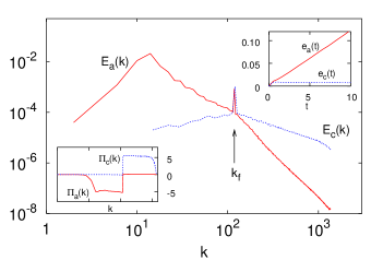
Figure 3: Power spectra of active (red) and passive (blue) scalar variances $E_{a}(k)=\pi k|\hat{a}({\bm{k}},t)|^{2}$ and $E_{c}(k)=\pi k|\hat{c}({\bm{k}},t)|^{2}$. In the lower left corner, the fluxes of scalar variance $\Pi_{a,c}$ out of wavenumber $k$. Negative values indicate an inverse cascade. In the upper right corner, the total scalar variance $e_{a,c}(t)=\int E_{a,c}(k,t)\,dk$. The active variance $e_{a}(t)$ grows linearly in time whereas $e_{c}(t)$ fluctuates around a finite value (see text). The rate of active to passive scalar dissipation is $\epsilon_{a}/\epsilon_{c}\simeq 0.005$. All fields are set to zero at $t=0$, and time is defined in units of eddy-turnover time ${\cal T}=l_{f}/v_{\mathrm{rms}}$ where $l_{f}=2\pi/k_{f}$. At $k<k_{f}$ we observe power-law behaviors $E_{a}(k)\sim k^{-2.0\pm 0.1}$ and $E_{c}(k)\sim k^{0.7\pm 0.1}$, while at $k>k_{f}$ we find $E_{a}(k)\sim k^{-3.6\pm 0.1}$ and $E_{c}(k)\sim k^{-1.4\pm 0.1}$.

Eqs. (25) and (26) have two quadratic invariants in the inviscid and unforced limit, namely the total energy ${1\over 2}\int(v^{2}+b^{2}){\rm d}{\bm{x}}$ and the mean square magnetic potential ${1\over 2}\int a^{2}{\rm d}{\bm{x}}$. Using standard quasi-equilibrium arguments [6], an inverse cascade of magnetic potential is expected to take place in the forced and dissipated case [43]. This expectation has been confirmed in numerical experiments [45]. Let us now compare the magnetic potential with a passive scalar evolving in the same flow.

We performed a high-resolution ($4096^{2}$ collocation points) direct numerical simulations of Eqs. (25)-(26) along with a passive scalar (2). The scalar forcing terms $f_{a}$ and $f_{c}$ are homogeneous independent Gaussian processes with zero mean and correlation

$$\langle\hat{f}_{i}({\bm{k}},t)\hat{f}_{j}({\bm{k}}^{\prime},t^{\prime})\rangle={F_{0}\over(2\pi k_{f})}\delta_{ij}\delta({\bm{k}}+{\bm{k}}^{\prime})\delta(k-k_{f})\delta(t-t^{\prime})$$ (27)

where $i,j=a,c$. The injection length scale $l_{f}\sim 2\pi/k_{f}$ has been chosen roughly in the middle of the available range of scales. $F_{0}$ is the rate of scalar variance input.

In Fig. 3 we summarize the spectral properties of the two scalars. The emerging picture is as follows. While $a$ undergoes an inverse cascade process, $c$ cascades downscale. This striking difference is reflected in the behavior of the dissipation. The active scalar dissipation, $\epsilon_{a}=\kappa|{\bm{\nabla}a}|^{2}$, vanishes in the limit $\kappa\to 0$ – no dissipative anomaly for the field $a$. Consequently, the squared magnetic potential grows linearly in time $e_{a}(t)={1\over 2}\int a^{2}d{\bm{x}}\approx{1\over 2}F_{0}t$. On the contrary, for the passive scalar, a dissipative anomaly is present and $\epsilon_{c}=\kappa|{\bm{\nabla}c}|^{2}$ equals the input ${1\over 2}F_{0}$ holding $c$ in a statistically stationary state. (See inset in Fig. 3).

Figure 4: Velocity power spectrum $E_{v}(k)=\pi k|\hat{v}({\bm{k}},t)|^{2}$. For $k<k_{f}$, in agreement with previous simulations [45], we observe $E_{v}(k)\sim k^{1/3}$ (dashed lines) which deviates from the dimensional prediction $k^{-1/3}$. In the range $k>k_{f}$ a scaling close to $k^{-5/3}$ is observed, indicating that ${\bm{v}}$ is rough both in the inverse and in the direct cascade range.

The velocity field is rough (as confirmed by its spectrum, see Fig. 4) and incompressible, therefore particle paths are not unique and explosively separate. This entails the dissipative anomaly for passive scalars. On the contrary, the dissipative anomaly is absent for the magnetic potential, in spite of the fact that the trajectories are the same – the advecting velocity is the same. How can these two seemingly contradictory statements be reconciled ?

4.2 Dissipative anomaly and particle paths

The solution of the riddle resides in the relationship between the Lagrangian trajectories and the active scalar input $f_{a}$. These two quantities are bridged by the Lorentz force appearing in (26). To study the correlations between forcing and particle paths we need to compute the evolution of the particle propagator. The relevant observables are the time sequences of $\phi_{a,c}(s)=\int d{\bm{y}}\,f_{a,c}({\bm{y}},s)P({\bm{y}},s|{\bm{x}},t)$. Indeed the equivalent of Eq. (12) can be written for the active scalar as

$$a({\bm{x}},t)=\int_{0}^{t}ds\int d{\bm{y}}\,f_{a}({\bm{y}},s)P({\bm{y}},s|{\bm{x}},t)\;.$$ (28)

The main difficulty encountered here is that $P$ evolves backward in time according to (10) and the condition $P({\bm{y}},t|{\bm{x}},t)=\delta({\bm{y}}-{\bm{x}})$ is set at the final time $t$. Conversely, the initial conditions on velocity and scalar fields are set at the initial time. The solution of this mixed initial/final value problem is a non-trivial numerical task. To this aim, we devised a fast and low-memory demanding algorithm to integrate Eqs. (25) - (26) and (10) with the appropriate initial/final conditions. The details are given in Ref. [44].

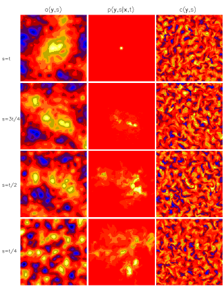
Figure 5: Time runs from bottom to top. First column: time evolution of the active scalar field resulting from the numerical integration of Eqs. (25) and (26). Second column: backward evolution of the particle propagator according to Eq. (10). Third column: time evolution of the passive scalar field in the same flow.

The typical evolution of the propagator is shown in the central column of Fig. 5. From its evolution we reconstructed the time sequences of the forcing contributions $\phi_{a,c}(s)$ which, integrated over $s$, give the amplitude of the scalar fields according to (12) and (28). The time series of $\phi_{a}(s)$ and $\phi_{c}(s)$ are markedly different (Fig. 6), the former being strongly skewed toward positive values at all times. This signals that trajectories preferentially select regions where $f_{a}$ has a positive sign, summing up forcing contributions to generate a typical variance of $a$ of the order $F_{0}t$. On the contrary, the passive scalar sequence displays the usual features: $f_{c}$ is independent of $P$ and their product can be positive or negative with equal probability on distant trajectories. This ensures that the time integral in Eq. (12) averages out to zero for $|s-t|>{\cal T}_{\ell_{f}}$ (see Sect. 2.2) and yields $c^{2}\sim F_{0}{\cal T}_{\ell_{f}}$.

As shown in the lower panel of Fig. 6 the effect of correlations between forcing and propagator is even more striking comparing $\int_{0}^{s}{\rm d}s^{\prime}\phi_{a}(s^{\prime})$ with $\int_{0}^{s}{\rm d}s^{\prime}\phi_{c}(s^{\prime})$. The conspicuous difference has to be related to a strong spatial correlation between $P$ and $a$, as can be inferred from

$$\int_{0}^{s}\phi_{a}(s^{\prime})\,ds^{\prime}=\int d{\bm{y}}\,a({\bm{y}},s)P({\bm{y}},s|{\bm{x}},t)\,,$$ (29)

which can be derived from (25) and (11). An equivalent relation holds for $c$ as well. The comparison of the first and the second column of Fig. 5 highlights the role of spatial correlations: the distribution of particles follows the distribution of the active scalar. This amounts to saying that large-scale scalar structures are built out of smaller ones that coalesce together [45]. This has to be contrasted with the absence of large-scale correlations between the propagator and the passive scalar field (second and third column of Fig. 5).

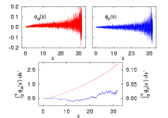
Figure 6: Top: $\phi_{a,c}(s)=\int d{\bm{y}}\,f_{a,c}({\bm{y}},s)P({\bm{y}},s|{\bm{x}},t)$. The two graphs have the same scale on the vertical axis. Here, $t=32$. Bottom: time integrals $\int_{0}^{s}\phi_{a}(s^{\prime})\,ds^{\prime}$ (upper curve) and $\int_{0}^{s}\phi_{c}(s^{\prime})\,ds^{\prime}$ (lower curve). Note the different scale on the vertical axis. Recall that $\int_{0}^{t}\phi_{a}(s^{\prime})\,ds^{\prime}=a({\bm{x}},t)$ (and similarly for $c$).

Let us now clarify the mechanism for the absence of dissipative anomaly. Consider the squared active field $a^{2}$. It can be expressed in two equivalent ways. On one hand, it can be written as the square of (28). On the other hand, multiplying (25) by $2a$ one obtains the equation

$$\partial_{t}a^{2}+{\bm{v}}\cdot\nabla a^{2}=\kappa\Delta a^{2}+2af_{a}-2\epsilon_{a}\,.$$ (30)

Exploiting the absence of dissipative anomaly, $\epsilon_{a}=0$, Eq. (30) reduces to a transport equation that can be solved in terms of particle trajectories. The comparison of the two expressions yields [46]

$$\int_{0}^{t}ds\int_{0}^{t}ds^{\prime}\int\int f_{a}({\bm{y}},s)f_{a}({\bm{y}}^{\prime},s^{\prime})P({\bm{y}},s|{\bm{x}},t)P({\bm{y}}^{\prime},s^{\prime}|{\bm{x}},t) =$$

$$\int_{0}^{t}ds\int_{0}^{t}ds^{\prime}\int\int f_{a}({\bm{y}},s)f_{a}({\bm{y}}^{\prime},s^{\prime})P({\bm{y}}^{\prime},s^{\prime};{\bm{y}},s|{\bm{x}},t)\,,$$ (31)

where $P({\bm{y}}^{\prime},s^{\prime};{\bm{y}},s|{\bm{x}},t)=P({\bm{y}},s|{\bm{x}},t)P({\bm{y}}^{\prime},s^{\prime}|{\bm{y}},s)$ denotes the probability that a trajectory ending in $({\bm{x}},t)$ were in $({\bm{y}},s)$ and $({\bm{y}}^{\prime},s^{\prime})$. Integration over ${\bm{y}}$ and ${\bm{y}}^{\prime}$ is implied. Eq. (31) amounts to saying that

$$\left\langle\int_{0}^{t}f_{a}({\bm{\rho}}(s),s)ds\right\rangle_{\bm{w}}^{2}\!\!=\!\left\langle\left[\int_{0}^{t}f_{a}({\bm{\rho}}(s),s)ds\right]^{2}\right\rangle_{\bm{w}}\,,$$ (32)

meaning that $\int_{0}^{t}f_{a}({\bm{\rho}}(s),s)ds$ is a non-random variable over the ensemble of trajectories. The above procedure can be generalized to show that $\langle\int_{0}^{t}f_{a}({\bm{\rho}}(s),s)ds\rangle_{\bm{w}}^{N}=\langle[\int_{0}^{t}f_{a}({\bm{\rho}}(s),s)ds]^{N}\rangle_{\bm{w}}$.

In plain words, the absence of the dissipative anomaly is equivalent to the property that along any of the infinite trajectories ${\bm{\rho}}(s)$ ending in $({\bm{x}},t)$ the quantity $\int_{0}^{t}f_{a}({\bm{\rho}}(s),s)ds$ is exactly the same, and equals $a({\bm{x}},t)$. Therefore, a single trajectory suffices to obtain the value of $a({\bm{x}},t)$, contrary to the passive case where different trajectories contribute disparate values of $\int_{0}^{t}f_{c}({\bm{\rho}}(s),s)ds$, with a typical spread $\epsilon_{c}t$, and only the average over all trajectories yields the correct value of $c({\bm{x}},t)$. In the unforced case particles move along isoscalar lines: this is how non-uniqueness and explosive separation of trajectories is reconciled with the absence of dissipative anomaly.

Inverse cascades appear also for passive scalars in compressible flows [34]. There, the ensemble of the trajectories collapses onto a unique path, fulfilling in the simplest way the constraint (31). In MHD the constraint is satisfied thanks to the subtle correlation between forcing and trajectories peculiar to the active case.

Magnetohydrodynamics in two dimension represents an “extreme” example of the effect of correlations among Lagrangian paths and the active scalar input. The property that all trajectories ending in the same point should contribute the same value of the input poses a global constraint over the possible paths.

Before discussing the statistical properties of $a$, on the basis of the previous discussion it is instructive to reconsider the concept of dissipative anomaly in general scalar turbulence.

4.3 Dissipative anomaly revisited

In this subsection we give an alternative interpretation of dissipative anomaly. To this aim, let us denote with $\Theta({\bm{x}},t)$ a generic scalar field, regardless of its passive or active character. The scalar evolves according to the transport equation

$$\partial_{t}\Theta+{\bm{v}}\cdot{\bm{\nabla}}\Theta=\kappa\Delta\Theta+f_{\Theta}\,.$$ (33)

We can formally solve Eq. (33) by the method of characteristics, i.e. in terms of the stochastic ordinary differential equations

$${{\rm d}{\bm{\rho}}(t)\over{\rm d}t} = {\bm{v}}({\bm{\rho}}(t),t)+\sqrt{2\kappa}\dot{\bm{w}},$$ (34)

$${{\rm d}\vartheta(t)\over{\rm d}t} = f_{\Theta}({\bm{\rho}}(t),t)\,.$$ (35)

At variance with the procedure adopted in Sect. 2.2 here we are not conditioning a priori the paths to their final positions. The Eulerian value of the field is recovered once the average over the all paths, ${\bm{\rho}}$, landing in $({\bm{x}},t)$ is performed, i.e. $\Theta({\bm{x}},t)=\langle\vartheta(t)\rangle_{\bm{w}}$. Recall that if the flow is non-Lipschitz continuous, such paths do not collapse onto a single one also for $\kappa\to 0$.

We can now define $P({\bm{x}},\vartheta,t|{\bm{x}}_{0},\vartheta_{0},0)$ as the probability that a path which started in ${\bm{x}}_{0}$ at time $0$ with $\vartheta_{0}=\Theta({\bm{x}}_{0},0)$ and arrives in ${\bm{x}}$ at time $t$ carrying a scalar value $\vartheta$. Notice that the conditioning is now on the initial value, and $P$ evolves according to the Kolmogorov equation:

$$\partial_{t}P+{\bm{v}}\cdot{\bm{\nabla}}_{\bm{x}}P+f_{\Theta}\nabla_{\vartheta}P=\kappa\Delta P$$ (36)

with initial condition $P({\bm{x}},\vartheta,t|{\bm{x}}_{0},\vartheta_{0},0)=\delta({\bm{x}}-{\bm{x}}_{0})\delta(\vartheta-\vartheta_{0})$ and $\vartheta_{0}=\Theta({\bm{x}},0)$.

Figure 7: $\int{\rm d}{\bm{x}}\,\sigma^{2}_{a}({\bm{x}},t)$ (boxes) and $\int{\rm d}{\bm{x}}\,\sigma^{2}_{c}({\bm{x}},t)$ (circles) vs time. We have integrated Eqs. (25) and (2) for two different values of the diffusivity $\kappa=0.003$ (filled symbols) at resolution $512^{2}$ and $\kappa=0.001$ (open symbols) at resolution $1024^{2}$. The straight lines indicates the growth laws $2\epsilon_{a}t$ and $2\epsilon_{c}t$ for the two values of $\kappa$. Note that $\epsilon_{c}$ does not depend on $\kappa$ consistently with the presence of dissipative anomaly, while $\epsilon_{a}$ decreases as $\kappa$ decreases. The variance has been evaluated averaging over $10^{6}$ Lagrangian paths evolving according to (34). The Lagrangian scalar values $\vartheta_{a}$ and $\vartheta_{c}$ (where $a({\bm{x}},t)=\int\vartheta_{a}{\cal P}({\bm{x}},\vartheta_{a},t){\rm d}\vartheta_{a}$, the equivalent relation holds between $c$ and $\vartheta_{c}$) have been computed integrating (35) both for the active $f_{a}$ and passive $f_{c}$ forcings along each paths. The forcings are chosen as in (27) The initial Eulerian $a({\bm{x}},0)$, $c({\bm{x}},0)$ and Lagrangian $\vartheta_{a}(0)$, $\vartheta_{c}(0)$ fields have been set to zero. Times is measured in eddy turnover times.

Integrating over the initial conditions we define now the probability density ${\cal P}({\bm{x}},\vartheta,t)=\int P({\bm{x}},\vartheta,t|{\bm{x}}_{0},\Theta({\bm{x}}_{0},0),0){\rm d}{\bm{x}}_{0}$. ${\cal P}$ still obeys to (36) with initial condition ${\cal P}({\bm{x}},\vartheta,0)\!=\!\delta(\vartheta-\Theta({\bm{x}}_{0},0))$, and represents the probability that a path arrives in $({\bm{x}},t)$ carrying a scalar value $\vartheta(t)\!=\!\int_{0}^{t}f_{\Theta}(\rho(s),s){\rm d}s$.

Let us now look at the variance of the distribution of such values, i.e. $\sigma^{2}_{\Theta}({\bm{x}},t)\!=\!\int\vartheta^{2}{\cal P}{\rm d}\vartheta-(\int\vartheta{\cal P}{\rm d}\vartheta)^{2}$. From Eq. (36) it is easy to derive the following equation

$$\partial_{t}\sigma^{2}_{\Theta}({\bm{x}},t)\!+\!{\bm{v}}\cdot\!{\bm{\nabla}}_{\bm{x}}\sigma^{2}_{\Theta}({\bm{x}},t)\!=\!\kappa\Delta\sigma^{2}_{\Theta}({\bm{x}},t)\!+\!2\epsilon_{\Theta}({\bm{x}},t)$$ (37)

where $\epsilon_{\Theta}({\bm{x}},t)=\kappa|{\bm{\nabla}}_{\bm{x}}\int\vartheta{\cal P}({\bm{x}},\vartheta,t){\rm d}\vartheta|^{2}$. In the Eulerian frame $\epsilon_{\Theta}({\bm{x}},t)=\kappa|{\bf\nabla}\Theta({\bm{x}},t)|^{2}$, i.e. the local dissipation field.

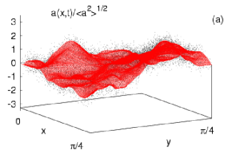
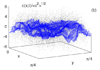
Figure 8: (a) The surface is the instantaneous Eulerian magnetic potential field $a({\bm{x}},t)$. The dots represent the positions of particles in the $({\bm{x}},\vartheta_{a})$-space at time $t$. (b) The same for the passive scalar, $c$. The time $t$ corresponds to the largest time in Fig. 7. For visualization purposes only the portion $[0,\pi/4]\times[0,\pi/4]$ is displayed. In (a) the cloud of dots closely follows the the magnetic potential surface, while in (b) they are considerably more dispersed (notice the differences in the values of the $\vartheta$-axis).

Integrating over ${\bm{x}}$, we end up with

$${{\rm d}\over{\rm d}t}\int\sigma^{2}_{\Theta}({\bm{x}},t){\rm d}{\bm{x}}=2\int\epsilon_{\Theta}({\bm{x}},t){\rm d}{\bm{x}}=2\epsilon_{\Theta}\,,$$ (38)

where $\epsilon_{\Theta}=\langle\kappa|{\bf\nabla}\Theta({\bm{x}},t)|^{2}\rangle$ is the average dissipation rate of $\langle\Theta^{2}\rangle/2$. Therefore, if $\Theta^{2}$ cascades toward the small scales with a finite (even in the limit $\kappa\to 0$) dissipation, $\epsilon_{\Theta}$, the variance of the distribution of the values of $\vartheta(t)=\int_{0}^{t}{\rm d}sf_{\Theta}({\bm{\rho}}(s),s)$ will grow linearly in time. Conversely, for an inverse cascade of $\Theta^{2}$ in the absence of dissipative anomaly $\int{\rm d}{\bm{x}}\sigma^{2}_{\Theta}({\bm{x}},t)=0$, corresponding to a singular distribution ${\cal P}({\bm{x}},\vartheta,t)=\delta(\vartheta-\Theta({\bm{x}},t))$.

In Fig. 7 we show the time evolution of $\int{\rm d}{\bm{x}}\,\sigma^{2}_{a,c}({\bm{x}},t)$ in the case of $2d$ MHD which confirms the above findings.

The fact that, for inverse cascading scalars, the probability density ${\cal P}$ collapses onto a $\delta$-function in the limit of vanishing diffusivity amounts to saying that particles in the $({\bm{x},\vartheta})$ space do not disperse in the $\vartheta$-direction but move remaining attached to the surface $\vartheta=\Theta({\bm{x}},t)$. (see Fig. 8a). This is related to the strong spatial correlations between $a$ and the Lagrangian propagator observed in Fig. 5. On the contrary, for a direct cascade of scalar such correlations do not exist and dissipation takes place because of dispersion in the $\vartheta$-direction (see Fig. 8b).

4.4 Eulerian statistics

4.4.1 Single-point statistics

The statistical properties of the magnetic potential $a$ and the passive scalar $c$ are markedly different already at the level of the single-point statistics. The pdf of $a$ is Gaussian, with zero mean and variance $F_{0}t$ (Fig. 9). Conversely, the pdf of $c$ is stationary and supergaussian (see Fig. 9), as it generically happens for passive fields sustained by a Gaussian forcing in rough flows [27].

The Gaussianity of the pdf of $a$ is a straightforward consequence of the vanishing of active scalar dissipation. This is simply derived by multiplying Eq. (25) for $2na^{2n-1}$ and averaging over the forcing statistics. The active scalar moments obey the equation $\partial_{t}\langle a^{2n}\rangle=n(2n-1)F_{0}\langle a^{2n-2}\rangle$ (odd moments vanish by symmetry) whose solutions are the Gaussian moments: $\langle a^{2n}\rangle=(2n-1)!!(F_{0}t)^{n}$.

Figure 9: Pdf’s of active (empty boxes) and passive (full boxes) scalar fields normalized by their standard deviation. The active scalar pdf is indistinguishable from a Gaussian (solid line).

An equivalent derivation can be obtained in Lagrangian terms. Following the same steps which lead from Eq. (30) to (31) it is easy to derive the following expression

$$a^{2n}({\bm{x}},t)\!=\!2n\!\!\!\int_{0}^{t}\!\!{\rm d}s_{1}\!\!\int\!\!{\rm d}{\bm{y}}_{1}P({\bm{y}}_{1},s_{1}|{\bm{x}},t)f_{a}({\bm{y}}_{1},s_{1})a^{2n-1}({\bm{y}}_{1},s_{1})\,,$$ (39)

which after integrating over ${\bm{x}}$ and averaging over the forcing statistics reduces to

$$\langle a^{2n}\rangle(t)=n(2n\!-\!1)F_{0}\int_{0}^{t}{\rm d}s\langle a^{2n\!-\!2}\rangle(s)\,,$$ (40)

which, unraveling the hierarchy, yields Gaussian moments written above. In passing from Eq. (39) to (40) we used the property that $\int{\rm d}{\bm{x}}P({\bm{y}},s|{\bm{x}},t)=1$ (which is ensured by Eq. (10)), and Gaussian integration by parts.

4.4.2 Multi-point statistics and the absence of anomalous scaling in the inverse cascade

The results about two-point statistics of the magnetic potential and passive scalar fields is summarized in Fig. 10. In the inverse cascade scaling range $r>\ell_{f}$ the rescaled pdf of $\delta_{r}a$ at different values of the separation $r$ collapse onto the same curve indicating absence of anomalous scaling (Fig. 10a). By contrast, in the scaling range $r<\ell_{f}$ the rescaled pdfs of passive scalar increments at different $r$ do not collapse (Fig. 10b), i.e. we have anomalous scaling, as expected.

Figure 10: (a) Rescaled pdf of the normalized active scalar increments, $\delta_{r}a/\langle(\delta_{r}a)^{2}\rangle^{1/2}$, for three separations in the $r>\ell_{f}$ range: $r=2\ell_{f}$ ($\times$) ,$3\ell_{f}$ ($\circ$), $4\ell_{f}$ ($\Box$). The normalized passive scalar increments pdf at the same scales (dashed line) and the Gaussian (solid line) are shown for comparison . In the inset the rescaled pdf of $\delta_{r}a$ for $r=3\ell_{f}$ (solid line) is shown in the interval $[-2.5:2.5]$ in linear scale, to emphasize the deviation from a Gaussian (dashed line). The flatness is $\approx 2.76$, significantly smaller than the Gaussian value $3$. (b) Rescaled pdf of the passive scalar increments, $\delta_{r}c/\langle(\delta_{r}c)^{2}\rangle^{1/2}$, for two separations in the $r<\ell_{f}$ range: $r=0.3\ell_{f}$ (full triangles) and $0.6\ell_{f}$ ($\Box$). The rescaled pdfs of active scalar increments at the same scales (solid line) and a Gaussian (dashed line) are reported for comparison.

Let us now consider in quantitative terms the scaling behaviors. Since in our simulations the scaling range at $r<\ell_{f}$ ($k>k_{f}$) is poorly resolved, we do not enter the much debated issue of the scaling of the magnetic and velocity fields in this range of scales (see, e.g., [45, 43, 47, 48, 49, 50]). We just mention that current opinions are divided between the Kolmogorov scaling $\delta_{r}v\sim r^{1/3}$, and the Iroshnikov-Kraichnan $\delta_{r}v\sim r^{1/4}$, corresponding to spectral behaviors such as $E_{v}(k)\sim k^{-5/3}$ and $E_{v}(k)\sim k^{-3/2}$, respectively. Both theories agree on the smooth scaling behavior for the magnetic potential, $\delta_{r}a\sim r$, that is observed numerically (see Fig. 3). In the range of scales $r>\ell_{f}$ ($k<k_{f}$) standard dimensional arguments predict $E_{a}(k)\sim k^{-7/3}$ [6, 43, 45], which is different from our findings $E_{a}(k)\sim k^{-2}$ (Fig. 11). In real space this means that $\delta_{r}a\sim r^{1/2}$, which is dimensionally compatible with scaling behavior $\delta_{r}v=[{\bm{v}}({\bm{x}}+{\bm{r}},t)-{\bm{v}}({\bm{x}},t)]\cdot{\hat{\bm{r}}}\sim r^{0}$ for $r>\ell_{f}$ (as suggested by the velocity spectrum, see Fig. 4), and the Yaglom relation $\langle\delta_{r}v(\delta_{r}a)^{2}\rangle\simeq F_{0}r$ [4]. As a side remark, note that the argument for $E_{a}(k)\sim k^{-7/3}$ rests on the assumption of locality for velocity increments, a hypothesis incompatible with the observed velocity spectrum at $k<k_{f}$ (see Fig. 4).

It is worth remarking that the increments of active scalar $\delta_{r}a=a({\bm{x}}+{\bm{r}},t)-a({\bm{x}},t)$ eventually reach a stationary state in spite of the growth of $a^{2}$. The distribution of of $\delta_{r}a$ is subgaussian (Fig. 10). This behaviour can be explained recalling that $\delta_{r}a$ is the difference of two Gaussian variables, which are however strongly correlated (indeed the main contributions will come from ${\bm{x}}+{\bm{r}}$ and ${\bm{x}}$ inside the same island, see Fig. 5). This correlation leads to cancellations resulting in the observed subgaussian probability density function.

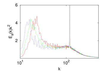
Figure 11: Compensated power spectra of active scalar variances $E_{a}(k)k^{2}$ at three different times of the evolution. Note that an increasingly clear plateau at $k<k_{f}$ appears.

Let us now focus on the most interesting aspect, namely the absence of anomalous scaling in the inverse cascade range. The absence of intermittency seems to be a common feature of inverse cascading systems as passive scalars in compressible flows [34, 33] and the velocity field in two dimensional Navier Stokes turbulence [42]. This leads to the conjecture that an universal mechanism may be responsible for the self similarity of inverse cascading systems. While $2d$ Navier-Stokes turbulence is still far to be understood, the absence of anomalous scaling in passive scalars evolving in compressible flows has been recently understood in terms of the collapse of the Lagrangian trajectories onto a unique path [33, 34]. Briefly, the collapse of trajectories allows to express the $2N$-order structure function in terms of two-particle propagators, $\langle P_{2}\rangle_{v}$, instead of the $2N$-particle propagator, $\langle P_{2N}\rangle_{v}$. While the latter may be dominated by a zero mode with a non trivial anomalous scaling, the former are not anomalous and lead to dimensional scaling.

The above argument cannot be simply exported to the magnetic potential inverse cascade: first, the Lagrangian paths do not collapse onto a unique one; second, the correlation between the $f_{a}$ and ${\bm{v}}$ does not allow to split the averages. However, the former difficulty can be overcome. Indeed the property that all paths landing in the same point contribute the same value has important consequences also in the multipoints statistics. Proceeding as for the derivation of Eq. (31), it is possible to show that $m$ trajectories are enough to calculate the product of arbitrary powers of $a$ at $m$ different points $\langle a^{n_{1}}({\bm{x}}_{1},t)\dots a^{n_{m}}({\bm{x}}_{m},t)\rangle$. In particular, structure functions $S^{a}_{N}(r)=\langle(\delta_{r}a)^{N}\rangle$ for any order $N$ involve only two trajectories. This should be contrasted with the passive scalar, where the number of trajectories increases with $N$ and this is at the core of anomalous scaling of passive fields [27].

5 Two-dimensional Ekman turbulence

Let us now consider the case of scalars that act on the velocity field through a functional dependence. Among them, probably the best known case is vorticity in two dimensions $a={\bm{\nabla}}\times{\bm{v}}$. It obeys the Ekman-Navier-Stokes equation

$$\partial_{t}a+{\bm{v}}\cdot{\bm{\nabla}}a=\kappa\Delta a-\alpha\,a+f_{a}\,,$$ (41)

The term $-\alpha\,a$ models the Ekman drag experienced by a thin fluid layer with the walls or the surrounding air [7, 37].

In the absence of friction ($\alpha=0$) dimensional arguments [51, 52], confirmed by experiments [41, 53] and numerical simulations [42], give the following scenario. At large scales an inverse (non-intermittent) cascade of kinetic energy takes place with $E_{v}(k)\sim k^{-5/3}$ and $E_{a}(k)\sim k^{1/3}$. At small scales the enstrophy, $\langle a^{2}\rangle$, performs a forward cascade with $E_{a}(k)\sim k^{-1}$ and $E_{v}(k)\sim k^{-3}$, meaning that the velocity field is smooth in this range of scales.

In the presence of friction ($\alpha>0$) kinetic energy is removed at large scales holding the system in a statistically steady state and small-scale statistics is modified by the competition of the inertial (${\bm{v}}\cdot{\bm{\nabla}}a$) and friction ($-\alpha\,a$). Since these two terms have the same dimension due to smoothness of the velocity field, this results in nontrivial scaling laws for $a$. This effect is evident in DNS with $\alpha>0$ [17, 12], where the vorticity spectrum displays a power law steeper than in the frictionless case: $E_{a}(k)\sim k^{-1-\xi}$ with $\xi$ dependent on $\alpha$ (see Fig. 12a). For $0<\xi<2$ the exponent $\xi$ coincides with the scaling exponent, $\zeta^{a}_{2}$, of the second order structure function $S^{a}_{2}(r)$. Additionally, high-order structure functions at fixed $\alpha$ show anomalous scaling, $\zeta^{a}_{N}\neq N\xi/2$ [12].

Figure 12: (a)The vorticity spectrum $E_{a}(k)\sim k^{-1-\xi}$ steepens by increasing the Ekman coefficient $\alpha$. Here $\alpha=0.15$ $(+)$, $\alpha=0.23$ $(\times)$, $\alpha=0.30$ $(\odot)$. In the inset, the exponent $\xi$ as a function of $\alpha$. (b) Power spectra of passive scalar ($\times$) and vorticity ($+$). Here $\alpha=0.15$. In the inset we show the same spectra compensated by $k^{1+\zeta^{c}_{2}}$. For details on the DNS see [12].

The spectral steepening and the presence of intermittency are observed [16, 12] also in passive scalars evolving in smooth flows according to

$$\partial_{t}c+{\bm{v}}\cdot{\bm{\nabla}}c=\kappa\Delta c-\alpha\,c+f_{c}\,$$ (42)

Physically Eq. (42) describes the evolution of a decaying passive substance (e.g. a radioactive marker) [4, 54]. For $\alpha=0$ the dimensional expectation $E_{c}(k)\sim k^{-1}$ has been verified in experiments [55]. For positive $\alpha$ passive scalar spectra become steeper than $k^{-1}$ and, at high wavenumbers, have the same slope of the vorticity spectrum (Fig. 12b). Additionally, the pdfs of passive and vorticity increments for separations inside the inertial range collapse one onto the others (Fig. 13), signalling that the scaling exponents coincide: $\zeta^{c}_{N}=\zeta^{a}_{N}$. In summary, the vorticity field and the passive scalar share the same statistical scaling properties [17, 16, 12], similarly to the 2D convection case. However, differences may appear for odd order moments [56].

It is now interesting to understand how the equivalence of active and passive statistics is realized: we shall see that in this case the smoothness of the flow is a crucial ingredient.

Figure 13: Probability density functions of vorticity differences ($+$) and of passive scalar ones ($\times$), normalized by their respective standard deviation, at different scales $r$ within the scaling range.

Let us start with the decaying passive scalar (42). First of all, it should be noted that the presence of non-zero friction ($\alpha>0$) regularizes the field, and there is absence of dissipative anomaly [54], even if the mechanism is different from the MHD one. As a consequence, in Eq. (42) we can put $\kappa=0$ and solve it by the method of characteristics (see Sect. 2.2), i.e. $c({\bm{x}},t)=\int_{-\infty}^{t}{\rm d}sf_{c}({\bm{\rho}}(s;{\bm{x}},t),s)\exp(-\alpha(t-s))$, where now the path ${\bm{\rho}}(s;{\bm{x}},t),s)$ is unique due to the smoothness of the velocity field (note that $E_{v}(k)\sim k^{-3-\xi}$ is always steeper than $k^{-3}$, see also Fig. 12a). The integral extends up to $-\infty$ where the initial conditions are set.

Passive scalar increments $\delta_{r}c=c({\bm{x}}_{1},t)-c({\bm{x}}_{2},t)$ ($r=|{\bm{x}}_{1}-{\bm{x}}_{2}|$), which are the objects we are interested in, are associated to particles pairs

$$\delta_{r}c=\!\!\!\int_{-\infty}^{t}\!\!\!{\rm d}se^{-\alpha(t-s)}[f_{c}({\bm{\rho}}(s;{\bm{x}}_{1},\!t),s)\!-\!\!f_{c}({\bm{\rho}}(s;{\bm{x}}_{2},\!t),s)]\,.$$ (43)

It should be now noted that the integrand $f_{c}({\bm{\rho}}(s;{\bm{x}}_{1},\!t),s)\!-\!\!f_{c}({\bm{\rho}}(s;{\bm{x}}_{2},\!t),s)$ stays small as long as the separation between the two paths remains below the forcing correlation scale, $\ell_{f}$; while for separations larger than $\ell_{f}$ it is approximately equal to a Gaussian random variable, $X$. In the latter statement we used the independence between $f_{c}$ and the particle trajectories, ensured by the passive nature of $c$. Therefore, Eq. (43) can be approximated as

$$\delta_{r}c\approx X\int_{-\infty}^{t-{\cal T}_{\ell_{f}}(r)}\!\!{\rm d}s\,e^{-\alpha(t-s)}\sim Xe^{-\alpha{\cal T}_{\ell_{f}}(r)}\,,$$ (44)

where ${\cal T}_{\ell_{f}}(r)$ is the time necessary for the particles pair to go from $r$ to $\ell_{f}$ backward in time. It is now clear that large fluctuations are associated to fast separating couples, ${\cal T}_{\ell_{f}}(r)\ll\langle{\cal T}_{\ell_{f}}(r)\rangle$, and small fluctuations to slow ones. Moreover, since ${\bm{v}}$ is smooth, two-dimensional and incompressible pairs separation is exponential and its statistics is described by a single finite-time Lyapunov exponent [57], $\gamma$. It is related to the separation time through the relation:

$$\ell_{f}=re^{\gamma{\cal T}_{\ell_{f}}(r)}\,.$$ (45)

Large deviations theory states that at large times the random variable $\gamma$ is distributed as $P(\gamma,t)\sim t^{1/2}\exp[-S(\gamma)t]$. $S(\gamma)$, the so-called Cramer function [58], is positive, concave and has a quadratic minimum, $S(\lambda)=0$ in $\lambda$, the maximum Lyapunov exponent. From (44) and (45) along with with the expression for $P(\gamma,t)$, structure functions can be computed as

$$S^{c}_{N}(r)\sim\langle X^{N}\rangle\int{\rm d}\gamma\left({r\over\ell_{f}}\right)^{{N\alpha+S(\gamma)\over\gamma}}\approx\left({r\over\ell_{f}}\right)^{\zeta^{c}_{N}}\,,$$ (46)

where $\zeta^{c}_{N}=\min_{\gamma}\{N,[N\alpha+S(\gamma)]/\gamma\}$. Fig. 14 shows that this prediction is verified by numerical simulations. The anomalous exponents $\zeta^{c}_{N}$ can therefore be evaluated in terms of the flow properties through the Cramér funtion $S(\gamma)$.

Figure 14: The scaling exponents of the passive scalar $\zeta^{c}_{p}$ ($+$), which have been computed also for noninteger moments, indeed Eq. (46) holds in general. We also show the exponents obtained from the separation times statistics ($\odot$) according to $\langle\exp[-\alpha p{\cal T}_{\ell_{f}}(r)]\rangle\sim r^{\zeta_{p}^{c}}$ with average over about $2\times 10^{5}$ couple of Lagrangian particles. The errorbars are estimated by the r.m.s. fluctuation of the local slope. In the inset we plot the Cramer function $S(\gamma)$ computed from finite time Lyapunov exponents (symbols) and exit time statistics (line).

Since $\zeta^{c}_{N}=\zeta^{a}_{N}$ one may be tempted to apply straightforwardly to vorticity the same argument used for the passive scalar. However, the crucial assumption used in the derivation of Eq. (46) is the statistical independence of particle trajectories and the forcing. That allows to consider ${\cal T}_{\ell_{f}}(r)$ and $X$ as independent random variables. While this is obviously true for $c$, it is clear that the vorticity forcing, $f_{a}$, may influence the velocity statistics and, as a consequence, the particle paths. In other terms, for the vorticity field we cannot a priori consider $X$ and ${\cal T}_{\ell_{f}}(r)$ as independent.

Nevertheless, it is possible to argue in favour of the validity of Eq. (43) also for vorticity. Indeed, the random variable ${\cal T}_{\ell_{f}}(r)$ is essentially determined by the evolution of the strain along the Lagrangian paths for times $t-{\cal T}_{\ell_{f}}(r)<s<t$, whilst $X$ results from the scalar input accumulated at times $s<t-{\cal T}_{\ell_{f}}(r)$. Since the strain correlation time is basically $\alpha^{-1}$, for ${\cal T}_{\ell_{f}}(r)\gg\alpha^{-1}$ it is reasonable to assume that ${\cal T}_{\ell_{f}}(r)$ and $X$ are statistically independent. Eq. (45) allows to translate the condition ${\cal T}_{\ell_{f}}(r)\gg\alpha^{-1}$ into $r\ll\ell_{f}\exp(-\gamma/\alpha)$, and to conlcude that at small scales we can safely assume that the vorticity behaves as a passive field.

We conclude this section with two remarks. First, a difference between the present scenario and the one arisen in two-dimensional convection should be pointed out. Here the scaling exponents depend on the statistics of the finite time Lyapunov exponents, which in turn depends on the way the vorticity is forced. As a consequence universality may be lost. Second, the smoothness of the velocity field plays a central role in the argument used to justify the equivalence of the statistics of $a$ and $c$ in this system. For rough velocity fields ${\cal T}_{\ell_{f}}(r)$ is basically independent of $r$ for $r<<\ell_{f}$ and the argument given in this section would not apply.

6 Turbulence on fluid surfaces

6.1 Surface Quasi Geostrophic turbulence

The study of geophysical fluids is of obvious importance for the understanding of weather dynamics and global circulation. Taking advantage of stratification and rotation, controlled approximations on the Navier-Stokes equations are usually done to obtain more tractable models. For example, the motion of large portions of the atmosphere and ocean have a stable density stratification, i.e. lighter fluid sits above heavier one. This stable stratification, combined with the planetary rotation and the consequent Coriolis force, causes the most energetic motion to occur approximately in horizontal planes and leads to a balance of pressure gradients and inertial forces. This situation is mathematically described by the Quasi-Geostrophic equations [7, 8]. On the lower boundary, the surface of the earth or the bottom of the ocean, the vertical velocity has to be zero and this further simplifies the equations. Assuming that the fluid is infinitely high and that the free surface is flat, the dynamics is then described by the Surface Quasi-Geostrophic equation (SQG) [9, 59]. It governs the temporal variations of the density field, our active scalar $a$ throughout this section. For an ideal fluid the density variation will be proportional to the temperature variation and one can use the potential temperature as fundamental field.

The density fluctuations evolve according to the transport equation

$$\partial_{t}a+{\bm{v}}\cdot{\bm{\nabla}}a=\kappa\Delta a+f_{a}\,,$$ (47)

and the velocity field is functionally related to $a$. In terms of the stream function $\psi$, the density $a$ is obtained as $a({\bm{x}},t)=(-\Delta)^{1/2}\psi({\bm{x}},t)$, and ${\bm{v}}=(\partial_{y},-\partial_{x})\psi$. In Fourier space the link is particularly simple

$$\hat{\bm{v}}({\bm{k}},t)=-i\left({k_{y}\over k},-{k_{x}\over k}\right)\hat{a}({\bm{k}},t)\,.$$ (48)

In the early days of computer simulations eqs. (47) and (48) had been used for weather forecasting. Recently they received renewed interest in view of their formal analogy with the $3d$ Navier-Stokes equations [60, 61], and as a model of active scalar [9, 10]

It is instructive to generalize (48) as

$$\hat{\bm{v}}({\bm{k}},t)=-i\left({k_{y}\over k^{z}},-{k_{x}\over k^{z}}\right)\hat{a}({\bm{k}},t)\,.$$ (49)

For $z=1$ one recovers (48), while $z=2$ corresponds to the $2d$ Navier-Stokes equation and $a$ is the vorticity (see the previous section). The value of $z$ tunes the degree of locality. The case of interest here is $z=1$, corresponding to the same degree of locality as in $3d$ turbulence [9].

Eqs.(47),(49) have two inviscid unforced quadratic invariants $E=-\int{\rm d}{\bm{x}}a\psi$ and $\Omega=\int{\rm d}{\bm{x}}a^{2}$, which for $z=2$ correspond to the energy and the enstrophy, respectively. Notice that, for $z=1$, the fields ${\bm{v}}$ and $a$ have the same dimension and $E_{a}(k)\equiv E_{v}(k)$. Quasi-equilibrium arguments predict an inverse cascade of $E$ and a direct cascade of $\Omega$. If $k_{f}$ identifies the injection wave number dimensional arguments give the expected spectral behavior [9]:

$$E_{a}(k)\propto\left\{\begin{array}[]{cc}k^{-{7\over 3}+{4z\over 3}}\qquad k\ll k_{f}\\ k^{-{7\over 3}+{2z\over 3}}\qquad k\gg k_{f}\end{array}\right.\,.$$ (50)

For $z=2$ one recovers the $2d$ Navier-Stokes expectation [51, 52]. Here, we are interested in the range $k>k_{f}$ and $z=1$, so that $E_{a}(k)\equiv E_{v}(k)\sim k^{-5/3}$ as in $3d$ turbulence. Assuming absence of intermittency, the spectrum $E_{v}(k)\sim k^{-5/3}$ would imply $\delta_{r}v\sim r^{1/3}$. Therefore, for a passive scalar one expects the standard phenomenology: an intermittent direct cascade with $E_{c}(k)\sim k^{-5/3}$ to the Oboukov-Corrsin-Kolmogorov type of arguments [4].

6.1.1 Direct numerical simulations settings

We performed a set of high resolution direct numerical simulations of Eqs. (47) and (48) along with the passive scalar equation (2). Integration has been performed by means of a $2/3$ de-aliased pseudo-spectral method on a $2\pi\times 2\pi$ doubly periodic square domain with ${\cal N}^{2}$ collocation points. Time integration has been done with a second-order Adam-Bashforth or Runge-Kutta algorithms, approriately modified to exactly integrate the dissipative terms. The latter ones, as customary, have been replaced by a hyper-diffusive term that in Fourier space reads $-k^{2p}\hat{a}({\bm{k}},t)$. Since the system is not stationary due to the inverse cascade of $E$, we added an energy sink at large scales in the form $-k^{-q}\hat{a}({\bm{k}},t)$. In order to evaluate its possible effect on inertial quantities, a very high resolution ($4096^{2}$) DNS has been done without any energy sink at large scales.

Table 1: Summary of settings in DNS.

• $\hbox{\phantom{\footnotesize\rm 0}}\hbox{\phantom{\footnotesize\rm 0}}run$	${\cal N}^{2}$	$p$	$q$	$F$	$k_{f}$
  $\hbox{\phantom{\footnotesize\rm 0}}\hbox{\phantom{\footnotesize\rm 0}}1^{a}$	$4096^{2}$	2		B	44-48
  $\hbox{\phantom{\footnotesize\rm 0}}\hbox{\phantom{\footnotesize\rm 0}}2^{b}$	$2048^{2}$	2	1/2	B	2-6
  $\hbox{\phantom{\footnotesize\rm 0}}\hbox{\phantom{\footnotesize\rm 0}}3^{b}$	$2048^{2}$	2	0	G	5
  $\hbox{\phantom{\footnotesize\rm 0}}\hbox{\phantom{\footnotesize\rm 0}}4^{b}$	$2048^{2}$	2	1/2	G	5
  $\hbox{\phantom{\footnotesize\rm 0}}\hbox{\phantom{\footnotesize\rm 0}}5^{c}$	$2048^{2}$	2	0	NG	5

• ^a Runs 1,2 are forced according to Eq. (23), and run 1 is without any friction term.

• ^b Run 3,4 are forced according to Eq. (27).

• ^c Run 5 is forced with the non-Gaussian forcing discussed in Sect. 6.3. Lower ($512^{2}$) resolutions runs with several settings both for the dissipative and friction terms have been also performed

A summary of the numerical settings can be found in table 1. We considered different scalar inputs: (G) a Gaussian $\delta$-correlated in time forcing as (23); (B) a $\delta$-correlated in time one restricted to a few wavenumbers shells as (27); (NG) a non-Gaussian non $\delta$-correlated in time one suited to produce non zero three points correlations for the scalar fields (see below in Sect. 6.3).

6.2 Active and passive scalar statistics in SQG turbulence

Let us start looking at the measured scalar spectra in order to check the dimensional predictions. In Fig. 15 we summarize the spectral behavior for $a$ and $c$ in two different simulations (i.e. runs 1 and 3).

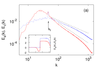
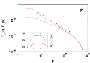
Figure 15: (a) Power spectra of active (red) and passive (blue) scalar variances $E_{a}(k)=\pi k|\hat{a}({\bm{k}},t)|^{2}$ and $E_{c}(k)=\pi k|\hat{c}({\bm{k}},t)|^{2}$ for run 1, the inset shows the active, and passive energy fluxes $\Pi_{a,c}(k)$. The dashed lines corresponds to the best fitted spectral slopes $E_{a}(k)\sim k^{-1.8\pm 0.1}$ and $E_{c}(k)\sim k^{-1.15\pm 0.05}$. Note that the fitted slope for $E_{a}(k)$ is better recovered at higher wavenumbers, close to the energy peak a steeper ($\sim k^{-2\pm 0.1}$) is observed. (b) The same but for run 3. The left inset shows the scalar fluxes. The dashed lines indicates the spectral slopes $E_{a}(k)\sim k^{-1.8\pm 0.1}$ and $E_{c}(k)\sim k^{-1.17\pm 0.05}$. Here the scaling range is wider than in run 1. For both runs active and passive spectra have been shifted for visualization purposes. In the other runs we observe the same qualitative and quantitative features, within the error bars. In particular, run 1 and run 2 give almost indistinguishable spectral slopes, meaning that the large scale energy sink does not enter too much into the inertial range, as expected since the velocity field is rough at small scales. Run 5 produced spectral slopes indistinguishable from those of runs 3 and 4. However, it should be noted that run 1 and run 2 display a steeper spectra close to the forcing wave numbers, this feature is absent in the other runs and may be due to finite size effects, see text and also Fig. 17.

Two observations are in order:

$\bullet$ The scalar spectra $E_{a}(k)$ is steeper than the dimensionally expected $k^{-5/3}$. The slope does not seem to depend on the injection mechanism.

$\bullet$ The active and passive scalars, both performing a direct cascade, are different already at the level of the spectral slopes. In particular, $c$ is much rougher than $a$.

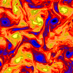
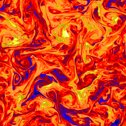
Figure 16: Snapshots of the active (left) and passive (right) scalar (at $512^{2}$ resolution). Note the presence of coherent structures in the active field, which are slow evolving. The passive field displays filamental like features indicating that it is more rough than the active one.

The differences between $a$ and $c$ are evident also from Fig. 16, where two simultaneous snapshots of the fields are displayed. A direct inspection of the fields confirms that $c$ is more rough than $a$, and resembles a passive scalar in a smooth flow. Moreover, in $a$ we observe the presence of large coherent structures at the scale of the forcing. These are actually long-lived, slowly-evolving structures that strongly impair the convergence of the statistics for high-order structure functions. In the following we thus limit ourselves to a comparison of the low-order statistics of $a$ and $c$. That is however sufficient to appreciate the differences beween active and passive scalar statistics.

Figure 17: (a) Second order structure function for the active (empty boxes) and the passive (full circles) scalar in run 2. The straight line shows the scaling $\sim r^{1}$ for the $S^{a}_{2}(r)$ (the same exponent is observed in run 1). The passive scalar does not display a neat scaling behavior. In the inset we show the correlation function for the passive scalar, ${\cal C}^{c}_{2}(r)$, in log-lin scale, (see text). (b) The same but for run 3. Here the straight dashed line indicates the slope $r^{0.8}$. $S^{a}_{2}(r)$ in run 5 has a slope $\sim r^{0.84}$, compatible with the ones observed in runs 3 and 4 within statistical errors.

The deviation from the dimensional expectation for the spectral slope of the active field was already observed in previous numerical studies [9], and it is possibly due to intermittency in the active scalar and velocity statistics. Indeed, the rescaled pdfs of the increments do not collapse (not shown). Concerning the universality of anomalous exponents with respect to the forcing statistics, we observe that the spectral slopes do not depend sensitively on the forcing statistics. However, the forcing (B) (see table 1) induces a steeper spectrum close to the forcing scale, while a universal slope is apparently recovered at large wavenumbers. (Fig. 15a). The scaling of $S^{a}_{2}(r)$ seems to be more sensitive to the forcing (see Fig. 17). These discrepancies may be due to finite size effects which are more severe for forcing (B) which is characterized by a slower decay of the spatial correlations. Unfortunately, it is difficult to extract reliable information on the high-order statistics. Indeed the presence of slowly evolving coherent structures induces a poorly converging statistics for high-order structure functions. Therefore, we cannot rule out the possibility of a dependence of active scalar exponents on forcing statistics.

A result that emerges beyond any doubt is that active and passive scalars behave differently, as shown in Figs. 15, 16 and 17. This is confirmed by the differences in the pdfs of $\delta_{r}a$ and $\delta_{r}c$ at various scales within the inertial range (Fig. 18). The single-point pdfs of $a$ and $c$ are different as well (not shown).

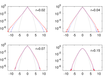
Figure 18: Pdf of active (red) and passive (blue) scalar differences normalized by their respective standard deviations for four different scales within the inertial range. The dotted lines are Gaussian pdfs drawn for comparison. Data refer to run 3, the other runs show similar results.

It is worth noticing that the behavior of the passive scalar deviates from naïve expectations. We observe $E_{c}(k)\sim k^{-1.15}$ whereas a dimensional argument based on the observed velocity spectrum ($E_{v}(k)\equiv E_{a}(k)\sim k^{-1.8}$) and on the Yaglom relation [4] ($\langle\delta_{r}v\,(\delta_{r}c)^{2}\rangle\sim r$) would give $E_{a}(k)\sim k^{-1.6}$. The violation of the dimensional prediction is even more striking looking at $S^{c}_{2}(r)$ in Fig. 17. This feature is reminiscent of some experimental investigations of passive scalars in turbulent flows, see e.g. Refs. [62, 63] and references therein, where shallow scalar spectra are observed for the scalar even at those scales where the velocity field displays a K41 spectrum. It is likely that the presence of coherent structures (see Fig. 16) leads to persistent regions where the velocity field has a smooth (shear-like) behavior. This suggest a two-fluid picture: a slowly evolving shear-like flow, with superimposed faster turbulent fluctuations. Under those conditions, one may expect that the particle pairs separate faster than expected, leading to shallower passive scalar spectra [64].

In conclusion, even though both passive and active scalar perform a direct cascade, their statistical properties are definitely different.

6.3 Scaling and geometry

Let us now compare the two scalars field by investigating the three-point correlation functions of the active field, ${\cal C}^{a}_{3}({\bm{x}}_{1},{\bm{x}}_{2},{\bm{x}}_{3})=\langle a({\bm{x}}_{1},t)a({\bm{x}}_{2},t)a({\bm{x}}_{3},t)\rangle$, and of the passive one, ${\cal C}^{c}_{3}({\bm{x}}_{1},{\bm{x}}_{2},{\bm{x}}_{3})=\langle c({\bm{x}}_{1},t)c({\bm{x}}_{3},t)c({\bm{x}}_{3},t)\rangle$. This allows to compare the scaling properties of the correlation function by measuring the dependence on the global size of the triangle identified by the three points, $R^{2}=\sum_{i<j}x_{ij}^{2}$ (being $x_{ij}=|{\bm{x}}_{i}-{\bm{x}}_{j}|$). We will also investigate the geometrical dependence of $C_{3}$.

It has to be noted that for $\delta$-correlated Gaussian forcings as (23) and (27), ${\cal C}_{3}^{a}$ and ${\cal C}_{3}^{c}$ are identically zero. Therefore we need a different forcing statistics in order to study three-point correlations. A possibility is to break the rotational symmetry of the system by an anisotropic forcing, e.g., a mean gradient (24) as in [28]. However, that choice leads inevitably to $a=c$: the equations are identical for $a$ and $c$ so that the difference field $a-c$ will decay out. We then choose to force the system as follows. The two inputs $f_{a}$ and $f_{c}$ are

$$f_{a,c}({\bm{x}},t)=g_{a,c}^{2}({\bm{x}},t)-\int{\rm d}{\bm{y}}g_{a,c}^{2}({\bm{y}},t)$$ (51)

where $g_{a,c}$ is a homogeneous, isotropic and Gaussian random field with correlation

$$\langle g_{i}({\bm{x}},t)g_{j}({\bm{x}}^{\prime},t^{\prime})\rangle=\delta_{i,j}{\cal G}(|{\bm{x}}-{\bm{x}}^{\prime}|/\ell_{f})e^{-{|t-t^{\prime}|\over\tau_{f}}}\,,$$ (52)

where $i,j=a,c$, $\ell_{f}$ is the forcing scale, $\tau_{f}$ the forcing correlation time and ${\cal G}(r)\propto G_{0}\exp(-r^{2}/2)$. The time correlation is imposed by performing an independent Ornstein-Uhlenbeck process at each Fourier mode, i.e. integrating the stochastic differential equation $d\hat{g_{i}}({\bm{k}},t)=-1/\tau_{f}\hat{g_{i}}({\bm{k}},t)dt+\sqrt{2G_{0}dt/\tau_{f}}dw_{i}({\bm{k}},t)$ (where $dw_{i}$ are zero mean Gaussian variables with $\langle dw_{i}({\bm{k}},t)dw_{j}({\bm{k}}^{\prime},t^{\prime})\rangle=\delta_{i,j}\delta(t-t^{\prime})\delta({\bm{k}}-{\bm{k}}^{\prime})$). If $\tau_{f}\ll{\cal T}_{\ell_{f}}$ by the central limit theorem a Gaussian statistics is recovered. Therefore, we fixed $\tau_{f}\sim O({\cal T}_{\ell_{f}})$ in our DNS. The advantages of this choice are that it preserves the isotropy and gives analytical control on the forcing correlation functions.

Let us now see how the triangle identified by the three points, $\underline{\bm{x}}=({\bm{x}}_{1},{\bm{x}}_{2},{\bm{x}}_{3})$ can be parameterized. In two dimensions we need $3d=6$ variables to define a triangle. Since the correlation functions should possess all the statistical symmetries of the system the number of degrees of freedom is reduced. In particular, translational invariance ensures no dependence on the position of the center of mass of the triangle, $({\bm{x}}_{1}+{\bm{x}}_{2}+{\bm{x}}_{3})/3$. The correlation function is thus a function of the separation vectors among the $3$ points, i.e. ${\cal C}_{3}^{a,c}(\underline{\bm{x}})={\cal C}_{3}^{a,c}({\bm{x}}_{12},{\bm{x}}_{23},{\bm{x}}_{31})$. Additionally, isotropy implies that a rigid rotation of the triangle has no effect on the value of $C_{3}$, so that three variables suffice: the global size of the triangle $R$, and two parameters that define its shape. In terms of the Euler parametrization [65, 66, 67], upon defining ${\bm{\rho}}_{1}=({\bm{x}}_{1}-{\bm{x}}_{2})/\sqrt{2}$ and ${\bm{\rho}}_{2}=({\bm{x}}_{1}+{\bm{x}}_{2}-2{\bm{x}}_{3})/\sqrt{6}$, the shape of the triangle is given in terms of the two variables:

$$w={2{\bm{\rho}}_{1}\times{\bm{\rho}}_{2}\over R^{2}}\,\qquad\chi={1\over 2}\tan^{-1}\left[{2\,{\bm{\rho}}_{1}\cdot{\bm{\rho}}_{2}\over\rho_{1}^{2}-\rho_{2}^{2}}\right]\,,$$ (53)

where $|w|$ is the ratio of the area of the triangle divided by the area of the equilateral triangle having the same size, $R^{2}=\rho_{1}^{2}+\rho_{2}^{2}$. $\chi$ has not a simple geometrical interpretation. Some shapes corresponding to a few $(w,\chi)$ are shown in Fig. 19.

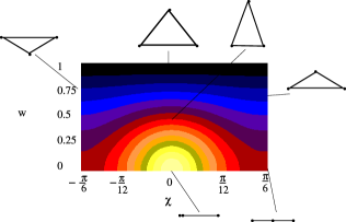
Figure 19: Contour plots in the $\chi-w$ plane of the three-point shape function, $\Phi$, for passive (left) and active (right) scalar.

The three-point correlation function can be decomposed as [31, 27]

$${\cal C}^{a,c}_{3}(\underline{\bm{x}})={\cal R}\{{\cal C}^{a,c}_{3}(\underline{\bm{x}})\}+{\cal I}\{{\cal C}^{a,c}_{3}(\underline{\bm{x}})\}\,,$$ (54)

where ${\cal R},{\cal I}$ are the reducible and irreducible components, respectively. This means that ${\cal C}_{3}$ can be expressed as the sum of a part that depends on three points (hereafter denoted as $C_{3}$) and a part that depends on two points (hereafter denoted $C_{2}$), i.e. ${\cal C}_{3}({\bm{x}}_{1},{\bm{x}}_{2},{\bm{x}}_{3})=C_{3}({\bm{x}}_{1},{\bm{x}}_{2},{\bm{x}}_{3})+C_{2}({\bm{x}}_{1},{\bm{x}}_{2})+C_{2}({\bm{x}}_{2},{\bm{x}}_{3})+C_{2}({\bm{x}}_{3},{\bm{x}}_{1})$. The reducible, ${\cal R}\{{\cal C}_{3}\}=C_{2}({\bm{x}}_{1},{\bm{x}}_{2})+C_{2}({\bm{x}}_{2},{\bm{x}}_{3})+C_{2}({\bm{x}}_{3},{\bm{x}}_{1})$ and irriducible part ${\cal I}\{{\cal C}_{3}\}=C_{3}({\bm{x}}_{1},{\bm{x}}_{2},{\bm{x}}_{3})$ are in general characterized by different scaling properties as a function of the triangle size $R$, and different geometrical (shape) dependencies [68, 28].

In terms of the variables $R,w$ and $\chi$, the reducible and irreducible components take the following form

$${\cal R}\{{\cal C}^{a,c}_{3}(\underline{\bm{x}})\} = h_{a,c}^{\cal R}(R)\Phi^{{\cal R}}_{a,c}(\chi,w)\,,$$

$${\cal I}\{{\cal C}^{a,c}_{3}(\underline{\bm{x}})\} = h_{a,c}^{\cal I}(R)\Phi^{{\cal I}}_{a,c}(\chi,w)\,,$$ (55)

where the function $h(R)$ is expected to have a scaling dependence in the inertial range.

For the passive scalar, the scaling behavior of the reducible part, $h^{\cal R}_{c}(R)$, is dominated by the dimensional scaling imposed by the balance with the forcing, while the scaling of the irreducible part, $h^{\cal R}_{c}(R)$, is given by the zero modes [31]. With a finite-correlated pumping the forcing statistics may in principle contribute to the irreducible part [27]; however in our case these hypothetical contributions seem small, if not absent. For the active scalar it is not possible to make any a priori argument to predict the scaling behavior of the reducible and irreducible part. As far as the geometrical dependence is concerned, $\Phi^{\cal R,I}_{c}$ and $\Phi^{\cal R,I}_{a}$, it is very difficult to separate the two contributions. In our case, in agreement with the results obtained for the Kraichanan model [68], the reducible part turns out to be the leading contribution, so that we only present the shape dependence of the full correlation functions which basically coincides with the reducible one. Hereafter we will then use $\Phi_{a,c}$ dropping the indices which distinguish the two contributions.

Figure 20: (a) $h^{\cal R}(R)$ vs $R$ for the active ($\circ$) and passive ($\Box$) scalar. The dashed lines are the second order structure functions, $S^{a,c}_{2}$, multiplied by a factor to allow for a comparison. The solid line gives the fitted slope, $R^{1.23\pm 0.05}$, for $h^{\cal R}_{a}(R)$. The slope of $S^{a}_{2}$ is $\approx r^{.84\pm 0.05}$ and is compatible with those obtained with the forcing (G), see Fig. 17). The passive curves have been shifted for visualization purposes. (b) $h^{\cal I}_{a,c}(R)$ vs $R$ for the active ($\circ$) and passive ($\Box$) scalar. For $c$ the scaling $R^{1.7\pm 0.2}$ (solid line) is measured. The signal for the active scalar is very low and no scaling behavior can be detected. The statistics has been computed averaging over about $65$ frames separated by half eddy turnover time.

Let us start by studying the shape dependence of the correlation function for the active, $\Phi_{a}(\chi,w)$, and passive scalars, $\Phi_{c}(\chi,w)$. Exploiting the invariance under arbitrary permutations of the three veritices of the triangle we can reduce the configuration space to $\chi\in[-\pi/6:\pi/6]$, and $w\in[0:1]$ going from degenerate (collinear points) to equilateral triangles. The function $\Phi(\chi,w)$ is antiperiodic in $\chi$ with period $\pi/3$ [65, 66, 67]. In Fig. 19 the functions $\Phi_{c}$ and $\Phi_{c}$ are shown. They have been measured for a fixed size $R$ within the inertial range. The two functions display similar qualitative features: the intensity grows going from equilateral to collinear triangles, and the maximum is realized for almost degenerate triangles $(\chi,w)=(0,0)$. $\Phi_{c}$ is invariant for $\chi\to-\chi$, which corresponds to reflection with respect to an axis. This symmetry is a consequence of the equation of motion and the fact that $f_{c}\to f_{c}$ under this symmetry transformation. The active scalar displays a weak breaking of this symmetry, as a consequence of the fact that it is a pseudoscalar while $f_{a}$ is not.

Let us now turn our attention to the scaling behavior. Since the reducible scaling behavior is the leading one it is simply obtained by fixing a certain shape for the triangle (we did for several choices of $(\chi,w)$) and varying its size. The results are shown in in Fig. 20a. The observation is that $h^{\cal R}_{a}(R)$ and $h^{\cal R}_{c}(R)$ are different. Moreover, while $h^{\cal R}_{c}(R)$ is practically parallel to $S^{c}_{2}(R)$, for the active scalar we observe that $h^{\cal R}_{a}(R)$ is not scaling as $S^{a}_{2}(R)$.

The measure of the subleading, irreducible part is more involved, and we proceed as follows. We fix a reference triangle shape $(\chi,w)$ and set the origin in the center of mass of the triangle. Now ${\bm{x}}_{i}$ indicates the position of the vertex $i$ of the triangle. We define $\hat{d}_{1}=\hat{d}_{1}(\lambda)$ ($\lambda\geq 1$) as the dilation operator which transforms the triangle $({\bm{x}}_{1},{\bm{x}}_{2},{\bm{x}}_{3})$ in $(\lambda{\bm{x}}_{1},{\bm{x}}_{2},{\bm{x}}_{3})$. Analogous definitions hold for the other vertices. Obviously $\hat{d}_{i}(1)\equiv\hat{I}$ is the identity. We then consider the composite operator $\hat{\cal D}(\lambda)=\hat{d}_{1}\hat{d}_{2}\hat{d}_{3}-\hat{d}_{1}\hat{d}_{2}-\hat{d}_{2}\hat{d}_{3}-\hat{d}_{3}\hat{d}_{1}+\hat{d}_{1}+\hat{d}_{2}+\hat{d}_{3}-\hat{I}$. By direct substitution it is easily seen that in $\hat{\cal D}(\lambda){\cal C}_{3}({\bm{x}}_{1},{\bm{x}}_{2},{\bm{x}}_{3})$ all the reducible terms are cancelled, and only a linear superposition of terms involving the irreducible parts survives Therefore, the average of $\hat{\cal D}(\lambda)c({\bm{x}}_{1})c({\bm{x}}_{2})c({\bm{x}}_{3})$ for triangles of different sizes $R$ but of fixed shape $(\chi,w)$ will give the scaling of the irreducible part of the three-point function. (55). A similar procedure has been done for $a$. We used as reference configuration a collinear triangle with two degenerate vertices, i.e. $(\chi,w)=(0,0)$. This choice reduces the number of cancellations. Additionally, this configuration corresponds to the region of stronger gradients in the function $\Phi$ (see Fig. 19), yielding a higher signal to noise ratio. By varying $\lambda$ we tested the robustness of the measured scaling.

In Fig. 20 we present the results on the scale dependence of $h^{\cal I}_{c}(R)$ and $h^{\cal I}_{a}(R)$. Clearly $h^{\cal I}_{a}(R)$ has too low a signal to identify any scaling behavior, while the passive scalar scales fairly well and we measured $h^{\cal I}_{c}(R)\sim R^{1.7}$, confirming that the irreducible part is subleading.

A couple of final remarks are in order. First, the fact that $h^{\cal R}_{a}(R)$ does not scale as $S^{a}_{2}(R)$ is the signature of the correlations between $f_{a}$ and the particle propagator. Indeed, for the passive scalar $h^{\cal R}_{c}(R)\propto S^{c}_{2}(R)$ is a straightforward consequence of the independence of ${\bm{v}}$ and $f_{c}$. Second, $h^{\cal R}_{a}(R)$ scales differently from $h^{\cal I}_{c}(R)$: this rules out the possibility of establishing simple relationships between active and passive scalar statistics (see [15] for a related discussion).

7 Conclusions and perspectives

In summary, we have investigated the statistics of active and passive scalars transported by the same turbulent flow. We put the focus on the issue of universality and scaling. In this respect the passive scalar problem is essentially understood. Conversely, the active case is by far and away a challenging open problem. The basic property that make passive scalar turbulence substantially simpler is the absence of statistical correlations between scalar forcing and carrier flow. On the contrary, the hallmark of active scalars is the functional dependence of velocity on the scalar field and thus on active scalar pumping. Yet, when correlations are sufficiently weak, the active scalar behaves similarly to the passive one: this is the case of two-dimensional thermal convection and Ekman turbulence. However, this appears to be a nongeneric situation, and the equivalence between passive and active scalar is rooted in special properties of those systems. Indeed, different systems as two-dimensional magnetohydrodynamics or surface quasi-geostrophic turbulence are characterized by a marked difference between passive and active scalar statistics. This poses the problem of universality in active scalar turbulence: if the forcing is capable of influencing the velocity dynamics, how can scaling exponents be universal with respect to the details of the injection mechanism ? So far, a satisfactory answer is missing. As of today, numerical experiments favor the hypothesis that universality is not lost in a number of active scalars, but further investigation is needed to elucidate this fundamental issue.

References

References

- [1] Pasquill F and Smith F B 1983 Atmospheric Diffusion (Ellis Horwood, Chichester)
- [2] Williams F A 1985 Combustion Theory (Benjamin-Cummings, Menlo Park)
- [3] Zel’dovich Ya B , Ruzmaikin A and Sokoloff D 1983 Magnetic Fields in Astrophysics (Gordon and Breach, New York)
- [4] Monin A and Yaglom A 1975 Statistical Fluid Mechanics (MIT Press, Cambridge, Mass.)
- [5] Siggia E D 1994 Ann. Rev. Fluid Mech. 26, 137
- [6] Biskamp D 1993 Nonlinear Magnetohydrodynamics, (Cambridge University Press, Cambridge UK)
- [7] Salmon R 1998 Geophysical Fluid Dynamics, (Oxford University Press, New York, USA)
- [8] Rhines P B 1979 Ann. Rev. Fluid Mech. 11, 401
-
[9]
Pierrehumbert R T, Held I M and Swanson K L 1994
Chaos, Sol. and Fract. 4, 1111
Held I M, Pierrehumbert R T, Garner S T and Swanson K L 1995 J. Fluid Mech 282, 1 - [10] Constantin P 1998 J. Stat. Phys. 90, 571
- [11] Celani A, Matsumoto T, Mazzino A and Vergassola M 2002 Phys. Rev. Lett. 88, 054503
- [12] Boffetta G, Celani A, Musacchio A and Vergassola M 2002 Phys. Rev. E 66, 026304
- [13] Celani A, Cencini M, Mazzino A and Vergassola M 2002 “Active versus Passive Scalar Turbulence”, Phys. Rev. Lett. 89, 234502
- [14] Ching E S C, Cohen Y, Gilbert T and Procaccia I 2002 Europhys. Lett. 60, 369
- [15] Ching E S C, Cohen Y, Gilbert T and Procaccia I 2003 Phys. Rev. E 67, 016304
- [16] Nam K, Antonsen T M, Guzdar P N and Ott E 1999 Phys. Rev. Lett. 83, 3426
- [17] Nam K, Ott E, Antonsen T M and Guzdar P N 2000 Phys. Rev. Lett. 84, 5134
- [18] Frisch U 1995 Turbulence: The Legacy of A. N. Kolmogorov (Cambridge: Cambridge University Press)
- [19] Warhaft Z 2000 Annu. Rev. Fluid Mech. 32, 203
- [20] Moisy F, Willaime H, Andersen J S and Tabeling P 2001 Phys. Rev. Lett. 86, 4827
-
[21]
Celani A, Lanotte A, Mazzino A and Vergassola M 2000
Phys. Rev. Lett. 84, 2385
Celani A, Lanotte A, Mazzino A and Vergassola M 2001 Phys. Fluids 13, 1768 - [22] Kraichnan R H 1968 Phys. Fluids 11, 945
- [23] Kraichnan R H 1994 Phys. Rev. Lett. 72, 1016
- [24] Gawȩdzki K and Kupiainen A 1995 Phys. Rev. Lett. 75, 3834
- [25] Chertkov M, Falkovich G, Kolokolov I and Lebedev V 1995 Phys. Rev. E 52, 4924
- [26] Shraiman B I and Siggia E D 1995 C. R. Acad. Sci. Paris, série II 321, 279
- [27] Falkovich G, Gawȩdzki K and Vergassola M 2001 Rev. Mod. Phys. 73, 913
- [28] Celani A and Vergassola M 2001 Phys. Rev. Lett. 86, 424
- [29] Frisch U, Mazzino A, Noullez A and Vergassola M 1999 Phys. Fluids 11, 2178
- [30] Risken H 1998 The Fokker Planck Equation (Springer Verlag, Berlin)
- [31] Bernard D, Gawȩdzki K and Kupiainen A 1998 J. Stat. Phys. 90, 519
- [32] Arad I, Biferale L, Celani A, Procaccia I and Vergassola M 2001 Phys. Rev. Lett. 87, 164502
- [33] Chertkov M, Kolokolov I and Vergassola M, 197 Phys. Rev. E 56, 5483
- [34] Gawȩdzki K and Vergassola M 2000 Physica D 138, 63
- [35] Yakhot V 1997 Phys. Rev. E 55, 329
- [36] Bizon C, Werne J, Predtechensky A A, Julien K, McCormick W D, Swift J B and Swinney H L 1997 Chaos 7, 1
- [37] Rivera M and Wu X L 2000 Phys. Rev. Lett. 85, 976
- [38] Celani A, Mazzino A and Vergassola M 2001 Phys. Fluids 13, 2133
- [39] Zhou S-Q and Xia K-Q 2002 Phys. Rev. Lett. 89, 184502
- [40] Antonelli M, Mazzino A and Rizza U 2003 J. Atmos. Sci. 60, 215
- [41] Paret J and Tabeling P 1998 Phys. Fluids 10, 3126
- [42] Boffetta G, Celani A and Vergassola M 2000 Phys. Rev. E 61, R29
- [43] Pouquet A 1978 J. Fluid. Mech 88, 1
- [44] Celani A, Cencini M and Noullez A 2004 “Going forth and back in time: a fast and parsimonious algorithm for mixed initial/final-value problems”, Physica D to appear Preprint physics/0305058
- [45] Biskamp D and Bremer U 1994 Phys. Rev. Lett. 72, 3819
- [46] To obtain the r.h.s. of (31) consider the expression , insert , i.e. Eq. (4) evaluated at time , and exploit the symmetry under exchange of and to switch from a time-ordered form to a time-symmetric one to get rid of the factor two.
- [47] Sridhar S and Goldreich P 1994 Astroph. J. 432, 612
- [48] Verma M K, Roberts D A, Goldstein M L, Ghosh S and Stribling W T 1996 J. Geophys. Res. 101, 21619
- [49] Politano H, Pouquet A and Carbone V 1998 Europhys. Lett. 43, 516
- [50] Biskamp D and Schwarz E 2001 Phys. Plasmas 8, 3282
- [51] Kraichnan R H 1967 Phys. Fluids 10, 1417
- [52] G. K. Batchelor G K 1969 Phys. Fluids. Suppl. II 12, 233
- [53] Paret J, Jullien M C and Tabeling P 1999 Phys. Rev. Lett. 83, 3418
- [54] Chertkov M 1999 Phys. Fluids 11, 2257
- [55] Jullien M C, Castiglione P and Tabeling P 2000 Phys. Rev. Lett. 85, 3636
- [56] Bernard D 2000 Europhys. Lett. 50, 333
- [57] Crisanti A, Paladin G and Vulpiani A 1993 Products of Random Matrices (Springer Verlag, Berlin)
- [58] Ellis R S 1985 Entropy, Large Deviations, and Statistical Mechanics (Springer-Verlag, New York)
- [59] Constantin P 2002 Phys. Rev. Lett. 89, 184501
- [60] Constantin P 1995 Physica D 86, 212
- [61] Majda A and Tabak E 1996 Physica D 98, 515
- [62] Villermaux E, Innocenti C and Duplat J 2001 Phys. Fluids 13, 284
- [63] Villermaux E and Innocenti C 1999 J. Fluid Mech. 393, 123
- [64] Celani A, Cencini M, Vergassola M, Vincenzi D and Villermaux E 2004 in preparation
- [65] Shraiman B I and Siggia E D 1998 Phys. Rev. E 57, 2965
- [66] Pumir A 1998 Phys. Rev. E 57, 2914
- [67] Castiglione P and Pumir A 2001 Phys. Rev. E 64, 056303
- [68] Gat O, L’vov V S and Procaccia I 1997 Phys. Rev. E 56, 406