Effect of the introduction of impurities on the stability properties of multibreathers at low coupling

Abstract

Using a theorem dubbed the Multibreather Stabiliy Theorem [Physica D 180 (2003) 235-255] we have obtained the stability properties of multibreathers in systems of coupled oscillators with on-site potentials, with an inhomogeneity. Analytical results are obtained for 2-site, 3-site breathers, multibreathers, phonobreathers and dark breathers. The inhomogeneity is considered both at the on-site potential and at the coupling terms. All the results have been checked numerically with excellent agreement. The main conclusion is that the introduction of a impurity does not alter the stability properties.

1 Introduction

Discrete breathers (DBs) are periodic, localized solutions that appear in discrete lattices of nonlinear oscillators. For Klein-Gordon lattices, i.e, lattices with an on-site potential, the conditions for their existence at low coupling are very weak. They are based on properties of the lattice at the anti continuous limit, that is, the same lattice with zero coupling and, then, with the oscillators isolated. These conditions can be expressed in simple words as: a) For a given frequency $\omega_{\mathrm{b}}$ the isolated oscillator is truly nonlinear ($\mathrm{d}E/\mathrm{d}\omega_{\mathrm{b}}\neq 0$, with $E$ the energy of the isolated oscillator). b) The breather does not resonate with the phonons ($n\,\omega_{\mathrm{b}}\neq\omega_{\mathrm{o}}$, with $n$ any positive integer and $\omega_{\mathrm{o}}$ the frequency of the isolated oscillators [1]. The stability of one–site breathers has been proven in [2, 3, 4], whereas the stability of two-sites breathers was proven in Ref. [5]. Recently, some of the authors developed the Multibreathers Stability Theorem (MST) [6], which provides with a method for obtaining the stability properties of any multibreather at low-coupling and applied it to homogeneous lattices. Although the MST applies to any Klein-Gordon lattice, it depends on the analytical or numerical calculation of some magnitudes $J_{nm}$ : This calculation becomes less simple and the number of magnitudes larger as the system becomes more complicated, involving, for example, different linear frequencies or initial phases for the oscillators.

In this paper we address the application of the MST to Klein-Gordon lattices with an impurity. This impurity can be modelled at the on-site potential or at the coupling. The implementation of it at the masses is equivalent to at the on-site potential. The necessary magnitudes are calculated and the MST applied to 2-sites and 3-site breathers, multibreathers, phonobreathers and dark breathers. The theoretical results are also checked numerically to confirm the validity of the calculations with excellent results.

The paper is organized in the following form: first we describe the details of the model; second we recall the Multibreathers Stability Theorem, and give some details of its application to the case of a lattice with an impurity. Subsequent sections particularize it for two and three–sites breathers, phonobreathers, multibreathers and dark breathers. Details of analytical calculations are relegated to the first appendix. In the second appendix, a conjecture made in Ref. [6] is proven. It is that the only multibreathers that can be stable are the ones with all the oscillator in phase or out of phase.

2 The model

In this paper, we consider Klein–Gordon chains with linear nearest-neighbours coupling whose dynamical equations are of the form:

$$\ddot{u}_{n}\,+\,V^{\prime}(u_{n})\,+\,\varepsilon\,\sum_{m=1}^{N}\,C_{nm}u_{n}\,=\,0\,\quad n=1,\dots,N$$ (1)

where the variables $u_{n}$ are the displacements with respect to the equilibrium positions, $V(u_{n})$ is the on–site potential, $N$ is the number of oscillators, $C$ is a coupling matrix which includes the boundary conditions, and $\varepsilon$ is the coupling parameter.

The impurity can be introduced in the system through an inhomogeneity at the on–site potential or the coupling matrix, in a similar fashion as it was done in [7].

The linear frequencies of the isolated oscillators are $\omega_{\mathrm{n}}=(V_{n}^{\prime\prime}(0))^{1/2}$. If the inhomogeneity is implemented at the potential of the $n_{0}$-th particle, we denote $V_{0}=V_{n}$ and $\omega_{\mathrm{o}}=\omega_{\mathrm{n}}=(V_{0}^{\prime\prime}(0))^{1/2}$ $\forall n\neq n_{0}$. We can write $\omega_{\mathrm{n0}}^{2}=(1+\alpha\delta_{n,n_{0}})\,\omega_{\mathrm{o}}$, where the inhomogeneity parameter $\alpha$ takes values in $(-1,\infty)$, $\alpha=0$ corresponding to the homogeneous case.

For a system with nearest-neighbour interaction, the dynamical equations Eq. (1) can be written [7]:

$$\ddot{u}_{n}\,+\,V^{\prime}(u_{n})\,+\,\varepsilon\,[\,k_{n-1,n}\,(u_{n}-u_{n-1})+k_{n,n+1}\,(u_{n}-u_{n+1})\,]=\,0\,.$$ (2)

If the system is homogeneous $k_{n,m}=1$, $\forall n,m$, except at $m=1$ or $n=N$ for a system with $N$ oscillators. With periodic boundary conditions, the index $n$ is cyclical so as $0\sim N$ and $N+1\sim 1$ and $k_{0,1}=k_{N,N+1}=1$. With free ends, $k_{0,1}=k_{N,N+1}=0$. With fixed ends, two extra oscillators have $u_{0}=u_{N+1}=0$ and $k_{0,1}=k_{N,N+1}=1$.

Therefore, the coupling matrix, $C^{0}$ for a finite system with $N$ oscillators with fixed ends (at the oscillators $n=0$ and $n=N+1$), has elements:

$$C^{0}_{nm}=\left\{\begin{array}[]{ll}2&\textrm{if }n=m\\ -1&\textrm{if }|n-m|=1\\ 0&\textrm{otherwise}.\end{array}\right.$$ (3)

With free ends, $C_{1\,1}=C_{N\,N}=1$, and with periodic boundary conditions, $C_{1\,N}=C_{N\,1}=-1$.

We model the impurity at a site $n_{0}$ distinct from the lattice boundaries, by changing the constants $k_{{n{\small 0}},{n{\small 0}}+1}$ and $k_{{n{\small 0}}-1,{n{\small 0}}}$ to $(1+\beta/2)$, with $\beta$ being a parameter which takes its values in $(-2,\infty)$, so as the homogeneous case is recovered when $\beta=0$. $\beta<0$ means weaker constants than the homogeneous coupling ones and $\beta>0$ the opposite.

Therefore, the coupling matrix $C_{nm}$ becomes:

$$C_{nm}=\left\{\begin{array}[]{ll}(\beta+2)&\textrm{if }n=m=n_{0}\\ -(\beta+2)/2&\textrm{if }|n-m|=1\textrm{ and }n=n_{0}\textrm{ or }m=n_{0}\\ (\beta+4)/2&\textrm{if }n=m=n_{0}\pm 1\\ C^{0}_{nm}&\textrm{otherwise},\end{array}\right.$$ (4)

3 Stability theorem

In this section we recall some results of the multibreather stability theorems established in Ref. [6]. For more details about this theory, the reader is referred to that reference.

The stability of a multibreather at low coupling can be established through three different parameters: the sign of the coupling constant $\varepsilon$, the softness/hardness of the on-site potential and the sign of the eigenvalues $\{\lambda_{i}\}$ of the perturbation matrix $Q$, to be described below. Considering a positive coupling constant, the multibreather is stable for a soft potential if all the eigenvalues of $Q$ are non-negative ($Q$ is positive semi-definite); if the potential is soft, the multibreather is stable if all the eigenvalues $\{\lambda_{i}\}$ are negative except for a zero one ($Q$ is negative semi-definite). If the coupling constant is negative, the results are reversed. Furthermore, if $Q$ is non-definite (i.e. there are some positive and some negative eigenvalues), the multibreather is unstable independently on the sign of $\varepsilon$ and the softness/hardness of the potential.

We can summarize the stability properties in the following way. Let $S=1$ mean stability and $S=-1$ instability, $H=1$ correspond to a hard on-site potential, and $H=-1$ to a soft one, and define the $\mathrm{sign}(Q)=1$ if all the eigenvalues of $Q$ but a zero one are positive and $\mathrm{sign}(Q)=-1$ if they are negative except for the zero one, other cases being indefinite. Then, $S=-H\times\mathrm{sign}(Q)\times\mathrm{sign}(\varepsilon)$.

It is also important to take into account that there is always a zero eigenvalue due to a global phase mode. If there were more than one zero eigenvalue, the stability theorem can only predict the instability in the case that there existed eigenvalues of different sign, but not the stability, as the 0–eigenvalue is degenerate.

The perturbation matrix $Q$ is obtained in the following way: suppose that at the anticontinuous limit there are $p$ excited oscillators and $N-p$ oscillators at rest. Let us construct the modified coupling matrix $\tilde{C}$ by suppressing in $C$ the rows and columns corresponding to the $N-p$ oscillators at rest, and redefine $C=\tilde{C}$. The dimension of $C$ is $p\times p$, its nondiagonal elements being [6]:

$$Q_{nm}=\frac{{C}_{nm}}{\mu_{n}\,\mu_{m}}\int_{-T/2}^{T/2}\,\dot{u}_{n}\,\dot{u}_{m}\,\mathrm{d}t\,,\quad n\neq m\,\,$$ (5)

with $T=2\,\pi/\omega_{\mathrm{b}}$. The diagonal elements are:

$$Q_{nn}=-\sum_{\forall\,m\neq n}\,\frac{\mu_{m}}{\mu_{n}}\,Q_{nm}\,.$$ (6)

where $u_{n}$ are the solutions of an isolated oscillator submitted to the potential $V(u_{n})$, i.e. the solutions of the equations:

$$\ddot{u}_{n}+V^{\prime}(u_{n})=0,$$ (7)

and $\mu_{n}$ is defined as:

$$\mu_{n}=\sqrt{\int_{-T/2}^{T/2}\,\dot{u}^{2}_{n}\,\mathrm{d}t}$$ (8)

In this paper we limit ourselves to time–reversible solutions, i.e., the excited oscillators at the anticontinuous limit can only have phase $0$ or $\pi$, or, in other words, if $u_{n}(t)$ is a time–reversible solution of Eq. (7), i.e., $u_{n}(t)=u_{n}(-t)$, then $u_{n}(t+T/2)$ is the only possible time–reversible solution apart from $u_{n}(t)$. Therefore, the state of the system at the anticontinuous limit can be described by a code $\sigma=(\sigma_{1},\dots\sigma_{N})$, where $\sigma_{n}=0,+1,-1$ means that the corresponding oscillator is at rest, with phase 0, or with phase $\pi$, respectively, at $t=0$ [2].

Let $J_{nm}$ and $J^{\prime}_{nm}$ be defined as:

$$J_{nm}=\int_{-T/2}^{T/2}\,\dot{u}_{n}(t)\,\dot{u}_{m}(t)\,\mathrm{d}t\,,\quad J^{\prime}_{nm}=\int_{-T/2}^{T/2}\,\dot{u}_{n}(t)\,\dot{u}_{m}(t+T/2)\,\mathrm{d}t\,,\quad$$ (9)

and the parameters $\eta_{nm}$, $\gamma_{nm}$ and $\varphi_{nm}$ as:

$$\eta_{nm}=\frac{\displaystyle J_{nm}}{\displaystyle\sqrt{J_{nn}J_{mm}}}>0,\quad\gamma_{nm}=-\frac{\displaystyle J^{\prime}_{nm}}{\displaystyle\sqrt{J_{nn}J_{mm}}}>0,\quad\varphi_{nm}=\sqrt{\frac{\displaystyle J_{mm}}{\displaystyle J_{nn}}}>0,\quad$$

Then, the matrix elements $Q_{nm}$ can be written as:

$$Q_{nm}=\left\{\begin{array}[]{ll}\eta_{nm}C_{nm}&\textrm{if }\sigma_{n}\sigma_{m}=1\\ -\gamma_{nm}C_{nm}&\textrm{if }\sigma_{n}\sigma_{m}=-1\end{array}\right.$$ (10)

$$Q_{nn}=-\sum_{\forall\,m\neq n}\varphi_{nm}Q_{nm},$$ (11)

where we have taken into account that $\mu_{n}^{2}=J_{nn}$. We have calculated analytically these parameters for several potentials in A, although only the case of the Morse on–site potential leads to relatively simple expressions.

Some properties of the parameters $\eta_{nm}$, $\gamma_{nm}$ and $\varphi_{nm}$ can be easily deduced. In the case of symmetric potentials, $J_{nm}=-J^{\prime}_{nm}$, as $\dot{u}_{n}(t)=-\dot{u}_{n}(t+T/2)$, and, in consequence, $\gamma_{nm}=\eta_{nm}$. Other property is that, for the homogeneous case, $\eta_{nm}=1$, $\varphi_{nm}=1$ and $\gamma_{nm}=\gamma_{0}$, where $\gamma_{0}$ is the symmetry parameter in that case (which is the unity for a symmetric potential).

In order to simplify the notation, as we are considering a single impurity, we define the parameters $\eta\equiv\eta_{nh}$, $\gamma\equiv\gamma_{nh}$, $\varphi\equiv\varphi_{nh}$, where the index $n$ indicates the impurity site and $h$ another one.

4 2-site breathers with an impurity

A 2-site breather is a breather obtained from the anticontinuous limit when two contiguous sites are excited. The boundary conditions are irrelevant as long as the sites are not close to the boundaries. Without loss of generality, let us rename the two indexes so as the impurity is located at $n=1$, and the corresponding oscillator has phase zero ($\sigma_{1}=1$). The other oscillator is located at $n=2$. When dealing with the code $\sigma$ it is enough to consider the codes of these two oscillators, as the other are zero, thus, $\sigma=(\sigma_{1},\sigma_{2})$. Two cases are possible, in–phase oscillators, $\sigma=(1,1)$, and out–of–phase oscillators, $\sigma=(1,-1)$.

4.1 Inhomogeneity at the on-site potential

First of all, we consider the in-phase case. Taking into account Eqs. (3-11) and the notation introduced in Section 3, the matrix $Q$ is given by:

$$Q=\left[\begin{array}[]{cc}\eta\varphi&-\eta\\ -\eta&\eta/\varphi\end{array}\right],$$ (12)

with eigenvalues $\{\lambda_{0},\lambda_{1}\}=\{0,\eta(\varphi+1/\varphi)\}$. Then, $\lambda_{1}>0$.

For the out-of-phase case, the perturbation matrix is:

$$Q=\left[\begin{array}[]{cc}-\gamma\varphi&\gamma\\ \gamma&-\gamma/\varphi\end{array}\right],$$ (13)

with eigenvalues $\{\lambda_{0},\lambda_{1}\}=\{0,-\gamma(\varphi+1/\varphi)\}$. Thus, $\lambda_{1}<0$.

If the system is homogeneous $\{\lambda_{0},\lambda_{1}\}=\{0,2\}$ and $\{\lambda_{0},\lambda_{1}\}=\{0,-2\gamma_{0}\}$ for the in-phase and out-of-phase cases, respectively [6]. In consequence, the sign of $\lambda_{1}$ does not change when an impurity is introduced in the on-site potential, and the stability properties are not altered.

Figs. 1 and 2 show the dependence of $E=\varepsilon\lambda_{1}$ with respect to $\varepsilon$ calculated numerically and analytically (see A). The agreement between both calculations is excellent for fairly large values of the coupling constant.

4.2 Inhomogeneity at the coupling constant

For the $\sigma=(1,1)$ 2–site breather:

$$Q=\frac{\beta+2}{2}\left[\begin{array}[]{cc}1&-1\\ -1&1\end{array}\right]=\frac{\beta+2}{2}Q_{0},$$ (14)

where $Q_{0}$ is the perturbation matrix of the homogeneous chain. Thus, $\lambda_{1}=\beta+2$. The relation $Q=(\beta+2)/2\,Q_{0}$ also holds for the code $\sigma=(1,-1)$, and, in consequence, $\lambda_{1}=-(\beta+2)/2\,\gamma_{0}$ in this case. As $\beta>-2$, the conclusion is that the stability properties are the same as in the homogeneous system.

Fig. 5 compares this result with the numerically obtained.

(a)	(b)
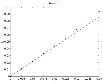
(c)	(d)

Figure 1: Dependence of $E=\varepsilon\lambda_{1}$ with respect to $\varepsilon$ for two different values of $\alpha$. (a,b) correspond to in-phase 2-site breathers and (c,d) to out-of-phase 2-site breathers. All the solutions stand for a Morse potential and $\omega_{\mathrm{b}}=0.8$. Dots represent numerical solutions and lines analytical ones.

(a)	(b)
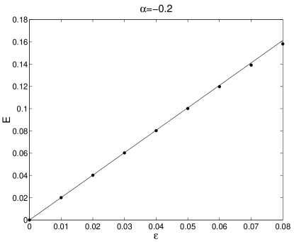
(c)	(d)

Figure 2: Dependence of $E=\varepsilon\lambda_{1}$ with respect to $\varepsilon$ for two different values of $\alpha$. (a,b) correspond to in-phase 2-site breathers and (c,d) to out-of-phase 2-site breathers. All the solutions stand for a hard $\phi^{4}$ potential and $\omega_{\mathrm{b}}=1.3$. Points represent numerical solutions and lines analytical ones.

5 3-site breathers with an impurity

They consist of breathers derived from three contiguous, excited oscillators at the anticontinuous limit. There are seven non–equivalent possibilities, taking into account the position of the impurity and the phases of the oscillators. Let us rename the excited sites as $1,2,3$, suppose that $\sigma_{2}=1$, and denote with boldface the position of the impurity. Then the three-index codes corresponding to the three excited oscillators are (1,1,1), (1,1,1), (-1,1,-1), (-1,1,-1), (1,1,-1), (1,1,-1), (1,1,-1).

5.1 Inhomogeneity at the on-site potential

Let us suppose that the $\sigma\equiv(\sigma_{1},1,\sigma_{3})$. The in-phase breather corresponds to $\sigma_{1}=\sigma_{3}=1$, the out-of-phase to $\sigma_{1}=\sigma_{3}=-1$ and another one to $\sigma_{1}\sigma_{3}=-1$. The following table shows the eigenvalues $\lambda_{1}$ and $\lambda_{2}$ for the different configurations ($\lambda_{0}=0$ always), the impurity site is indicated through a bold font, and, in order to simplify the expressions, we define $\phi=\varphi+1/\varphi$:

Code	$\lambda_{1}$	$\lambda_{2}$
1 1 1	$\eta/\varphi$	$\eta(\varphi+\phi)$
1 1 1	$(2+\eta\phi+\sqrt{4-4\eta\phi+\eta^{2}\phi^{2}})/2$	$(2+\eta\phi+\sqrt{4-4\eta\phi+\eta^{2}\phi^{2}})/2$
-1 1 -1	$-\gamma/\varphi$	$-\gamma(\varphi+\phi)$
-1 1 -1	$-\gamma_{0}-[\gamma\phi+\sqrt{(\gamma\phi+2\gamma_{0})^{2}-4\gamma\gamma_{0}(\varphi+\phi)}]/2$	$-\gamma_{0}-[\gamma\phi-\sqrt{(\gamma\phi+2\gamma_{0})^{2}-4\gamma\gamma_{0}(\varphi+\phi)}]/2$
1 1 -1	$(\eta\phi+\sqrt{\eta^{2}\phi^{2}+4\gamma_{0}\eta(\varphi+\phi)})/2$	$(\eta\phi-\sqrt{\eta^{2}\phi^{2}+4\gamma_{0}\eta(\varphi+\phi)})/2$
1 1 -1	$((\eta-\gamma)\phi+\sqrt{(\eta+\gamma)^{2}\phi^{2}-4\eta\gamma\varphi^{2}})/2$	$((\eta-\gamma)\phi-\sqrt{(\eta+\gamma)^{2}\phi^{2}-4\eta\gamma\varphi^{2}})/2$
1 1 -1	$(-(\gamma\phi-2)+\sqrt{\gamma^{2}\phi^{2}+4+4\gamma\varphi})/2$	$(-(\gamma\phi-2)-\sqrt{\gamma^{2}\phi^{2}+4+4\gamma\varphi})/2$

$\gamma_{0}$ being the symmetry coefficient for the homogeneous case. It can be deduced that $\lambda_{1}>0$ and $\lambda_{2}>0$ for the in-phase solution, $\lambda_{1}<0$ and $\lambda_{2}<0$ for the out-of-phase breather and $\lambda_{1}>0$ and $\lambda_{2}<0$ otherwise. This result coincides with the homogeneous case.

Figs. 3 and 4 show the dependence of $E_{1}=\varepsilon\lambda_{1}$ and $E_{2}=\varepsilon\lambda_{2}$ with respect to $\varepsilon$ calculated numerically and analytically. The agreement between both descriptions is again very good even for fairly large values of the coupling constant.

5.2 Inhomogeneity at the coupling constant

If the impurity is located at $n_{0}=2$, the relation $Q=(\beta+2)/2\,Q_{0}$ is fulfilled again. The only way to obtain a different relation is to suppose the impurity at an edge. The following table summarizes the different cases:

Code	$\lambda_{1}$	$\lambda_{2}$
1 1 1	$1+\beta/2$	$3(1+\beta/2)$
1 1 1	$(\beta+4+\sqrt{\beta^{2}+4})/2$	$(\beta+4-\sqrt{\beta^{2}+4})/2$
-1 1 -1	$-\gamma_{0}(1+\beta/2)$	$-3\gamma_{0}(1+\beta/2)$
-1 1 -1	$-\gamma_{0}(\beta+4+\sqrt{\beta^{2}+4})/2$	$-\gamma_{0}(\beta+4+\sqrt{\beta^{2}+4})/2$
1 1 -1	$1-\gamma_{0}+(\beta+\sqrt{\gamma_{0}^{2}\beta^{2}+2\gamma_{0}(2\gamma_{0}+1)\beta+4(\gamma_{0}^{2}+\gamma_{0}+1)})/2$	$1-\gamma_{0}+(\beta-\sqrt{\gamma_{0}^{2}\beta^{2}+2\gamma_{0}(2\gamma_{0}+1)\beta+4(\gamma_{0}^{2}+\gamma_{0}+1)})/2$
1 1 -1	$(1+\beta/2)(1-\gamma_{0}+\sqrt{\gamma_{0}^{2}+\gamma_{0}+1})$	$(1+\beta/2)(1-\gamma_{0}+\sqrt{\gamma_{0}^{2}+\gamma_{0}+1})$
1 1 -1	$1-\gamma_{0}+(\beta+\sqrt{\gamma_{0}^{2}\beta^{2}+2\gamma_{0}(2\gamma_{0}+1)\beta+4(\gamma_{0}^{2}+\gamma_{0}+1)})/2$	$1-\gamma_{0}+(\beta-\sqrt{\gamma_{0}^{2}\beta^{2}+2\gamma_{0}(2\gamma_{0}+1)\beta+4(\gamma_{0}^{2}+\gamma_{0}+1)})/2$

The signs of the eigenvalues are the same as in the on-site inhomogeneity case. Fig. 5 compares these results with the numerically obtained ones.

(a)	(b)
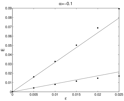
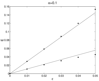
(c)	(d)
(e)	(f)

Figure 3: Dependence of $E=\varepsilon\lambda_{1}$ and $E=\varepsilon\lambda_{2}$ with respect to $\varepsilon$ for two different values of $\alpha$. (a,b) correspond to in-phase 3-site breathers, (c,d) to out-of-phase 3-site breathers with the impurity at the center and (e,f) to the same as before but with the impurity at the edge. All the solutions stand for a Morse potential and $\omega_{\mathrm{b}}=0.8$. Points represent numerical solutions and lines analytical ones.

(a)	(b)
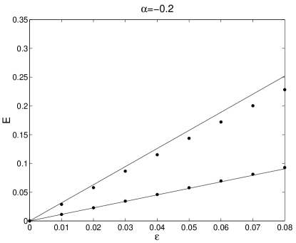
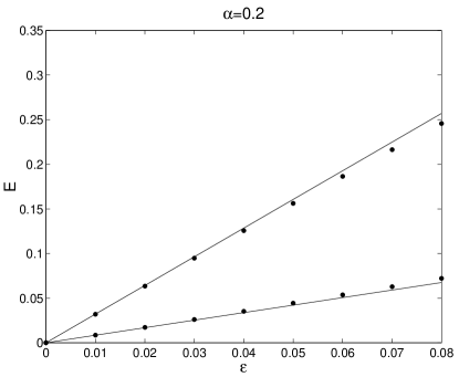
(c)	(d)
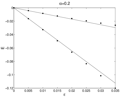
(e)	(f)

Figure 4: Dependence of $E=\varepsilon\lambda_{1}$ and $E=\varepsilon\lambda_{2}$ with respect to $\varepsilon$ for two different values of $\alpha$. (a,b) correspond to in-phase 3-site breathers, (c,d) to out-of-phase 3-site breathers with the impurity at the center and (e,f) to the same as before but with the impurity at the edge. All the solutions stand for a hard $\phi^{4}$ potential and $\omega_{\mathrm{b}}=1.3$. Points represent numerical solutions and lines analytical ones.

(a)	(b)

Figure 5: Dependence of $E=\varepsilon\lambda_{1}$ for a 2-site and a 3-site breather with an impurity at the coupling located at the edge. All the solutions stand for a Morse potential and $\omega_{\mathrm{b}}=0.8$. Points correspond to numerical solutions and lines to analytical ones.

6 Multibreathers and phonobreathers with an impurity

A multibreather is obtained from the anticontinuous limit when a number of contiguous oscillators are excited. If all the oscillators are excited it is called a phonobreather. Provided that a multibreather does not include the oscillators at the borders, the modified coupling matrix of a N-site multibreather is identical to the one of a phonobreather with fixed ends. Therefore, we can study both cases simultaneously. We cannot obtain analytical expressions for the eigenvalues of the perturbation matrixes, but we have been able to demonstrate their stability properties.

When the number of oscillator of a multibreather increases, the degree of the characteristic polynomial also increases and an analytical evaluation of its roots is not possible. However, in the case of a homogenous system, the eigenvalues can be calculated because the eigenvectors equation of the system is equivalent to the dynamical equations of a linear lattice of oscillators, as shown in [6]. Although this analogy might be suggested in our case, the only information available for the eigenvalues would be the dependence on the parameters of a localized eigenvalues and only in an infinite lattice.

Thus, we can only obtain qualitative results about the spectrum of the matrix $Q$ for a phonobreather (or N-site multibreather). In particular, we show that the stability properties of the system with an impurity are the same as an homogeneous system. In order to do that, we will make use of some congruence properties of symmetric matrices [8].

Two symmetric matrices $A$ and $B$ are congruent if they can be transformed each other through elementary transformations: $B=PAP^{t}$. The inertia of a matrix is defined as $\mathrm{In}(A)=\{i_{+}(A),i_{-}(A),i_{0}(A)\}$ where $i_{+}$, $i_{-}$, $i_{0}$ denote, respectively, the number of positive, negative and zero eigenvalues of $A$. Sylvester’s inertia law establishes that the inertia of two congruent matrices are the same [9]. In consequence, it is enough to diagonalize a matrix using elementary transformations to obtain its inertia. The diagonal matrix has the structure called first canonical form:

$$D=\{\underbrace{1,\ldots,1}_{i_{+}\ \textrm{times}},\underbrace{-1,\ldots,-1}_{i_{-}\ \textrm{times}},\underbrace{0,\ldots,0}_{i_{0}\ \textrm{times}}\}$$ (15)

We analyze below the stability properties of phonobreathers with different boundary conditions and an inhomogeneity at the on-site potential. Let us recall that, in the homogeneous case, the inertia of $Q$ is, for an in-phase breather, $\mathrm{In}(Q)=\{N-1,0,1\}$ and, for an out-of-phase (staggered) breather, $\mathrm{In}(Q)=\{0,N-1,1\}$, with $N$ being the number of system particles. We will show that the inertia does not change when an impurity is introduced.

Furthermore, the only multibreathers that can be stable are those that vibrate in-phase or staggered, as demonstrated in B.

6.1 Multibreathers and phonobreathers with free/fixed ends boundary conditions

If the impurity is supposed to be located at $n=c$, the elements of the perturbation matrix $Q^{F0}$ for an in-phase multibreather, can be written as:

$$Q^{F0}_{nm}=2\delta_{n,m}[1+(\eta\varphi-1)\delta_{n,c}+(\eta/\varphi-1)/2\delta_{|n-c|,1}-(\delta_{n,1}+\delta_{n,N})/2]-$$

$$-\delta_{n,m+1}[1-(\eta+1)(\delta_{n,c}+\delta_{n,c+1})]-\delta_{n,m-1}[1-(\eta+1)(\delta_{n,c}+\delta_{n,c-1})].$$ (16)

This matrix is transformed into a diagonal matrix through $D=PQP^{t}$, where

$$P_{nm}=[\delta_{[\frac{m}{n}],0}+\delta_{n,m}][1+\delta_{[\frac{m}{c}],0}\delta_{n,c-1}(\sqrt{\varphi/\eta}-1)+\delta_{m,c}\delta_{[\frac{n}{c}],0}/\varphi+$$

$$\hbox to0.0pt{\hss${}+{}$}\delta_{n,c-1}((\sqrt{\varphi/\eta}-1)\delta_{[\frac{m}{c}],0}+(1/\sqrt{\varphi\eta}-1)\delta_{m,c})],$$ (17)

where $[\cdot]$ denotes the integer part. $D_{nm}=\delta_{n,m}(1-\delta_{n,N})$. In consequence, $\mathrm{In}(Q^{F0})=\{N-1,0,1\}$ and all of the eigenvalues are positive except for one which is zero.

The perturbation matrix for the out-of-phase breather is given by:

$$Q^{F\pi}_{nm}=-2\gamma_{0}\delta_{n,m}[1+(\gamma\varphi-1)\delta_{n,c}+(\gamma/\varphi-1)/2\delta_{|n-c|,1}-(\delta_{n,1}+\delta_{n,N})/2]-$$

$$+\gamma_{0}\delta_{n,m+1}[1-(\gamma_{0}+1)(\delta_{n,c}+\delta_{n,c+1})]+\gamma_{0}\delta_{n,m-1}[1-(\gamma/\gamma_{0}+1)(\delta_{n,c}+\delta_{n,c-1})],$$ (18)

which transform into the diagonal matrix $D_{nm}=-\delta_{n,m}(1-\delta_{n,N})$ through the transformation matrix

$$P_{nm}=[\delta_{[\frac{m}{n}],0}+\delta_{n,m}][1+\delta_{[\frac{m}{c}],0}\delta_{n,c-1}(\sqrt{\varphi/\gamma}-1)+\delta_{m,c}\delta_{[\frac{n}{c}],0}/\varphi+$$

$$\hbox to0.0pt{\hss${}+{}$}\delta_{n,c-1}((\sqrt{\varphi/\gamma}-1)\delta_{[\frac{m}{c}],0}+(1/\sqrt{\varphi\gamma}-1)\delta_{m,c})].$$ (19)

The inertia of the stability matrix is given by $\mathrm{In}(Q^{F\pi})=\{0,N-1,1\}$ and, in consequence, it has all its eigenvalues negatives except for the null one.

Figure 6 shows the numerical values of the eigenvalues and confirms the results stated previously.

(a)	(b)
(c)

Figure 6: Dependence of the eigenvalues of the perturbation matrix with respect to the impurity parameter $\alpha$ for a phonobreather with free/fixed ends boundary condition. (a) and (b) corresponds to the Morse potential and $\omega_{\mathrm{b}}=0.8$ while (c) to a hard $\phi^{4}$ potential. (a) and (c) corresponds to a in-phase breather and (b) to a staggered one.

6.2 Periodic boundary conditions

The diagonalization of $Q$ is now very difficult. We will make use instead of a theorem due to Weyl [8] to obtain the inertia of the matrix. This theorem establishes that, if the eigenvalues of a matrix are arranged in the following order: $\lambda_{1}\leq\lambda_{2}\leq\ldots\leq\lambda_{N}$ then, the k-th eigenvalue of the sum of two matrices holds:

$$\lambda_{k}(A)+\lambda_{1}(B)\leq\lambda_{k}(A+B)\leq\lambda_{k}(A)+\lambda_{N}(B).$$ (20)

This theorem can be particularized for our case if we denote as $Q^{P0}$ and $Q^{P\pi}$ to the periodic boundary conditions matrices and define $Q^{P}=Q^{F}+\Delta$, where $Q^{F}$ is the perturbation matrix with free boundary conditions. By making $A\equiv Q^{F}$ and $B\equiv\Delta$ we can apply Weyl’s theorem.

For a phonobreather in-phase,

$$Q^{P0}_{nm}=2\delta_{n,m}[1+(\eta\varphi-1)\delta_{n,c}+(\eta/\varphi-1)/2\delta_{|n-c|,1}]-(\delta_{n,1}\delta_{m,N}+\delta_{n,N}\delta_{m,1})-$$

$$-\delta_{n,m+1}[1-(\eta+1)(\delta_{n,c}+\delta_{n,c+1})]-\delta_{n,m-1}[1-(\eta+1)(\delta_{n,c}+\delta_{n,c-1})],$$ (21)

and, in consequence,

$$\Delta_{n,m}=\delta_{n,m}(\delta_{n,1}+\delta_{n,N})-(\delta_{n,1}\delta_{m,N}+\delta_{n,N}\delta_{m,1}).$$ (22)

The spectrum of $\Delta$ is given by $\mathrm{spec}(\Delta)=\{0,2\}$ where $\lambda_{1}(\Delta)=0$ has multiplicity $N-1$ and $\lambda_{N}(\Delta)=2$ has multiplicity 1. Thus, particularizing (20) for $k=1$:

$$\lambda_{1}(Q^{F0})+\lambda_{1}(\Delta)\leq\lambda_{1}(Q^{P0})\leq\lambda_{1}(Q^{F0})+\lambda_{N}(\Delta).$$ (23)

As $\lambda_{1}(Q^{F0})=0$, $\lambda_{1}(Q^{F0})\in[0,2]$. If $k=2$ is taken in (20), $\lambda_{2}(Q^{P0})\geq\lambda_{2}(Q^{F0})+\lambda_{1}(\Delta)$. As $\lambda_{2}(Q^{F0})>0$ then $\lambda_{2}(Q^{P0})>0$. In consequence, $Q^{P0}$ has $N-1$ positive eigenvalues and one which is greater or equal to zero.

The steps for an out-of-phase multibreather are similar to the in-phase case, except that $k=N$ is taken in (20). Thus, it is straightforward to show that $Q^{P\pi}$ has all its eigenvalues negatives except for one of them which is smaller or equal to zero.

Figure 7 shows the numerical values of the eigenvalues and confirms the previously stated results.

(a)	(b)
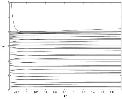
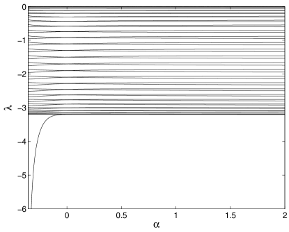
(c)

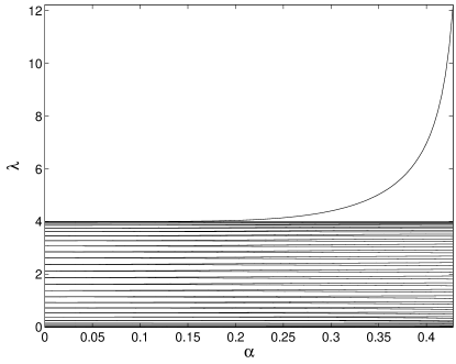
Figure 7: Dependence of the eigenvalues of the perturbation matrix with respect to the impurity parameter $\alpha$ for a phonobreather with periodic boundary condition. (a) and (b) corresponds to Morse potential and $\omega_{\mathrm{b}}=0.8$ while (c) to a hard $\phi^{4}$ potential. (a) and (c) corresponds to a in-phase breather and (b) to a staggered one.

Let us remark that for $N$ odd there appear, in a similar fashion to the homogeneous case, parity instabilities due to the breaking of the breather pattern. Figure 8 shows the dependence of the eigenvalues of $Q$ with respect to $\alpha$ in this case. It can be observed the existence of a positive eigenvalue of constant value. It was demonstrated in [10] that in a homogeneous lattice, this eigenvalue is $4\gamma_{0}/3$ in an infinite lattice. This value does not change when an impurity is introduced as it is due to a border effect.

(a)	(b)

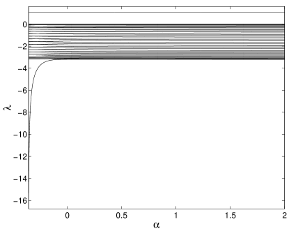
Figure 8: Dependence of the eigenvalues of the perturbation matrix with respect to the impurity parameter $\alpha$ for a Morse potential and $\omega_{\mathrm{b}}=0.8$ in the case of staggered (a) phonobreathers and (b) dark breathers with periodic boundary conditions. The existence of an isolated positive eigenvalue $\lambda=4\gamma_{0}/3\approx 1.07$ is observed.

6.3 Inhomogeneity at the coupling constant

In this case, the perturbation matrix is equivalent to the one corresponding to an inhomogeneity implemented at the on-site potential with the changes $\varphi=1$ and $\eta=\gamma=1+\beta/2$. In consequence, the results are qualitatively the same in both cases.

7 Dark breathers with an impurity

A particular case of multibreathers in which all the particles of the lattice are excited except one is called a dark breather [11, 12]. In the case that there are $p$ adjacent sites with no vibration, we deal with a p-site dark breather. For the sake of simplicity we will consider 1-site dark breathers as the generalization to p-site dark breathers is straightforward.

It is worth noticing that if the impurity is located at the dark site, the perturbation matrix turns into the homogeneous one. In consequence, the only way to introduce a modification in the perturbation matrix is to suppose the impurity adjacent to the dark site.

For an in-phase breather, the perturbation matrix is given by (notice that the $c+1$ row and column are removed):

$$Q^{D0}_{nm}=2\delta_{n,m}[1+(\eta\varphi-1)\delta_{n,c}+(\eta/\varphi-1)/2\delta_{n,c-1}+(b-1)(\delta_{n,1}+\delta_{n,N})/2]-$$

$$-\delta_{n,m+1}[1-(\eta+1)\delta_{n,c-1}]-\delta_{n,m-1}[1-(\eta+1)\delta_{n,c-1}]-b(\delta_{1,N}+\delta_{1,N}),$$ (24)

where $b=0$ for fixed/free ends and $b=1$ for periodic boundary conditions. If $b=0$ the perturbation matrix is block diagonal, being the lower block the matrix of a phonobreather with fixed/free ends boundary conditions and $N-(c+1)$ particles. The upper block is a matrix $Q_{1}$ with positive eigenvalues except for a null one. In consequence, the inertia of the perturbation matrix for $b=0$ is $\{N-2,0,2\}$. The existence of two zero eigenvalues makes it impossible to determine the stability through the theorem as, to first order of the perturbation, the degeneration is not raised. This result was also obtained in the homogeneous case.

For $b=1$, i.e. periodic boundary conditions, the perturbation matrix can be transformed into $Q_{1}$ through row/columns interchange. This transformation lets the characteristic polynomial invariant. In consequence, the matrix has $N-1$ positive eigenvalues and a null one.

The perturbation matrix of a staggered dark breather is

$$Q^{D\pi}_{nm}=-2\gamma_{0}\delta_{n,m}[1+(\gamma\varphi-1)\delta_{n,c}+(\gamma/\varphi-1)/2\delta_{n,c-1}+(b-1)(\delta_{n,1}+\delta_{n,N})/2]-$$

$$\hbox to0.0pt{\hss${}-{}$}\gamma_{0}\delta_{n,m+1}[1-(\gamma/\gamma_{0}+1)\delta_{n,c-1}]$$

$$\hbox to0.0pt{\hss${}-{}$}\gamma_{0}\delta_{n,m-1}[1-(\gamma/g_{0}+1)\delta_{n,c-1}]-b\gamma_{0}(\delta_{1,N}+\delta_{1,N}).$$ (25)

It can be shown straightforwardly that $\mathrm{In}(Q^{D\pi}(b=0))=\{0,N-2,2\}$ and $\mathrm{In}(Q^{D\pi}(b=1))=\{0,N-1,1\}$. In the case of $N$ odd and $b=1$, parity instabilities also occur (see Figure 8).

Figure 9 shows the eigenvalues for a dark breather with periodic boundary conditions.

(a)	(b)
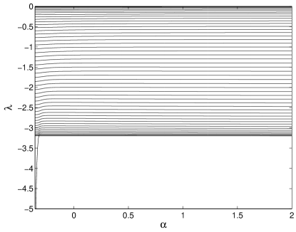
(c)

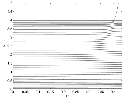
Figure 9: Dependence of the eigenvalues of the perturbation matrix with respect to the impurity parameter $\alpha$ for a dark breather with free/fixed ends boundary condition. (a) and (b) corresponds to Morse potential and $\omega_{\mathrm{b}}=0.8$ while (c) to a hard $\phi^{4}$ potential. (a) and (c) corresponds to a in-phase breather and (b) to a staggered one.

8 Conclusions

The Multibreathers Stability Theorem [6] provides with a method for obtaining the perturbation matrix $Q$ from the anticontinuous limit of any multibreather at low coupling in Klein-Gordon systems. The stability depends on the signs of the eigenvalues of $Q$, the hardness/softnes of the on-site potential and the sign of the coupling parameter (i.e., the attractiveness or repulsiveness of the coupling). In this paper we apply the MST to systems with an impurity either at the on-site potential or the coupling constants, the first case being equivalent to an impurity at the masses.

Using analytical methods we have been able to obtain the eigenvalues of $Q$ for 2-site and 3-site breathers and compare them with numerical results showing an excellent agreement. For larger multibreathers, phonobreathers and dark breathers we have obtained analytically the signs of the $Q$-eigenvalues and checked them numerically. In all cases, although the values of the eigenvalues change, the stability properties of the system with an impurity coincides with the ones of the homogeneous system.

The necessity of either an in-phase pattern or an out-of-phase one for the stability of a multibreather in the homogenous system, as it was conjectured in Ref. [6], has also been demonstrated.

Appendix A Analytical calculation of parameters

The aim of this appendix is to calculate analytically the parameters $\eta_{nm}$, $\gamma_{nm}$, $\varphi_{nm}$ defined in Section 3 as:

$$\eta_{nm}=\frac{J_{nm}}{\sqrt{J_{nn}J_{mm}}}>0,\qquad\gamma_{nm}=-\frac{J^{\prime}_{nm}}{\sqrt{J_{nn}J_{mm}}}>0,\qquad\varphi_{nm}=\sqrt{\frac{J_{mm}}{J_{nn}}}>0,$$ (26)

with

$$J_{nm}=\int_{-T/2}^{T/2}\,\dot{u}_{n}(t)\,\dot{u}_{m}(t)\,\mathrm{d}t\,,\qquad J^{\prime}_{nm}=\int_{-T/2}^{T/2}\,\dot{u}_{n}(t)\,\dot{u}_{m}(t+T/2)\,\mathrm{d}t\,.$$ (27)

Analytical calculation of these integrals is rather difficult. In order to overcome this difficulty, solutions $u_{n}(t)$ are expressed as a Fourier series expansion:

$$u_{n}(t)=z_{0,n}+2\sum_{k=1}^{\infty}z_{k,n}\cos(k\omega_{\mathrm{b}}\,t),$$ (28)

and the integrals turn into series:

$$J_{nm}=4\pi\omega_{\mathrm{b}}\sum_{k=1}^{\infty}k^{2}z_{k,n}z_{k,m},\qquad J^{\prime}_{nm}=4\pi\omega_{\mathrm{b}}\sum_{k=1}^{\infty}(-1)^{k}k^{2}z_{k,n}z_{k,m}.$$ (29)

In consequence, the theorem parameters can be expressed as a function of the Fourier coefficients of the solution. In the case of the Morse potential, the sum can be performed and a closed expression is obtained.

A.1 Morse potential

The Morse potential has the expression $V(u_{n})=(1+\alpha_{n})(\exp(-u_{n})-1)^{2}/2$, and the orbits of the equation $\ddot{u}_{n}+V^{\prime}(u_{n})=0$ are given by [6]:

$$u_{n}(t)=\log\frac{1\mp\sqrt{1-(\omega_{\mathrm{b}}/\omega_{\mathrm{n}})^{2}}\cos\omega_{\mathrm{b}}\,t}{(\omega_{\mathrm{b}}/\omega_{\mathrm{n}})^{2}}\,,$$ (30)

The minus sign corresponds to $u_{n}(0)>0$ and the plus sign to $u_{n}(0)<0$ with $\omega_{\mathrm{n}}=\sqrt{1+\alpha_{n}}$. The Fourier coefficients are:

$$z_{0,n}=\log\frac{\omega_{\mathrm{n}}+\omega_{\mathrm{b}}}{2\omega_{\mathrm{b}}^{2}}\quad;\quad z_{k,n}=-\,\frac{\rho_{k}}{k}\left(\frac{\omega_{\mathrm{n}}-\omega_{\mathrm{b}}}{\omega_{\mathrm{n}}+\omega_{\mathrm{b}}}\right)^{k/2}\,,$$ (31)

with $\rho_{k}=(-1)^{k+1}$ if $u_{n}(0)>0$ and $\rho_{k}=-1$ if $u_{n}(0)<0$. Thus,

$$J_{nm}=4\pi\omega_{\mathrm{b}}\sum_{k=1}^{\infty}\left[\frac{(\omega_{\mathrm{n}}-\omega_{\mathrm{b}})(\omega_{\mathrm{m}}-\omega_{\mathrm{b}})}{(\omega_{\mathrm{n}}+\omega_{\mathrm{b}})(\omega_{\mathrm{m}}+\omega_{\mathrm{b}})}\right]^{k/2},$$ (32)

$$J^{\prime}_{nm}=4\pi\omega_{\mathrm{b}}\sum_{k=1}^{\infty}\left[-\frac{(\omega_{\mathrm{n}}-\omega_{\mathrm{b}})(\omega_{\mathrm{m}}-\omega_{\mathrm{b}})}{(\omega_{\mathrm{n}}+\omega_{\mathrm{b}})(\omega_{\mathrm{m}}+\omega_{\mathrm{b}})}\right]^{k/2}.$$ (33)

The sums are geometric series whose ratios have absolute values smaller than one. In consequence, they can be easily summed and the resulting values of $J$ and $J^{\prime}$ are:

$$J_{nm}=4\pi\omega_{\mathrm{b}}\frac{\sqrt{(\omega_{\mathrm{n}}-\omega_{\mathrm{b}})(\omega_{\mathrm{m}}-\omega_{\mathrm{b}})}}{\sqrt{(\omega_{\mathrm{n}}+\omega_{\mathrm{b}})(\omega_{\mathrm{m}}+\omega_{\mathrm{b}})}-\sqrt{(\omega_{\mathrm{n}}-\omega_{\mathrm{b}})(\omega_{\mathrm{m}}-\omega_{\mathrm{b}})}},$$ (34)

$$J^{\prime}_{nm}=4\pi\omega_{\mathrm{b}}\frac{\sqrt{(\omega_{\mathrm{n}}-\omega_{\mathrm{b}})(\omega_{\mathrm{m}}-\omega_{\mathrm{b}})}}{\sqrt{(\omega_{\mathrm{n}}+\omega_{\mathrm{b}})(\omega_{\mathrm{m}}+\omega_{\mathrm{b}})}+\sqrt{(\omega_{\mathrm{n}}-\omega_{\mathrm{b}})(\omega_{\mathrm{m}}-\omega_{\mathrm{b}})}}.$$ (35)

Then, applying equation (26), the theorem parameters are:

$$\eta_{nm}=\frac{2\omega_{\mathrm{b}}}{\sqrt{(\omega_{\mathrm{n}}+\omega_{\mathrm{b}})(\omega_{\mathrm{m}}+\omega_{\mathrm{b}})}-\sqrt{(\omega_{\mathrm{n}}-\omega_{\mathrm{b}})(\omega_{\mathrm{m}}-\omega_{\mathrm{b}})}},$$ (36)

$$\gamma_{nm}=\frac{2\omega_{\mathrm{b}}}{\sqrt{(\omega_{\mathrm{n}}+\omega_{\mathrm{b}})(\omega_{\mathrm{m}}+\omega_{\mathrm{b}})}+\sqrt{(\omega_{\mathrm{n}}-\omega_{\mathrm{b}})(\omega_{\mathrm{m}}-\omega_{\mathrm{b}})}},$$ (37)

$$\varphi_{nm}=\sqrt{\frac{\omega_{\mathrm{m}}-\omega_{\mathrm{b}}}{\omega_{\mathrm{n}}-\omega_{\mathrm{b}}}}.$$ (38)

A.2 $\phi^{4}$ potential

This potential is given by $V(u_{n})=(1+\alpha_{n})u_{n}^{2}/2-su_{n}^{4}/4$, with $s=\pm 1$. The sign of $s$ allow us to define two different cases:

A.2.1 Hard $\phi^{4}$ potential. $s=+1$.

The orbit of a hard oscillator is given by:

$$u_{n}(t)=\pm\omega_{\mathrm{n}}\sqrt{\frac{2\kappa_{n}^{2}}{1-2\kappa_{n}^{2}}}\mathrm{cn}\left(\frac{\omega_{\mathrm{n}}t}{\sqrt{1-2\kappa_{n}^{2}}},\kappa_{n}\right)$$

$$\hbox to0.0pt{\hss${}={}$}\pm\omega_{\mathrm{n}}\sqrt{\frac{2\kappa_{n}^{2}}{1-2\kappa_{n}^{2}}}\mathrm{cn}\left(\frac{2K(\kappa_{n})}{\pi}\omega_{\mathrm{b}}\,t,\kappa_{n}\right),$$ (39)

where $\mathrm{cn}$ is a Jacobi elliptic function of modulus $\kappa_{n}$ and $K(\kappa_{n})$ is the complete elliptic integral of the first kind defined as:

$$K(\kappa)=\int_{0}^{\pi/2}\,\frac{\mathrm{d}x}{\sqrt{1-\kappa^{2}\sin^{2}x}}\,.$$ (40)

The breather frequency $\omega_{\mathrm{b}}$ is related to the modulus $\kappa_{n}$ through:

$$\omega_{\mathrm{b}}=\frac{\pi\omega_{\mathrm{n}}}{2\sqrt{1-2\kappa_{n}^{2}}K(\kappa_{n})}.$$ (41)

The elliptic function can be expanded into a Fourier series and it is obtained [13]:

$$z_{2\nu+1,n}=\pm\frac{\pi}{K(\kappa_{n})}\sqrt{\frac{2}{1-2\kappa_{n}^{2}}}\,\frac{q_{n}^{\nu+1/2}}{1+q_{n}^{2\nu+1}},\qquad\nu=0,1,2,\ldots.$$ (42)

$q_{n}$ is the Nome and is defined as

$$q_{n}=\exp(-\pi K(\sqrt{1-\kappa^{2}_{n}})/K(\kappa_{n})).$$ (43)

Thus, $J_{nm}$ is given by (note that $J^{\prime}=-J$ as the potential is even):

$$J_{nm}=\frac{8\pi^{3}\omega_{\mathrm{b}}}{K(\kappa_{n})K(\kappa_{m})}\sqrt{\frac{q_{n}q_{m}}{(1-2\kappa_{n}^{2})(1-2\kappa_{m}^{2})}}\sum_{\nu=0}^{\infty}\frac{(2\nu+1)^{2}(q_{n}q_{m})^{\nu}}{(1+q_{n}^{2\nu+1})(1+q_{m}^{2\nu+1})},$$ (44)

and, in consequence,

$$\eta_{nm}=\frac{\displaystyle\sum_{\nu=0}^{\infty}\frac{(2\nu+1)^{2}(q_{n}q_{m})^{\nu}}{(1+q_{n}^{2\nu+1})(1+q_{m}^{2\nu+1})}}{\displaystyle\sqrt{\sum_{\nu=0}^{\infty}\left(\frac{(2\nu+1)q_{n}^{\nu}}{1+q_{n}^{2\nu+1}}\right)^{2}}\sqrt{\sum_{\nu=0}^{\infty}\left(\frac{(2\nu+1)q_{m}^{\nu}}{1+q_{m}^{2\nu+1}}\right)^{2}}}\,,$$ (45)

$$\varphi_{nm}=\frac{\displaystyle\omega_{\mathrm{m}}K(\kappa_{n})}{\displaystyle\omega_{\mathrm{n}}K(\kappa_{m})}\sqrt{\frac{\displaystyle(1-2\kappa_{n}^{2})\sum_{\nu=0}^{\infty}\left(\frac{(2\nu+1)q_{m}^{\nu}}{1+q_{m}^{2\nu+1}}\right)^{2}}{\displaystyle(1-2\kappa_{m}^{2})\sum_{\nu=0}^{\infty}\left(\frac{(2\nu+1)q_{n}^{\nu}}{1+q_{n}^{2\nu+1}}\right)^{2}}}\,.$$ (46)

A.2.2 Soft $\phi^{4}$ potential. $s=-1$.

Now, the orbit of an oscillator is given by:

$$u_{n}(t)=\pm\omega_{\mathrm{n}}\sqrt{\frac{2\kappa_{n}^{2}}{1+\kappa_{n}^{2}}}\mathrm{cd}\left(\frac{\omega_{\mathrm{n}}t}{\sqrt{1+\kappa_{n}^{2}}},\kappa_{n}\right)=\pm\omega_{\mathrm{n}}\sqrt{\frac{2\kappa_{n}^{2}}{1+\kappa_{n}^{2}}}\mathrm{cd}\left(\frac{2K(\kappa_{n})}{\pi}\omega_{\mathrm{b}}\,t,\kappa_{n}\right),$$ (47)

where $\mathrm{cd}$ is another elliptic function. Now, the breather frequency $\omega_{\mathrm{b}}$ and the modulus $\kappa_{n}$ are related through:

$$\omega_{\mathrm{b}}=\frac{\pi\omega_{\mathrm{n}}}{2\sqrt{1+\kappa_{n}^{2}}K(\kappa_{n})}.$$ (48)

Following [13], the Fourier coefficients can be obtained:

$$z_{2\nu+1,n}=\pm\frac{\pi}{K(\kappa_{n})}\sqrt{\frac{2}{1+\kappa_{n}^{2}}}\,\frac{q_{n}^{\nu+1/2}}{1-q_{n}^{2\nu+1}},$$ (49)

and, in consequence,

$$J_{nm}=\frac{8\pi^{3}\omega_{\mathrm{b}}}{K(\kappa_{n})K(\kappa_{m})}\sqrt{\frac{q_{n}q_{m}}{(1+\kappa_{n}^{2})(1+\kappa_{m}^{2})}}\sum_{\nu=0}^{\infty}\frac{(2\nu+1)^{2}(q_{n}q_{m})^{\nu}}{(1-q_{n}^{2\nu+1})(1-q_{m}^{2\nu+1})},$$ (50)

$$\eta_{nm}=\frac{\displaystyle\sum_{\nu=0}^{\infty}\frac{(2\nu+1)^{2}(q_{n}q_{m})^{\nu}}{(1-q_{n}^{2\nu+1})(1-q_{m}^{2\nu+1})}}{\displaystyle\sqrt{\sum_{\nu=0}^{\infty}\left(\frac{(2\nu+1)q_{n}^{\nu}}{1-q_{n}^{2\nu+1}}\right)^{2}}\sqrt{\sum_{\nu=0}^{\infty}\left(\frac{(2\nu+1)q_{m}^{\nu}}{1-q_{m}^{2\nu+1}}\right)^{2}}}\,,$$ (51)

$$\varphi_{nm}=\frac{\displaystyle\omega_{\mathrm{m}}K(\kappa_{n})}{\displaystyle\omega_{\mathrm{n}}K(\kappa_{m})}\sqrt{\frac{\displaystyle(1+\kappa_{n}^{2})\sum_{\nu=0}^{\infty}\left(\frac{(2\nu+1)q_{m}^{\nu}}{1-q_{m}^{2\nu+1}}\right)^{2}}{\displaystyle(1+\kappa_{m}^{2})\sum_{\nu=0}^{\infty}\left(\frac{(2\nu+1)q_{n}^{\nu}}{1-q_{n}^{2\nu+1}}\right)^{2}}}\,.$$ (52)

Appendix B Demonstration of the necessity of an in-phase or out-of-phase pattern for the stability of multibreathers

It was shown in Ref. [6] that a multibreather with nearest neighbour coupling and whose vibration pattern is neither in-phase nor out-of-phase is unstable independently of the hardness/sotftness of the on-site potential and the sign of the coupling constant. However, this fact was not demonstrated.

In this appendix, we will demonstrate the last assertion by making use of a consequence of Sylvester’s inertia law, called Sylvester’s Theorem [8]. It establishes that, for a positive definite matrix, the principal minors are positive, for a negative definite one, the principal minors alternate their signs when the dimension increases by one and, finally, a matrix is not definite when none of the last conditions are fulfilled.

Let us suppose an homogeneous lattice. If the pattern of vector $\sigma$ is different from the in-phase or staggered ones, there is always a sequence $\{-1,1,1\}$ or $\{1,-1,-1\}$ on it. It is easy to show that in both cases, the perturbation matrix has the form:

$$Q=\left[\begin{array}[]{ccc}\ddots&&\\ &Q_{0}&\\ &&\ddots\end{array}\right],$$ (53)

with

$$Q^{0}=\left[\begin{array}[]{ccc}-\gamma_{0}&\gamma_{0}&0\\ \gamma&1-\gamma_{0}&0\\ 0&1&\bullet\end{array}\right],$$ (54)

where $\bullet$ is a number that depends on the phase of the particle adjacent to the pattern breaking sequence. As the spectrum of $Q$ is invariant under rows/columns exchanges, the block $Q^{0}$ can be placed at $Q_{1,1}$, and Sylvester’s theorem can be applied to $Q^{0}$. The 1st order minor is $M^{(1)}=Q^{0}_{1,1}=-\gamma_{0}<0$, and the 2nd order one, $M^{(2)}=Q^{0}_{1,1}Q^{0}_{2,2}-Q^{0}_{1,2}Q^{0}_{2,1}=-\gamma_{0}<0$. In consequence, the matrix is not definite and there are positive and negative eigenvalues.

Let us suppose now that an impurity is introduced in the pattern breaking sites. The matrices for impurities in the first, second and third sites are (note that we only consider the first $(2\times 2)$ submatrix as the result is independent on the third row/column), respectively:

$$Q^{0}_{1}=\left[\begin{array}[]{ccc}-\gamma\varphi&\gamma\\ \gamma&-\gamma/\varphi+1\end{array}\right],$$ (57)

$$\hbox to0.0pt{\hss${}Q^{0}_{2}{}$}=\left[\begin{array}[]{ccc}-\gamma/\varphi&\gamma\\ \gamma&(\eta-\gamma)/\varphi\end{array}\right],\;Q^{0}_{3}=\left[\begin{array}[]{ccc}-\gamma_{0}&\gamma_{0}\\ \gamma_{0}&\eta/\varphi-\gamma_{0}\end{array}\right],$$ (62)

and the corresponding minors are: $\{M^{(1)}_{1}=-\gamma\varphi,M^{(2)}_{1}=-\gamma\varphi\}$, $\{M^{(1)}_{2}=-\gamma/\varphi,M^{(2)}_{2}=-\gamma\eta\}$, $\{M^{(1)}_{3}=-\gamma_{0},M^{(2)}_{3}=-\gamma_{0}\eta/\varphi\}$. In consequence, the matrices are not definite.

References

- [1] RS MacKay and S Aubry. Proof of existence of breathers for time-reversible or Hamiltonian networks of weakly coupled oscillators. Nonlinearity, 7:1623, 1994.
- [2] S Aubry. Breathers in nonlinear lattices: Existence, linear stability and quantization. Physica D, 103:201, 1997.
- [3] JL Marín, S Aubry, and LM Floría. Intrinsic Localized Modes: Discrete breathers. Existence and linear stability. Physica D, 113:283, 1998.
- [4] RS MacKay and JA Sepulchre. Stability of discrete breathers. Physica D, 119:148, 1998.
- [5] JL Marín. Intrinsic Localized Modes in nonlinear lattices. PhD Thesis, University of Zaragoza (Spain), June 1997.
- [6] JFR Archilla, J Cuevas, B Sánchez-Rey, and A Álvarez. Demonstration of the stability or instability of multibreathers at low coupling. Physica D, 180:235, 2003.
- [7] J Cuevas, F Palmero, J F R Archilla, and F R Romero. Moving discrete breathers in a Klein–Gordon chain with an impurity. J. Phys. A: Math. and Gen., 35:10519, 2002.
- [8] RA Horn and CR Johnson. Matrix Analysis. Cambridge University Press, 1985.
- [9] JJ Sylvester. A demonstration of the theorem that every homogeneous quadratic polynomial is reducible by real orthogonal substitutions to the form of a sum of positive and negative squares. Phil. Mag., IV:138, 1852.
- [10] J Cuevas. Localization and energy transfer in anharmonic inhomogeneus lattices. PhD Dissertation, Physics Faculty, University of Sevilla (Spain), 2003.
- [11] A Álvarez, JFR Archilla, J Cuevas, and FR Romero. Dark breathers in Klein-Gordon lattices. Band analysis of their stability properties. New Jornal of Physics, 4:72, 2002.
- [12] AM Morgante, M Johannson, G Kopidakis, and S Aubry. Standing waves instabilities in a chain of nonlinear coupled oscillators. Physica D, 162:53, 2002.
- [13] M Abramowitz and IA Stegun. Handbook of mathematical functions. Dover, New York, 1965.