Correlations among the Riemann zeros: Invariance, resurgence, prophecy and self-duality

Abstract

We present a conjecture describing new long range correlations among the Riemann zeros leading to 3 principal features: (i) The spectral auto-correlation is invariant w.r.t. the averaging window. (ii) Resurgence occurs wherein the lowest zeros appear in all auto-correlations. (iii) Suitably defined correlations lead to predictions (prophecy) of new zeros. This conjecture is supported by analytical arguments and confirmed by numerical calculations using $10^{22}$ zeros computed by Odlyzko. The results lead to a self-duality of the Riemann spectrum similar to the quantum-classical duality observed in billiards.

I Introduction

The Riemann zeta function is

$$\zeta(s)=\sum\limits_{n=1}^{\infty}\frac{1}{n^{s}}=\prod\limits_{p}(1-p^{-s})^{-1}$$

with product over all prime numbers $p$. The Riemann zeta function has a simple pole at $s=1$. Besides the trivial zeros at $s=-2,-4,-6,\cdots$, the Riemann hypothesis (RH) states that all the nontrivial zeros are distributed on line as $\frac{1}{2}\pm it_{n}$ with $t_{n}>0$ Conrey . The Riemann zeta function and its zeros have been studied for over a century Edwards ; Titch ; Berry140 ; Berry175 ; Keating96 ; Berry306 ; Berry307 ; Keating ; Connors ; Odly ; Bohigas01 ; Leboeuf01 ; Zyl ; Sakhr03 ; Bogomolny03 ; Leboeuf04 . The RH still remains unproven and presents a major mathematical challenge Sabbagh .

Motivated by the Hilbert-Polya conjecture of the existence of a Hamiltonian whose quantum spectrum is comprised of the set $\{t_{n}\}$ as the spectra, there has been a continuing quest to find such a Hamiltonian since it would prove the RH. Attempts have been made to construct certain Hamiltonian such as that with a fractal potential Wu93 for the Riemann zeros (RZ). For a brief review about Hamiltonians and prime numbers, see Rosu .

The RZ $\{\frac{1}{2}\pm it_{n}\}$ can also be considered as a model spectrum for arithmetic or quantum chaos Sarnak . It is widely believed that the ordinates $\{t_{n}\}$ of the RZ can be interpreted as the quantum spectrum of a chaotic system which does not have time reversal symmetry Berry154 ; Berry307 though other interpretations are also possible. The most notable result in support of this notion is that of Montgomery Montgomery who showed that the spectral correlation function $R_{2}(s)$ of the RZ is identical with that of a Gaussian Unitary Ensemble (GUE) which describes a chaotic system with no time-reversal symmetry in random matrix theory. This result has led to a line of inquiry which studies the statistics and correlations among the RZ. The merit of this approach is that the properties of the RZ will lead to insights into other systems where the classical dynamics is well established. These are motivated by the analog of the Riemann zeta function with Gutzwiller’s trace formula and the dynamic zeta function of chaotic systems.

In this paper, we present a conjecture which reveals new long range correlations among the RZ, obtained from a study of the auto-correlation of a smoothed Riemann spectrum. Several new properties emerge: (i) The spectral auto-correlation is invariant w.r.t. the averaging window. We demonstrate numerically that this remarkable invariance applies over any part of the spectrum of $10^{22}$ zeros, and clearly suggests that the same structure is encoded in all parts of the spectrum. (ii) Resurgence occurs wherein the lowest zeros appear in all auto-correlations. This property of resurgence was first pointed out by Berry and Keating Berry307 . (iii) Suitably defined correlations lead to predictions (prophecy) of new zeros.

The property of resurgence and prophecy suggests a self-duality for the RZ which we represent as $C\{\frac{1}{2}\pm it_{n}\}\Rightarrow$ $\{\frac{1}{2}\pm it_{n}\}$. This is very similar to a duality $C\{k_{n}+ik_{n}^{\prime}\}\Rightarrow$ $\{\gamma_{i}^{{}^{\prime}}+i\gamma_{i}^{\prime\prime}\}$ which is observed from the auto-correlation of the quantum spectrum of open chaotic billiards, and which relates the quantum resonance spectrum $\{k_{n}+ik_{n}^{\prime}\}$ and classical resonance spectrum $\{\gamma_{i}^{{}^{\prime}}+i\gamma_{i}^{\prime\prime}\}$ of the hyperbolic $n$-disk repeller Pance .

The paper is organized in the following. In Sec. II, we introduce a smoothed spectral function and the spectral correlations and describe a conjecture based upon the spectral correlations. A “semiclassical” derivation of the conjecture is presented in Sec. III. Numerical calculations supporting the properties of invariance, resurgence, prophecy and self-duality embodied in the conjecture are presented in Sec. IV. In Sec. V, we discuss the self-duality of the RZ with the quantum-classical duality observed in several billiard systems, and discuss the implications for a dynamic interpretation of the RZ.

II Correlations and a conjecture

The spectral density is the sum of $\delta$-function $\rho(k)=\sum_{n}\delta(k\pm t_{n})$. In order to study the correlation among the RZ, we use a Lorentzian-smoothed spectral density

$$\rho_{\epsilon}(k)=\frac{1}{\pi}\sum\limits_{n}\frac{\epsilon}{(k\pm t_{n})^{2}+\epsilon^{2}}.$$

Here $t_{n}$ are the ordinates of the RZ and $\epsilon>0$ is a small width. In the limit $\epsilon\rightarrow 0$, one gets the stick spectrum. It can be written as a continuous part plus fluctuations $\rho_{\epsilon}(k)=\left\langle\rho_{\epsilon}(k)\right\rangle+\delta\rho_{\epsilon}(k)$. The continuous part of the spectral density for the nontrivial RZ Berry140 is $\left\langle\rho(k)\right\rangle=(1/2\pi)\ln(k/2\pi)$ in the limit $\epsilon\rightarrow 0$. We define the following fluctuation part of the spectral density Brack

$$\delta\rho_{\epsilon}(k) = -\frac{1}{\pi}\frac{d}{dk}[\Im\ln\zeta(\frac{1}{2}+\epsilon+ik)]$$ (1)

$$= -\frac{1}{2\pi}\ln\frac{\sqrt{\epsilon^{2}+k^{2}}}{2\pi}+\frac{1}{\pi}\sum\limits_{n=1}^{\infty}\left[\frac{\epsilon}{(k+t_{n})^{2}+\epsilon^{2}}+\frac{\epsilon}{(k-t_{n})^{2}+\epsilon^{2}}\right].$$

The function $\delta\rho_{\epsilon}(k)$ defined above is an even function. Note that the above quantity $\delta\rho_{\epsilon}(k)$ is related to the fluctuation part of the quantum time delay $\tau_{\text{fl}}(w)$ considered in Wardlaw , $\delta\rho_{1/2}(k)=\pi\tau_{\text{fl}}(k/2)/4$. In practice, $\delta\rho_{\epsilon}(k)$ is a finite sum. For the spectral function $\delta\rho_{\epsilon}(k)$ in a window $k\in[K_{0}-\Delta,K_{0}+\Delta]$ with $K_{0}\gg\Delta\gg 1$, one notices that the contribution of RZ far outside $[K_{0}-\Delta,K_{0}+\Delta]$ is negligible for small $\epsilon$. Thus one may use a finite sum

$$\delta\rho_{\epsilon}(k)\simeq-\frac{1}{2\pi}\ln\frac{k}{2\pi}+\frac{1}{\pi}\sum\limits_{n=N_{0}}^{N}\frac{\epsilon}{(k-t_{n})^{2}+\epsilon^{2}}.$$ (2)

The RZ used in the above expression should be slightly outside the window such as $t_{N_{0}}\lesssim K_{0}-\Delta$ and $t_{N}\gtrsim K_{0}+\Delta$.

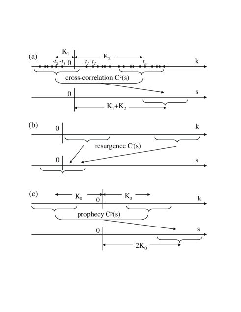
Define the following cross correlation of $\delta\rho_{\epsilon}(k)$ among two windows $[K_{1}-\Delta,K_{1}+\Delta]$ and $[K_{2}-\Delta,K_{2}+\Delta]$ with $K_{1}$, $K_{2}$ any real numbers and $K_{1}\leq K_{2}$ as

$$C_{\rho_{\epsilon}}^{c}(s;K_{1},K_{2},\Delta) \equiv \{\left\langle\delta\rho_{\epsilon}(K_{1}+k)\delta\rho_{\epsilon}(K_{2}+k+s)\right\rangle_{k};\quad|s|\leq\Delta,\text{\ }$$ (3)

$$\quad k\in[-\Delta-\min(0,s),\Delta-\max(0,s)]\}.$$

The superscript “$c$” denotes cross. Here the average over $k$ is defined as

$$\langle f_{1}(k)f_{2}(k)\rangle={\frac{1}{b-a}}\int_{a}^{b}f_{1}(k)f_{2}(k)dk\,.$$

There are two special cases

$$C_{\rho_{\epsilon}}^{r}(s;K_{0},\Delta) \equiv C_{\rho_{\epsilon}}^{c}(s;K_{0},K_{0},\Delta)\equiv\left\langle\delta\rho_{\epsilon}(K_{0}+k)\delta\rho_{\epsilon}(K_{0}+k+s)\right\rangle_{k},$$ (4)

$$C_{\rho_{\epsilon}}^{p}(s;K_{0},\Delta) \equiv C_{\rho_{\epsilon}}^{c}(s;K_{0},-K_{0},\Delta)\equiv\left\langle\delta\rho_{\epsilon}(K_{0}-k)\delta\rho_{\epsilon}(K_{0}+k+s)\right\rangle_{k}.$$ (5)

In Eq. (5), we used $\delta\rho_{\epsilon}(K_{0}-k)=\delta\rho_{\epsilon}(-K_{0}+k)$. The superscript “$r$” and “$p$” denotes resurgence and prophecy, respectively. The meaning will be apparent later.

We now summarize the principal results of this paper. We have the following

CONJECTURE:

1. INVARIANCE the spectral correlation is invariant and independent of averaging window. That is

$$C_{\rho_{\epsilon}}^{c}(s;K_{1},K_{2},\Delta) = C^{\epsilon}(K_{2}-K_{1}+s),$$ (6)

$$C_{\rho_{\epsilon}}^{r}(s;K_{0},\Delta) = C^{\epsilon}(s),$$ (7)

$$C_{\rho_{\epsilon}}^{p}(s;K_{0},\Delta) = C^{\epsilon}(2K_{0}+s)$$ (8)

Note that one has $-\Delta\leq s\leq\Delta$ with $\Delta\gg\,\langle\delta=t_{n}-t_{n-1}\rangle$, the mean spacing between the RZ in a window.

2. The spectral correlation is a sum of functions of the pole and zeros of the Riemann zeta function

$$C^{\epsilon}(s)=\Re\left[g(1+2\epsilon+is,1)-\sum\limits_{n=1}^{\infty}g(1+2\epsilon+is,-2n)-\sum\limits_{n=1}^{\infty}g(1+2\epsilon+is,{\frac{1}{2}}\pm it_{n})\right].$$ (9)

Here $g(z,\alpha)$ is a certain two-variable function. The second (third) term is the summation over trivial (nontrivial) RZ.

3. The function $g(z,\alpha)$ can be broken into diagonal and off-diagonal terms

$$g(z,\alpha)=g_{\text{diag}}(z,\alpha)+g_{\text{off}}(z,\alpha).$$ (10)

Here $g_{\text{off}}\ll$ $g_{\text{diag}}$. Then we show that

$$g_{\text{diag}}(z,\alpha)={\frac{1}{2\pi^{2}}\frac{1}{(z-\alpha)^{2}}-\frac{1}{2\pi^{2}}\sum\limits_{n=2}^{\infty}\frac{c_{n}}{(z-\alpha/n)^{2}}}$$ (11)

with $c_{n}$’s real coefficients, $|c_{n}|\leq 1/n$, and $c_{n}\rightarrow 0$ for $n\rightarrow\infty$. For the correlation function of interest $C_{\rho_{\epsilon}}(s)$ with $s\in[a,b]$, it can be replaced with a finite sum over the pole and zeros of the Riemann zeta function

$$C^{\epsilon}(s)\simeq{\frac{1}{2\pi^{2}}\Re}\left[{\frac{1}{(is+2\epsilon)^{2}}-\sum\limits_{n=1}^{\infty}\frac{1}{(is+{1+}2\epsilon+2n)^{2}}-\sum\limits_{n=N_{0}}^{N}\frac{1}{(is-it_{n}+{\frac{1}{2}+}2\epsilon)^{2}}}\right],$$ (12)

$$s\in[a,b],\quad t_{N_{0}}\lesssim a,\quad t_{N}\gtrsim b.$$

The contribution of RZ far outside $[a,b]$ is small.

4. RESURGENCE

$$C_{\rho_{\epsilon}}^{r}(s;K_{0},\Delta)=C^{\epsilon}(s)\approx-{\frac{1}{2\pi^{2}}}\Re{\sum\limits_{n=1}^{N}\frac{1}{(is\pm it_{n}+{\frac{1}{2}+}2\epsilon)^{2}}},\text{ }|s|<\Delta\text{, }t_{N}\gtrsim\Delta.$$ (13)

5. PROPHECY

$$C_{\rho_{\epsilon}}^{p}(s;K_{0},\Delta)=C^{\epsilon}(2K_{0}+s)\approx-{\frac{1}{2\pi^{2}}}\Re{\sum\limits_{n=N_{0}}^{N}\frac{1}{(is+2iK_{0}-it_{n}+{\frac{1}{2}+}2\epsilon)^{2}}},$$ (14)

$$|s|<\Delta\text{, }t_{N_{0}}\lesssim 2K_{0}-\Delta,\quad t_{N}\gtrsim 2K_{0}+\Delta.$$

A graphic representation of the conjecture is shown in Fig.1.

Figure 1: A sketch of the conjecture: (a) cross-correlation $C_{\rho_{\epsilon}}^{r}(s)$, (b) invariance and resurgence in auto-correlation $C_{\rho_{\epsilon}}^{r}(s)$, (c) prophecy $C_{\rho_{\epsilon}}^{p}(s)$.

A few remarks are in order.

INVARIANCE The invariance of the correlations means that the same structure is encoded in the Riemann spectrum independent of the center and width of the averaging window. The cross correlation $C_{\rho_{\epsilon}}^{c}(s;K_{1},K_{2},\Delta)$ between the spectral function $\delta\rho_{\epsilon}(k)$ in any two windows $[K_{1}-\Delta,K_{1}+\Delta]$ and $[K_{2}-\Delta,K_{2}+\Delta]$ is the same if the center distance $K_{2}-K_{1}$ is the same.

RESURGENCE We find that the peaks of $-C_{\rho_{\epsilon}}^{r}(s)$ are located at the positions $s=t_{n}$. The correlation between RZ in $[K_{0}-\Delta,K_{0}+\Delta]$ leads to RZ in $[-\Delta,\Delta]$. The auto-correlation $C_{\rho_{\epsilon}}^{r}(s)$ in Eq. (4) is essentially the two-level correlation $R_{2}(s)$ Keating96 . Resurgence was first noted by Berry and Keating Berry307 ; Keating ; Connors and has been revisited recently by Leboeuf and collaborators Bohigas01 ; Leboeuf01 ; Leboeuf04 . While the correlations studied in the present paper are related to the above work, the difference is that here, there is no unfolding and no rescaling by the mean level spacing, and reveals some unexpected new results among the RZ summarized in the equations above.

PROPHECY can lead to the prediction of new zeros in the interval $[2K_{0}-\Delta,2K_{0}+\Delta]$ from interval $[K_{0}-\Delta,K_{0}+\Delta]$.

Resurgence and prophecy can also be observed in the cross correlation $C_{\rho_{\epsilon}}^{c}(s;K_{1},K_{2},\Delta)$.

III Trace formula derivation

The above properties are “derived” using a semiclassical method Agam95 . The fluctuation part of the spectral density of the RZ is Berry140 ; Brack

$$\delta\rho_{\epsilon}(k)=-{\frac{1}{\pi}}\sum_{p}L_{p}\sum_{r=1}^{\infty}\Lambda_{p}^{-r({\frac{1}{2}}+\epsilon)}\cos(rkL_{p})$$ (15)

Note that this is exactly of the same form as the Gutzwiller trace formula for chaotic billiards in wave number $k$ Gutzwiller , with length of “periodic orbit” equal to the logarithm of prime numbers $L_{p}=\ln p$ and $\Lambda_{p}=e^{L_{p}}=p$. Like that of the chaotic systems such as the chaotic $n$-disk systems Pance , the number of “periodic orbits” for the RZ grows asymptotically as $N(L_{p}<L)\sim e^{L}/L$. Although the above trace formula converges only for $\epsilon>\frac{1}{2}$, we may still use it formally for $\epsilon\rightarrow 0$. The correlation can be written as the sum of diagonal and off-diagonal terms

$$C_{\rho}^{\epsilon}(s)=\langle\delta\rho_{\epsilon}(k)\delta\rho_{\epsilon}(k+s)\rangle=C_{\text{diag}}^{\epsilon}(s)+C_{\text{off}}^{\epsilon}(s).$$

The diagonal part is

$$C_{\text{diag}}^{\epsilon}(s)={\frac{1}{2\pi^{2}}}\sum_{p}L_{p}^{2}\sum_{r=1}^{\infty}\Lambda_{p}^{-r(1+2\epsilon)}\cos(rsL_{p})=-{\frac{1}{2\pi^{2}}}\Re{\frac{\partial^{2}}{\partial s^{2}}}\sum_{p}\sum_{r=1}^{\infty}{\frac{1}{r^{2}}}t_{p}^{r}$$ (16)

with $t_{p}=\Lambda_{p}^{-(1+2\epsilon)}e^{isL_{p}}=p^{-1-2\epsilon+is}$. $C_{\text{diag}}^{\epsilon}(s)$ can also be broken into two parts Bohigas01 ; Bogomolny03

$$C_{\text{diag}}^{\epsilon}(s)=C_{\mathcal{\zeta}}^{\epsilon}(s)-C_{\mathcal{F}}^{\epsilon}(s)$$ (17)

with

$$C_{\mathcal{\zeta}}^{\epsilon}(s) = -{\frac{1}{2\pi^{2}}}\Re{\frac{\partial^{2}}{\partial s^{2}}}\ln\mathcal{\zeta}(1+2\epsilon+is)$$

$$C_{\mathcal{F}}^{\epsilon}(s) = -{\frac{1}{2\pi^{2}}}\Re{\frac{\partial^{2}}{\partial s^{2}}}\ln\mathcal{F}_{\epsilon}(s).$$ (18)

Here

$$\ln\mathcal{F}_{\epsilon}(s)=\sum_{p}\sum_{r=1}^{\infty}\frac{r}{(r+1)^{2}}t_{p}^{r+1}.$$ (19)

Alternatively, one has the following expressions by direct summation over $r$

$$C_{\text{diag}}^{\epsilon}(s) = {\frac{1}{2\pi^{2}}}\Re\sum_{p}L_{p}^{2}\frac{t_{p}}{1-t_{p}},$$

$$C_{\mathcal{\zeta}}^{\epsilon}(s) = {\frac{1}{2\pi^{2}}}\Re\sum_{p}L_{p}^{2}\frac{t_{p}}{(1-t_{p})^{2}},$$

$$C_{\mathcal{F}}^{\epsilon}(s) = {\frac{1}{2\pi^{2}}}\Re\sum_{p}L_{p}^{2}\frac{t_{p}^{2}}{(1-t_{p})^{2}}.$$ (20)

These expressions have absolute convergence. Obviously, one has $C_{\mathcal{F}}^{\epsilon}(s)<{\frac{1}{2}}C_{\mathcal{\zeta}}^{\epsilon}(s)$.

In order to obtain a compact form for $C_{\mathcal{\zeta}}^{\epsilon}(s)$, we notice the following expression for the Riemann zeta function $\zeta(s)$

$$\mathcal{\zeta}(s)=\frac{e^{(\ln 2\pi-1-\gamma/2)s}}{2(s-1)\Gamma(1+\tfrac{1}{2}s)}\prod_{n}\left(1-\frac{s}{\gamma_{n}}\right)e^{s/\gamma_{n}}$$

with $\gamma_{n}=\frac{1}{2}\pm it_{n}$. One has

$${\frac{\partial^{2}}{\partial s^{2}}}\ln\mathcal{\zeta}(1+is)={\frac{1}{s^{2}}}+\frac{1}{4}\psi_{1}(\tfrac{3}{2}+i\tfrac{1}{2}s){+}\sum_{n}{\frac{1}{(1+is-\gamma_{n})^{2}}.}$$ (21)

Here ${\psi}_{n}(z)\equiv d^{n+1}\Gamma(z)/dz^{n+1}$ is the polygamma function with

$${\psi}_{n}(z)=(-1)^{n+1}n!\sum\limits_{j=0}^{\infty}{\frac{1}{(j+z)^{n+1}}}.$$

Define the following function

$$Z(z)\equiv{\frac{1}{(z-1)^{2}}-\sum\limits_{j=1}^{\infty}\frac{1}{(z+2j)^{2}}-\sum\limits_{j=1}^{\infty}\frac{1}{(z-{\frac{1}{2}}\pm it_{j})^{2}},}$$ (22)

one thus has

$$C_{\mathcal{\zeta}}^{\epsilon}(s)={\frac{1}{2\pi^{2}}\Re}Z(1+2\epsilon+is).$$ (23)

In order to obtain a compact form for the term $C_{\mathcal{F}}^{\epsilon}(s)$, we use the following expansion for small $t$

$$\sum_{q=2}^{\infty}\frac{q-1}{q^{2}}t^{q}=\sum_{n=2}^{\infty}c_{n}\sum_{r=1}^{\infty}\frac{t^{nr}}{r}.$$ (24)

The coefficients ${c_{n}}$ can be obtained by equalizing the coefficients of $t^{q}$ on both sides of the equation. For prime numbers and the power of 2, one has

$$c_{p} = (p-1)/p^{2},$$

$$c_{2^{n}} = 2^{-2n},\text{ }n\geq 1.$$ (25)

The rest of the ${c}_{n}$’s are given by the following recursive equation

$${\sum_{n\geq 2,r\geq 1,nr=q}\frac{1}{r}}c_{n}={\frac{q-1}{q^{2}}.}$$ (26)

For example, one has ${c}_{6}=-1/18$, ${c}_{10}=-1/25$, ${c}_{12}=-1/72$, ${c}_{14}=-3/98$, ${c}_{15}=-8/15^{2}$.

Using the expansion (24) and function $Z(z)$, one has

$$C_{\mathcal{F}}^{\epsilon}(s) = -{\frac{1}{2\pi^{2}}}\Re{\frac{\partial^{2}}{\partial s^{2}}\sum_{n=2}^{\infty}\frac{{c_{n}}}{n^{2}}}\ln\mathcal{\zeta}[n(1+2\epsilon+is)]$$ (27)

$$= {\frac{1}{2\pi^{2}}\Re\sum_{n=2}^{\infty}n^{2}c_{n}}Z[n(1+2\epsilon+is)].$$

One thus gets

$$C_{\text{diag}}^{\epsilon}(s) = -{\frac{1}{2\pi^{2}}\Re\sum_{n=1}^{\infty}n^{2}c_{n}}Z[n(1+2\epsilon+is)]$$ (28)

$$= -{\sum_{n=1}^{\infty}n^{2}c_{n}}C_{\mathcal{\zeta}}^{{\frac{n-1}{2}+n}\epsilon}(ns)$$

with ${c_{1}=-1}$. If one ignores the off-diagonal term $C_{\text{off}}^{\epsilon}(s)$, one obtains (9) with $g(z,\alpha)$ given by Eq. (11).

The value of the correlation at the origin can also be calculated in the following

$$C_{\text{diag}}^{\epsilon}(0)={\frac{1}{2\pi^{2}}}\sum_{p}L_{p}^{2}\sum_{r=1}^{\infty}\Lambda_{p}^{-r(1+2\epsilon)}={\frac{1}{2\pi^{2}}}\sum_{p}{\frac{L_{p}^{2}}{e^{(1+2\epsilon)L_{p}}-1}}.$$

The average density of periodic orbits for large $L$ is $\rho(L)=d(e^{L}/L)dL=(L-1)e^{L}/L^{2}$. Since one has

$$\int_{L}^{\infty}{\frac{L^{2}\rho(L)dL}{e^{(1+2\epsilon)L}-1}}\approx\int_{L}^{\infty}e^{-2\epsilon L}LdL={\frac{1+2\epsilon L}{4\epsilon^{2}}}e^{-2\epsilon L}.$$

Simply set $L=\ln 2$, one has $C_{\text{diag}}^{\epsilon}(0)\approx(1+2\epsilon\ln 2)/8\pi^{2}\epsilon^{2}4^{\epsilon}$. For example for $\epsilon=0.5$, one has $C_{\text{diag}}^{\epsilon}(0)\approx 0.0429$. In the limit $\epsilon\rightarrow 0$, one has $C_{\text{diag}}^{\epsilon}(0)\approx 1/8\pi^{2}\epsilon^{2}$.

IV Numerical results

In order to check the validity of the conjecture, we construct $\delta\rho_{\epsilon}(k)$ according to Eq. (2) from a finite sequence of $t_{n}$ such that $t_{N_{0}}\lesssim K_{0}-\Delta$ and $t_{N}\gtrsim K_{0}+\Delta$. Define $\delta_{N}\equiv 2\pi/\ln(t_{N}/2\pi)$ which is the local level spacing in the neighbourhood of $t_{N}$. We use $\epsilon$ $\sim\delta_{N}$. One has $\delta_{N}\simeq 0.669$, $0.257$, $0.141$, $0.134$ for $N=10^{5}$, $10^{12}$, $10^{21}$, $10^{22}$, respectively. The RZ we studied are obtained from Odlyzko Odlyzko . We find the following properties of spectral correlations of the RZ.

IV.1 Correlation invariance

For the first $10^{5}$ Riemann  zeros, the fluctuation part of the spectral density $\delta\rho_{\epsilon}(k)$ is constructed. We equally divide them into 5 segments : $[K_{n}-\Delta,K_{n}+\Delta]$ with $K_{n}=(2n-1)\Delta+10$, $\Delta=7490$, and $n=1,2,\cdots 5$. Note that $t_{10^{5}}=74920.8$. We then evaluate the auto-correlation $C_{\rho_{\epsilon}}^{r}(s)$ (4) for each segment. We find that without any normalization, all 5 of them collapse to the same curve . As a comparison, we also calculated the auto-correlation for every $2\times 10^{4}$ of the first $10^{5}$ RZ. The correlations are also the same. The relative difference between them is less than 0.1%.

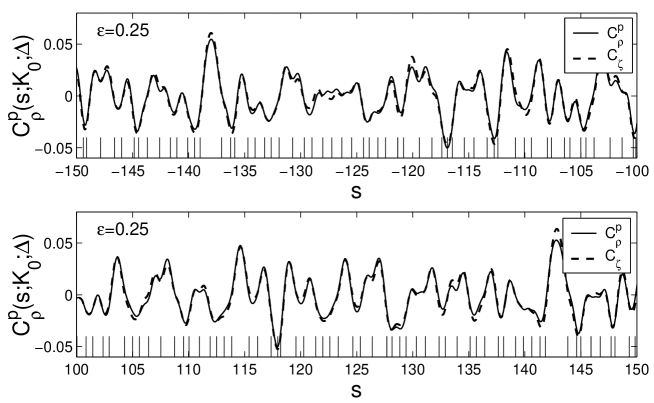
In the same way, we consider four groups of RZ: $\{1,10^{5}\}$, $\{10^{12}+1$, $10^{12}+10^{4}\}$, $\{10^{21}+1,10^{21}+10^{4}\}$, and $\{10^{22}+1$, $10^{22}+10^{4}\}$. For the spectral correlations of the above four segments of RZ with the same width $\epsilon$, they also all collapse to the same curve without any normalization as shown in Fig.2.

Figure 2: Invariance of spectral correlation $C_{\rho}^{r}(s;K_{0};\Delta)$ for RZ with $\epsilon=0.25$: $\{1,10^{5}\}$ (dashed), $\{10^{12}+1,10^{12}+10^{4}\}$ (dash-dotted), $\{10^{21}+1,10^{21}+10^{4}\}$ (dotted), and $\{10^{22}+1,10^{22}+10^{4}\}$ (solid). All curves for different ranges are almost identical.

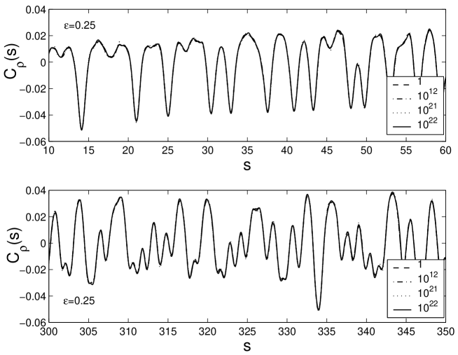
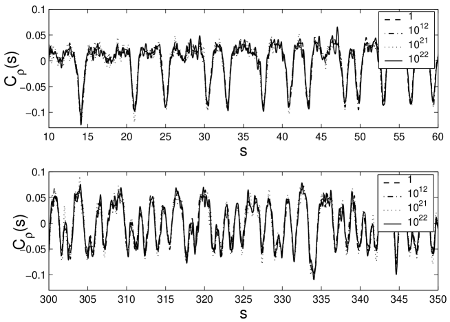
In general, one would expect that the spectral correlation will depend on the choice of $K_{0}$ and $\Delta$ in Eq.(4). Even though the spectrum is more congested around $t_{n}\sim K_{0}$ for larger $n$, they all have almost the same spectral auto-correlation. We find that the main feature of the auto-correlation is only determined by the choice of $\epsilon$ and independent of $K_{0}$ and $\Delta$. So no matter how high the RZ located on the critical line, they are all correlated in the same way as the low lying RZ. The dependence on $K_{0}$ and $\Delta$ will show up for very small width $\epsilon$ such that $\epsilon$ $<\delta$ and very narrow $\Delta$. This is shown in Fig.3 where we used $\epsilon=0.1<\delta_{10^{22}}\simeq 0.134$.

We point out that the diagonal approximation is very accurate for the Riemann  zeros. Numerically calculated $C_{\rho_{\epsilon}}^{r}(s)$ are almost indistinguishable from the direct evaluation of $C_{\text{diag}}(s)$ given in Eq. (20) using the first 350,000 primes for $s<500$. For example for $\epsilon=0.25$, $0.5$, one has the standard deviation $\sigma=\langle C_{\text{off}}^{2}\rangle^{1/2}/\langle C_{\rho}^{r2}\rangle^{1/2}\sim 0.022$, $0.031$, respectively for the spectral correlation of the RZ $\{t_{n}\}$ with $n\sim 10^{12}$.

Figure 3: Same as in Fig.2 with $\epsilon=0.1$.

IV.2 Resurgence

The invariance of the spectral correlations implies the existence of certain intrinsic structure in the spectral auto-correlation. By resurgence of RZ we mean the appearance of RZ $\{{\frac{1}{2}\pm i}t_{n}\}$ with small $n$ from the correlation of RZ with large $n$. We find that the peaks of $-C_{\rho_{\epsilon}}^{r}(s)$ are located at the positions $s=t_{n}$.

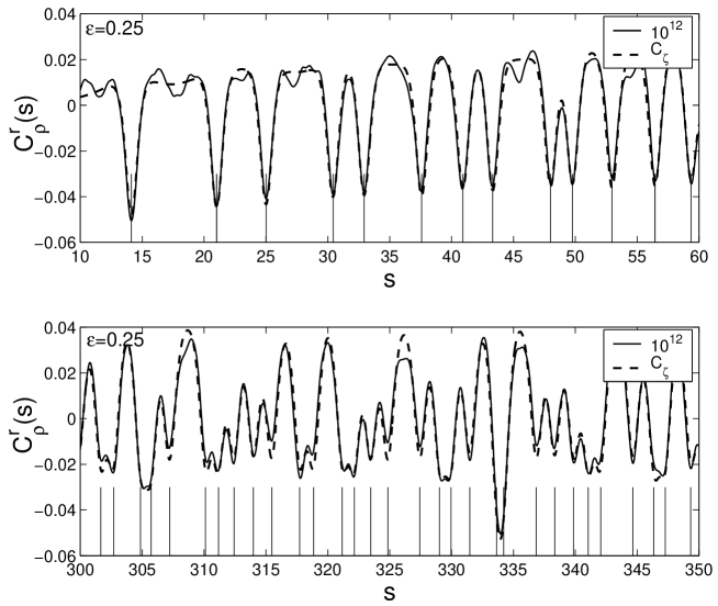
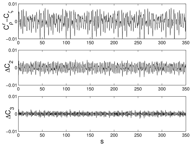
We then use our conjecture (12) to reveal the structure within the auto-correlation. The numerically calculated $C_{\rho_{\epsilon}}^{r}(s;K_{0},\Delta)$ can be approximated very well by $C_{\mathcal{\zeta}}^{\epsilon}(s)$ without any fitting parameters. This is shown in Fig. 4 for width $\epsilon=0.25$. The difference $C_{\rho_{\epsilon}}^{r}(s)-C_{\mathcal{\zeta}}^{\epsilon}(s)$ is very small as shown in Fig. 5a with $\sigma=\langle(C_{\rho_{\epsilon}}^{r}-C_{\mathcal{\zeta}}^{\epsilon})^{2}\rangle^{1/2}/\langle C_{\rho}^{r2}\rangle^{1/2}=0.174,0.155$, for $\epsilon=0.25,0.5$, respectively of the RZ $\{t_{n}\}$ with $n\sim 10^{12}$ for $0<s<350$. Better approximations can be achieved by including more terms in $C_{\text{diag}}^{\epsilon}(s)$. Define the difference of a better approximation according to Eq. (28),

$$\Delta C_{2}(s)=C_{\rho_{\epsilon}}^{r}(s;K_{0},\Delta)-C_{\mathcal{\zeta}}^{\epsilon}(s)+C_{\rho_{\frac{1}{2}+2\epsilon}}^{r}(2s;K_{0},\Delta),$$ (29)

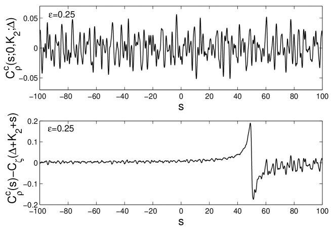
one has the standard deviation reduced to $\sigma=0.093,0.072$, for $\epsilon=0.25,0.5$, respectively. We further define

$$\Delta C_{3}(s)=\Delta C_{2}+2C_{\rho_{1+3\epsilon}}^{r}(3s;K_{0},\Delta),$$ (30)

then the standard deviation $\sigma=0.041,0.036$ for $\epsilon=0.25,0.5$, respectively. This is comparable with the off-diagonal term. The behaviors of $C_{\rho_{\epsilon}}^{r}-C_{\mathcal{\zeta}}^{\epsilon}$, $\Delta C_{2}$, and $\Delta C_{3}$ for $\epsilon=0.25$ are plotted in Fig.5.

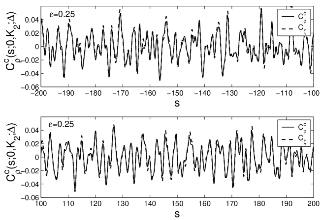
Resurgence can also be observed in the cross correlation $C_{\rho_{\epsilon}}^{c}(s;K_{1},K_{2},\Delta)$ in Eq. (3) for two windows $[K_{1}-\Delta,K_{1}+\Delta]$ and $[K_{2}-\Delta,K_{2}+\Delta]$ with $K_{1}\sim 0$. Suppose we consider the set $\{t_{n}\}$ with $10^{22}<n\leq 10^{22}+10^{4}$. We use $K_{1}=0$, $K_{2}=(t_{10^{22}+1}+t_{10^{22}+10^{4}})/2$, and choose the window size $\Delta=620\sim(t_{10^{22}+10^{4}}-t_{10^{22}+1})/2$ in (3) so that $K_{2}+\Delta\sim t_{10^{22}+10^{4}}$. The spectral function $\delta\rho_{\epsilon}(k)$ is constructed according to Eq. (1) in windows $[-\Delta,\Delta]$ and $[K_{2}-\Delta,K_{2}+\Delta]$. The center distance between these two windows is $K_{2}$. The cross correlation $C_{\rho_{\epsilon}}^{c}(s;0,K_{2},\Delta)$ with $s\in[-\Delta/2,\Delta/2]$ and $\epsilon=0.25$ is shown in Fig.6. One can see that $C_{\rho_{\epsilon}}^{c}(s;0,K_{2},\Delta)$ can be well approximated by $C_{\mathcal{\zeta}}^{\epsilon}(K_{2}+s)$ with $\sigma=\langle(C_{\rho_{\epsilon}}^{c}-C_{\mathcal{\zeta}}^{\epsilon})^{2}\rangle^{1/2}/\langle C_{\rho}^{2}\rangle^{1/2}\sim 0.199,0.171$ for $\epsilon=0.25,0.5$, respectively. To improve the fitting, one can use

$$C_{\rho_{\epsilon}}^{c}(s;0,K_{2},\Delta)\simeq C_{\mathcal{\zeta}}^{\epsilon}(K_{2}+s)-C_{\rho_{{\frac{1}{2}+}2\epsilon}}^{p}(2s;K_{2},\Delta).$$ (31)

Here $C_{\rho_{\epsilon}}^{p}(s;K_{2},\Delta)$ with $-\Delta\leq s\leq\Delta$ is the cross correlation (5) between $[-K_{2}-\Delta,-K_{2}+\Delta]$ and $[K_{2}-\Delta,K_{2}+\Delta]$. This time, the standard deviation is reduced to $\sigma=0.118,0.079$ for $\epsilon=0.25,0.5$, respectively. Similar results are also obtained for $K_{2}\sim t_{10^{12}}$ and $K_{2}\sim t_{10^{21}}$.

Figure 4: Resurgence of RZ in $C_{\rho}^{r}(s;K_{0},\Delta)$ for $\epsilon=0.25$. Here $C_{\rho}^{r}(s;K_{0};\Delta)$ is the numerically calculated auto correlation in $[K_{0}-\Delta,K_{0}+\Delta]$ with $K_{0}=(t_{10^{12}+1}+t_{10^{12}+10^{4}})/2$ and $\Delta\approx(t_{10^{12}+10^{4}}-t_{10^{12}+1})/2$. The dashed curve is $C_{\zeta}^{\epsilon}(s)$. Vertical lines are located at $t_{n}$ and coincide with the valleys.

Figure 5: Resurgence of RZ in $C_{\rho}^{r}(s;K_{0},\Delta)$ for $\epsilon=0.25$. Here $C_{\rho}^{r}(s;K_{0},\Delta)$ is the numerically calculated auto correlation in $[K_{0}-\Delta,K_{0}+\Delta]$ with $K_{0}-\Delta\approx t_{10^{12}+1}$ and $K_{0}+\Delta\approx t_{10^{12}+10^{4}}$. (a) $C_{\rho}^{r}(s;K_{0},\Delta)-C_{\zeta}^{\epsilon}(s)$, (b) $\Delta C_{2}(s)$, (c) $\Delta C_{3}(s)$.

Figure 6: Resurgence of the RZ in the cross correlation $C_{\rho}^{c}(s;0,K_{2},\Delta))$ between $[-\Delta,\Delta]$ and $[K_{2}-\Delta,K_{2}+\Delta]$ with $K_{2}=(t_{10^{22}+1}+t_{10^{22}+10^{4}})/2$ and $\Delta\approx(t_{10^{22}+10^{4}}-t_{10^{22}+1})/2$. The dashed curve is $C_{\zeta}^{\epsilon}(K_{2}+s)$.

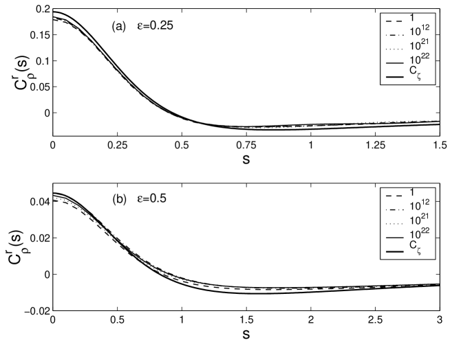
We point out that the small $s$ behavior of $C_{\rho_{\epsilon}}^{r}(s)$ is not a Lorentzian, contrary to the claim in Wardlaw . According to (12), one has

$$C_{\rho_{\epsilon}}^{r}(s)\simeq(4\epsilon^{2}-s^{2})/2\pi^{2}(s^{2}+4\epsilon^{2})^{2}$$ (32)

for $s\leq 5$. So that $C_{\rho_{\epsilon}}^{r}(0)\simeq 1/(8\pi^{2}\epsilon^{2})$. This value is very close to that at the origin for different auto-correlations. The behavior of $C_{\rho_{\epsilon}}^{r}(s)$ for small $s$ is shown in Fig.7 for different segments of RZ.

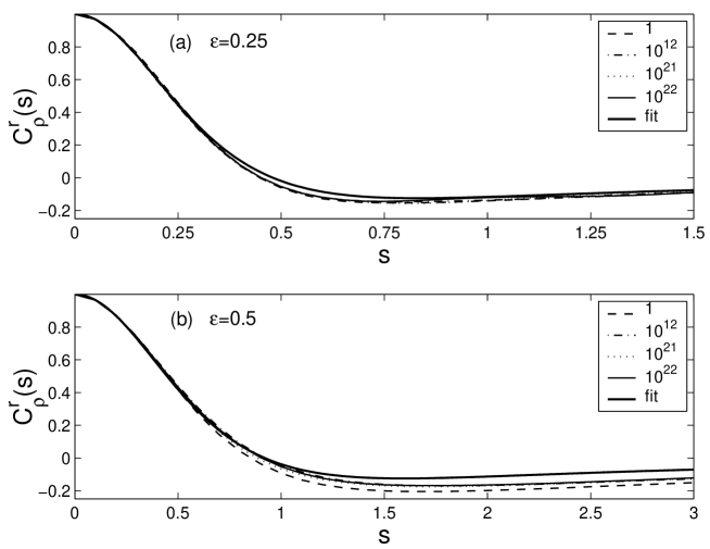
The ratio $C_{\rho_{\epsilon}}^{r}(s)/C_{\rho_{\epsilon}}^{r}(0)$ can be very well fitted by

$$C_{\rho_{\epsilon}}^{r}(s)/C_{\rho_{\epsilon}}^{r}(0)=4\beta^{2}(4\beta^{2}-s^{2})/(s^{2}+4\beta^{2})^{2}$$ (33)

with fitting parameter $\beta\sim\epsilon$ for small $s$. This is shown in Fig.8. As we mentioned before, $\delta\rho_{\epsilon}(k)$ is related to the fluctuation part of the time delay $\tau_{\text{fl}}(w)$, so $C_{\rho_{\epsilon}}^{r}(s)$ is related to the auto-correlation of the time delay $c(\varepsilon;w_{c},\Delta)$ discussed in Wardlaw with $\epsilon=0.5$ and $s=2\varepsilon$. Thus for small $\varepsilon$, $c(\varepsilon;w_{c},\Delta)$ can be better fitted by Eq. (32) with $\beta=0.46$ as shown in Fig.8b.

Figure 7: Small $s$ behavior of $C_{\rho}^{r}(s)$ with (a) $\epsilon=0.25$ and (b) $\epsilon=0.5$ for RZ: $\{1,10^{5}\}$ (dashed), $\{10^{12}+1,10^{12}+10^{4}\}$ (dash-dotted), $\{10^{21}+1,10^{21}+10^{4}\}$ (dotted), and $\{10^{22}+1,10^{22}+10^{4}\}$ (solid). The bold solid line is $C_{\zeta}(s)$ (Eq.(12)).

Figure 8: Small $s$ behavior of $C_{\rho}^{r}(s)/C_{\rho}^{r}(0)$ with (a) $\epsilon=0.25$, $\beta=0.24$ and (b) $\epsilon=0.5$ , $\beta=0.46$ for RZ: $\{1,10^{5}\}$ (dashed), $\{10^{12}+1,10^{12}+10^{4}\}$ (dash-dotted), $\{10^{21}+1,10^{21}+10^{4}\}$ (dotted), and $\{10^{22}+1,10^{22}+10^{4}\}$ (solid). Here $\beta$ is the fitting parameter in Eq. (33).

IV.3 Prophecy

By prophecy of RZ we mean the appearance of RZ $\{{\frac{1}{2}\pm i}t_{n}\}$ with large $n$ from the correlation of RZ with small $n$. We consider the correlation $C_{\rho_{\epsilon}}^{p}(s;K_{0},\Delta)$ in Eq. (5) for RZ $\{1,10^{4}\}$. The prophecy of new RZ from $C_{\rho_{\epsilon}}^{p}(s;K_{2},\Delta)$ with $\epsilon=0.25$ is shown in Fig.9. The agreement with Eq.(14) is very good.

Prophecy can also be observed in the cross correlation $C_{\rho_{\epsilon}}^{c}(s;K_{1},K_{2},\Delta)$ in Eq. (3) for two windows $[K_{1}-\Delta,K_{1}+\Delta]$ and $[K_{2}-\Delta,K_{2}+\Delta]$ with $K_{1}+\Delta\sim 0$. As in the above subsection, we consider the set $\{t_{n}\}$ with $10^{22}<n\leq 10^{22}+10^{4}$. We use $K_{1}=-\Delta$, $K_{2}=(t_{10^{22}+1}+t_{10^{22}+10^{4}})/2$, and choose the window size $\Delta=(t_{10^{22}+10^{4}}-t_{10^{22}+1})/2-50=620.8$. $\delta\rho_{\epsilon}(k)$ is calculated in windows $[-2\Delta,0]$ and $[K_{2}-\Delta,K_{2}+\Delta]$. The center distance between these two windows is $K_{2}+\Delta\approx t_{10^{22}+10^{4}}$. The cross correlation $C_{\rho_{\epsilon}}^{c}(s;\Delta,K_{2},\Delta)$ is shown in Fig.10. If $s\leq 50$, one has resurgence of RZ since $s+\Delta+K_{2}\leq t_{10^{22}+10^{4}}$. If $s>50$, one has prophecy of new RZ. Similar results are also obtained for $K_{2}\sim t_{10^{12}}$ and $K_{2}\sim t_{10^{21}}$.

Figure 9: Prophecy of the RZ in $C_{\rho_{\epsilon}}^{p}(s;K_{0},\Delta)$ for RZ $\{1,10^{4}\}$ with $\epsilon=0.25$, $K_{0}=4941.4$ , and $\Delta=4920$. The dashed curve is $C_{\zeta}^{\epsilon}(2K_{0}+s)$. The vertical lines are at $s=t_{n}-2K_{0}$.

The above long range correlation can be used to calculate RZ from known ones. When applied to prophecy correlation $C_{\rho_{\epsilon}}^{p}(s)$, new RZ can be obtained. The Fourier transformation of $C_{\rho_{\epsilon}}(s)$ is

$$\widetilde{C}(x)=\int C_{\rho_{\epsilon}}(s)e^{isx}ds\simeq-{\frac{1}{2\pi}x}\sum_{n}e^{it_{n}x-\gamma x}$$ (34)

with $\gamma=1+2\epsilon$. $\widetilde{C}(x)$ will have peaks at $x=rL_{p}$. Since the above expression is a sum over different exponentially decaying modes, one may use the Prony algorithm to get $t_{n}$. The above method provides a way to calculate or at least to estimate new RZ.

Figure 10: Prophecy of the RZ in the cross correlation $C_{\rho_{\epsilon}}^{c}(s;\Delta,K_{2},\Delta)$ between $[-2\Delta,0]$ and $[K_{2}-\Delta,K_{2}+\Delta]$ for $\epsilon=0.25$. (a) $C_{\rho_{\epsilon}}^{c}(s;\Delta,K_{2},\Delta)$, (b) $C_{\rho_{\epsilon}}^{c}(s;\Delta,K_{2},\Delta)-C_{\zeta}^{\epsilon}(s+\Delta+K_{2})$. Here $C_{\zeta}^{\epsilon}(s+\Delta+K_{2})$ is calculated from Eq. (12) with $t_{n}$ only up to $N=10^{22}+10^{4}$.

V Discussion: Self-Duality of the Riemann spectrum

The motivation for this work has come from experimental observations in the microwave transmission of open $n$-disk billiards which led to the observation of classical Ruelle-Pollicott (RP) resonances in the auto-correlation of quantum spectra of hyperbolic $n$-disk open billiards Pance . The result established a new approach to quantum-classical correspondence by demonstrating a correspondence between the quantum and classical resonance spectra of an open chaotic system. Applying the same procedures developed there to the Riemann spectrum, we have arrived at the results described in this paper. There are other parallels which are summarized below.

1. In $n$-disk open billiards mentioned above Pance , the experimental trace was fitted well by the sum of Lorentzians $T(k)=\sum_{n}b_{n}/[(k-k_{n})^{2}+k_{n}^{\prime 2}]$. Here $\{k_{n}+ik_{n}^{\prime}\}$ is the spectrum of eigen-wave vector resonances, which are eigenvalues of the Helmholtz (or Laplace-Beltrami) operator, with Dirichlet boundary conditions $(\nabla^{2}+k^{2})\psi=0$, $\psi=0$ on $\partial D.$ We showed that the auto-correlation of the transmission $C(\kappa)=\left\langle T(k)T(k+\kappa)\right\rangle$ are well-described as a sum of Lorentzians $C(\kappa)=\sum_{i}c_{i}/[(\kappa-\gamma_{i}^{{}^{\prime}})^{2}+\gamma_{i}^{\prime\prime 2}]$. Here $\gamma_{i}^{{}^{\prime}}+i\gamma_{i}^{\prime\prime}$are the classical RP resonances. The coefficients $c_{i}$ are related to the eigen-functions of the Perron-Frobenius operator. The $c_{i}$ are all positive, whereas the coefficients are negative for the RZ. For hyperbolic systems, Ruelle has related these eigenvalues to the time-evolution of classical correlations Ruelle86 . The above result can be viewed in the context of dynamic Ruelle zeta functions which are relevant to the $n$-disk billiard. The semiclassical Ruelle zeta-function is $\zeta_{j}(-ik)=\prod_{p}\left[1-e^{i(kL_{p}+\pi\mu_{p}/2)}/\sqrt{\left|\Lambda_{p}\right|}\Lambda_{p}^{j-1}\right]^{-1}$whose poles are the quantum resonances $\{k_{n}+ik_{n}^{\prime}\}$, while the poles of the classical Ruelle zeta-function $\zeta_{\beta}(s)=\prod_{p}\left(1-e^{-sL_{p}}/\Lambda_{p}^{\beta}\right)^{-1}$ are the classical resonances $\{\gamma^{\prime}+i\gamma^{\prime\prime}\}$ CvitanovicBook ; Gaspard . The product is over all classical primitive periodic orbits without repetition. Here $L_{p}$ is the length of periodic orbits with the Maslov index $\mu_{p}$. $\Lambda_{p}$ is the bigger eigenvalue of the Monodromy stability matrix for billiard systems. Mathematically the quantum-classical correspondence can be viewed as a duality between the poles of the semi-classical and classical dynamic zeta functions through the auto-correlation procedure, i.e. $C\{k_{n}+ik_{n}^{\prime}\}\Rightarrow$ $\{\gamma_{i}^{{}^{\prime}}+i\gamma_{i}^{\prime\prime}\}$.

2. For the two-disk billiard (i.e. $n=2$), the semiclassical resonances in wave vector space are $k_{n}=[n\pi+i(1/2)\ln\Lambda]/(R-2a)$ with $\Lambda=\sigma-1+\sqrt{\sigma(\sigma-2)}$ the eigenvalue of the instability matrix in the fundamental domain and $\sigma=R/a$. Here $n$ is odd for $A_{1}$ representation, $n$ even and $n\neq 0$ for $A_{2}$ representation Wirzba92 . The classical RP resonances of the two-disk system are $\gamma_{n}=[\ln\Lambda+in\pi]/(R-2a)$. In this case there is a direct 1-to-1 correspondence between quantum and classical resonances.

3. In the cases of the rectangle billiard and the equal-lateral triangle billiard, the auto-correlation $C_{\rho_{\epsilon}}^{r}(s)$ are shown Lu2004a to correspond to the Fourier transform of the trace of the classical evolution operator, i.e.

   $$C_{\rho_{\epsilon}}(s)\simeq F\Big{[}\mathrm{tr}\mathcal{L}^{t}=\sum_{p}\sum_{r=1}^{\infty}\frac{a_{p}}{rL_{p}}\delta(l-rL_{p})\Big{]}=\sum_{p}\sum_{r=1}^{\infty}\frac{a_{p}}{rL_{p}}\cos(rsL_{p}).$$

   There again the property of correlation invariance and resurgence are clearly demonstrated.

4. For a particle on a surface of constant negative curvature, a self-duality exists for the quantum momentum spectrum, $\{p_{n}\}$ and the classical spectrum $\{\gamma_{n}=\frac{1}{2}\pm ip_{n}\}$ Biswas . The quantum eigen-energy are given by $E_{n}=\frac{1}{4}+p_{n}^{2}$.

Motivated by these observations, we examine a dynamic interpretation of the Riemann zeta function. One has the following expression due to Riemann Riemanntrace

$$\sum\limits_{p}\sum_{r}{\frac{1}{r}}\delta(x-p^{r})=\frac{{1}}{{\ln x}}{-\frac{1}{x(x^{2}-1)\ln x}-2}\sum_{n}{\frac{\cos\left(t_{n}\ln x\right)}{x^{{\frac{1}{2}}}\ln x}}$$ (35)

where $x>1$. Define $l=\ln x$, multiple $\ln x$ to both sides, one has

$$\sum\limits_{p}\sum_{r}{\frac{\ln p}{p^{r}}\delta(l-r\ln p})=1-{\frac{e^{-2l}}{2\sinh l}-}\sum_{n}e^{-({\frac{1}{2}\pm i}t_{n})l}$$ (36)

which is valid for $l>0$. Note the analog with the classical trace formula Cvitanovic ,

$$\text{tr}\mathcal{L}^{t}=\sum\limits_{p}\sum_{r}{\frac{L_{p}}{\Lambda_{p}^{r}}\delta(l-r}L_{p})$$

with $l=t\sqrt{E}$. Thus one has formally

$$\text{tr}\mathcal{L}^{t}=1+\sum_{n}g_{n}e^{-\gamma_{n}l}=1-\sum_{n=1}^{\infty}e^{-({2n+1})l}-\sum_{n=1}^{\infty}e^{-({\frac{1}{2}\pm i}t_{n})l}.$$ (37)

This is very similar to the case for the motion on the surface of constant negative curvature, where the quantum eigen-momentum spectrum is $\{p_{n}\}$. There tr$\mathcal{L}^{t}=1+\sum_{n=1}^{\infty}e^{-({\frac{1}{2}\pm i}p_{n})l}$. Furthermore Biswas and Sinha have shown that the classical resonances are given by $\gamma_{n}=\frac{1}{2}\pm ip_{n}$ Biswas by demonstrating that the peaks of the power spectrum of classical correlations indeed coincide with $\{p_{n}\}$.

For the RZ, the result of performing the auto-correlation of the smoothed density of states then leads to a self-dual “classical” spectrum $\{\frac{1}{2}\pm it_{n}\}$. So one might say that the classical resonances are $\gamma_{n}={\frac{1}{2}\pm i}t_{n}$. This interpretation of RZ as RP resonances was suggested recently Bohigas01 ; Leboeuf04 . However here $g_{n}=-1$ for the RZ while $g_{n}=1$ for the Riemann zeta function pole and RP resonances. This is related to the well-known sign problem for which a possible explanation has been offered by Connes Connes . .

We have clearly established a self-duality which then strongly suggests the interpretation of the spectrum $\{t_{n}\}$ as momentum or wave vector eigenvalues of a Helmholtz operator on a suitable domain. A similar description has been made in which the Riemann zeta function appears in the scattering matrix of the quantum scattering of a particle on a 2D surface of constant negative curvature Wardlaw ; levay , so that $\{{1\over 2}t_{n}\}$ are the real parts of the poles of the scattering matrix.

VI Conclusion

In this paper, we report the observation of new correlations among the RZ that presented as a conjecture supported by analytical arguments and numerical simulations. The spectral correlations possess three important properties: invariance, resurgence and prophecy. The prophecy can be used to progressively obtain new RZ from known ones. The last observation suggests an interesting new strategy for proving the Riemann hypothesis via a bootstrap approach starting with known zeros.

We thank F.Y. Wu and J.V. José for discussions. This work is supported partially by NSF-PHY-0098801.

^†w.lu@neu.edu ^∗s.sridhar@neu.edu

References

- (1) Conrey J B 2003 Notices of the AMS 50, 341.
- (2) Edwards H M 1974 Riemann’s Zeta Function (Academic Press, New York).
- (3) Titchmarsh E C 1986 The Theory of the Riemann Zeta-function, Oxford Science publications, 2nd ed., revised by D.R. Heath-Brown.
- (4) Berry M V 1985 Proc. Roy. Soc. Lond 400, 229.
- (5) Berry M V 1988 Nonlinearity 1, 399.
- (6) Keating J P and Bogomolny E B 1996 Phys. Rev. Lett. 77, 1472.
- (7) Keating J P 1999 in Supersymmetry and Trace Formulae: Chaos and Disorder, eds. Lerner I V, Keating J P, and Khmelnitskii D E (Plenum Press), p.1.
- (8) Berry M V and Keating J P 1999 in Ref. Keating , p.355.
- (9) Berry M V and Keating J P 1999 SIAM Review 41, 236.
- (10) Connors R D and Keating J P 2001 Found. Phys. 31, 669.
- (11) Odlyzko A M 2001 in Dynamical, Spectral, and Arithmetic Zeta Functions, eds. van Frankenhuysen M and Lapidus M L, AMS Contemporary Math. series 290, p.139.
- (12) Bohigas O, Leboeuf P, and Sanchez M J 2001 Found. Phys. 31, 489.
- (13) Leboeuf P, Monastra A G, and Bohigas O 2001 Regular and Chaotic Dynamics 6, 205.
- (14) Leboeuf P 2004 Phys. Rev. E 69, 026204.
- (15) van Zyl B P and Hutchinson D A W 2003 Phys. Rev. E 67, 066211.
- (16) Sakhr J, Bhaduri R K , and van Zyl B P 2003 Phys. Rev. E 68, 026206.
- (17) Bogomolny E B 2003 arXiv: nlin.CD/0312061.
- (18) Sabbagh K 2003 The Riemann Hypothesis: The Greatest Unsolved Problem in Mathematics (Farrar Straus & Giroux, 2003).
- (19) Wu H and Sprung D W L 1993 Phys. Rev. E 48, 2595; Ramani A, Grammaticos B, and Caurier E 1995 Phys. Rev. E 51, 6323.
- (20) Rosu H C 2003 Mod. Phys. Lett. A 18, 1205.
- (21) Katz N M and Sarnak P 1999 Bull. Amer. Math. Soc. 36, 1.
- (22) Berry M V 1986 in Quantum chaos and statistical nuclear physics, eds. T.H. Seligman and H. Nishioka, Springer Lecture Notes in Physics No. 263, p.1.
- (23) Montgomery H L 1973 Proc. Symp. Pure Math. 24, 181.
- (24) Pance K, Lu W, and Sridhar S 2000 Phys. Rev. Lett. 85, 2737; Lu W T, Pance K, Pradhan P, and Sridhar S 2001, Phys. Scrip. T90, 238.
- (25) Brack M and Bhaduri R K 1997 Semiclassical Physics (Addison-Wesley Publishing Company, Inc.), ch.7.
- (26) Wardlaw D M and Jaworski W 1989 J. Phys. A 22, 3561.
- (27) Gutzwiller M C, Chaos in classical and quantum mechanics (Springer-Verlag, 1990).
- (28) Agam O, Altshuler B L, and Andreev A V 1995 Phys. Rev. Lett. 75, 4389.
- (29) Levay P 2000 J. Phys. A 33, 4129.
- (30) Odlyzko A M, http://www.dtc.umn.edu/~odlyzko/zeta_tables/.
- (31) Ruelle D 1986 Phys. Rev. Lett. 56, 405.
- (32) Cvitanović P, Artuso R, Mainieri R, and Vattay G, Classical and Quantum Chaos: a Cyclist Treatise (http://www.nbi.dk/ChaosBook/).
- (33) Gaspard G 1998 Chaos, Scattering and Statistical Mechanics (Cambridge University Press, Cambridge, U.K.).
- (34) Wirzba A 1992 Chaos 2, 77.
- (35) Lu W T, Zeng W, and Sridhar S (to be published).
- (36) Biswas D and Sinha S 1993 Phys. Rev. Lett. 71, 3790.
- (37) Riemann B 1859 Monatsber. Akad. Berlin, 671. The English translation can be found in the appendix of Ref.Edwards . See also Ref.Sakhr03 .
- (38) Cvitanović P and Eckhardt B 1991 J. Phys. A 24, L237.
- (39) Connes A 1999 Sel. Math. New Ser. 5, 29.