A Numerical Study of a Simple Stochastic/Deterministic Model of Cycle-to-Cycle Combustion Fluctuations in Spark Ignition Engines

G. LITAK
Department of Applied Mechanics, Technical University of Lublin, Nabystrzycka 36,
PL-20-618 Lublin, Poland

M. WENDEKER
M. KRUPA
Department of Internal Combustion Engines, Technical University of Lublin,
Nabystrzycka 36, PL-20-618 Lublin, Poland

J. CZARNIGOWSKI
Department of Machine Construction, Technical University of Lublin, Nabystrzycka 36, PL-20-618 Lublin, Poland

We examine a simple, fuel-air, model of combustion in spark ignition (si) engine with indirect injection. In our two fluid model, variations of fuel mass burned in cycle sequences appear due to stochastic fluctuations of a fuel feed amount. We have shown that a small amplitude of these fluctuations affects considerably the stability of a combustion process strongly depending on the quality of air-fuel mixture. The largest influence was found in the limit of a lean combustion. The possible effect of nonlinearities in the combustion process has been also discussed.

Key Words: stochastic noise, combustion, engine control

1 Introduction

Cyclic combustion variability, found in 19th century by Clerk (1886) in all spark ignition (si) engines, has attracted a great interest of researchers during last years (Heywood 1988, Daily 1988, Foakes et al. 1993, Chew et al. 1994, Hu 1996, Daw et al. 1996, 1998, 2000, Letellier et al. 1997, Green Jr. et al. 1999, Rocha-Martinez et al. 2002, Wendeker et al. 2003, 2004, Kamiński et al. 2004). Its elimination would give 10% increase in the power output of the engine. The main sources of cyclic variability were classified by Heywood (1988) as the aerodynamics in the cylinder during combustion, the amount of fuel, air and recycled exhaust gases supplied to the cylinder and a mixture composition near the spark plug.

The key source of their existence may be associated with either stochastic disturbances (Roberts et al. 1997, Wendeker et al. 2000) or nonlinear dynamics (Daw et al 1996, 1998) of the combustion process. Daw et al. (1996, 1998) and more recently Wendeker et al. (2003, 2004) have done the nonlinear analysis of the experimental data of such a process.

Various attempts have been done to explain this phenomenon Shen et al. (1996) modelled a kernel and a front of flame in the cylinder. Their motions and interactions with cylinder chamber walls influenced the region of combustion leading to turbulent behaviour. Hu (1996) developed a phenomenological combustion model and examined the system answer on small variations of different combustion parameters as changes in fuel-air mixture. Stochastic models of internal combustion basing on residual gases where considered by Daw et al. (1996, 1998, 2000), Roberts et al. (1997), Green Jr. et al. (1999), and recently by Rocha-Martinez et al. (2002), who examined multi-input combustion models. Daw and collaborators described the combustion process using a recurrence model with nonlinear combustion efficiency and invented symbolic analysis for combustion stability.

In this paper follow these investigations with a new model assuming that variations of a fresh fuel amount is the most common source of instability in indirect injection.

The present paper is organised as follows. After the introduction in the present section we define the model by a set of difference equations in the next section (Sec. 2). This model, in deterministic and stochastic forms, will be applied in Sec. 3, where we analyse the oscillations of burned mass. Finally we derive conclusions and remarks in Sec. 4.

2 Two fluid model of fuel-air mixture combustion

Starting from fuel-air mixture we define the time evolution of the corresponding amounts. Namely, we will follow the time histories of the masses of fuel $m_{f}$, and air $m_{a}$.

Table 1: Constants and variables of the model.

stoichiometric coefficient	$1/s=14.63$
residual gas fraction	$\alpha=0.08$, 0.16
air mass in a cylinder	$m_{a}$
fuel mass in a cylinder	$m_{f}$
fresh air amount	$\delta m_{a}$
fresh fuel amount	$\delta m_{f}$
air/fuel ratio	$r=m_{a}/m_{f}$
burned fuel mass	$\Delta m_{f}$
combusted air mass	$\Delta m_{a}$
air/fuel equivalence ratio	$\lambda$
random number generator	$N(0,1,i)$
mean value
of fresh fuel amount	$\delta m_{fo}$
standard deviation
of fresh fuel amount	$\gamma=\sigma_{mf}$
standard deviation
of the equivalence ratio	$\sigma_{\lambda}$

Figure 1: The combustion curve $\Delta m(\lambda)$ for the constant fresh air feed $\delta m_{a}=200$ mg.

Firstly, we assume the initial value of $m_{a}(i)$, $m_{f}(i)$ and automatically their ratio $r(i)$:

$$r(i)=\frac{m_{a}(i)}{m_{f}(i)}$$ (1)

for $i=0$.

Secondly, depending on parameter $r$ with reference to a stoichiometric constant $s$ we have two possible cases: fuel and air deficit, respectively. For a deterministic model, the first case lead to

$$r(i)>1/s$$ (2)

we calculate next masses using following difference equations:

$$m_{f}(i+1) = \alpha\left(m_{f}(i)-\frac{1}{s}m_{a}(i)\right)+\delta m_{f}$$

$$m_{a}(i+1) = \delta m_{f},$$ (3)

where $\alpha$ is the residual gas fraction of the engine, $\delta m_{f}$ and $\delta m_{a}$ denotes fresh fuel and air amounts added in each combustion cycle $i$. In the opposite (to Eq. 2) case

$$r(i)<1/s$$ (4)

we use the different formula

$$m_{f}(i+1) = \delta m_{f}$$

$$m_{a}(i+1) = \alpha\left(m_{a}(i)-sm_{f}(i)\right)+\delta m_{a}$$ (5)

Note that variables $m_{a}$ and $m_{f}$ are the minimal set of our interest. From the above equations one can easily calculate other interesting quantities as the combusted masses of fuel $\Delta m_{f}(i)$ and air $\Delta m_{a}(i)$ and air-fuel equivalence ratio before each combustion event $i$:

$$\lambda\approx s\frac{m_{a}(i)+\alpha\Delta m_{a}(i-1)}{m_{f}(i)+\alpha\Delta m_{f}(i-1)}$$ (6)

Basing on experimental results we use the additional necessary condition (Kowalewicz 1984) of combustion process

$$0.6<\lambda<1.3.$$ (7)

For better clarity our notations of system parameters: constants and variables are summarised in Tab. 1.

Basing on the relations (Eqs. 1-7) we plotted the combustion curve for the assumed constant fresh air feed $\delta m_{a}=200$ mg. This value will be used for all simulations throughout this paper.

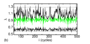
Figure 2: The dependence of $\lambda$ on sequential cycles $i$ for deterministic (a) and stochastic (b) processes. The fresh air amount was assumed to be $\delta m_{a}=200$ mg while the fresh fuel amount varies: $\delta m_{f}=13.50$ mg , 14.63 mg, 21.00 mg starting from the top curve, respectively.

Finally, in the case of stochastic injection, instead of constant $\delta m_{f}(i)$ (Eqs. 3 and 5) (for each cycle $i$) we introduce its mean value $\delta m_{fo}={\rm const.}$, while $\delta m_{f}$ in the following way:

$$\delta m_{f}(i)=\delta m_{fo}+\gamma N(0,1,i),$$ (8)

where $N(0,1,i)$ represents random number generator giving a sequence $i$ of numbers with a unit-standard deviation of normal (Gaussian) distribution and the nodal mean. The scaling factor $\gamma=\sigma_{mf}$ corresponds to the mean standard deviation of the fuel injection amount. The cyclic variation of $\delta m_{f}(i)$ can be associated with such phenomena as fuel vaporisation and fuel-injector variations.

3 Oscillations of burned fuel mass

Here we describe the results of simulations. Using Eqs. 1-8 we have performed recursive calculations for deterministic and stochastic conditions and obtained time histories of various system parameters: $m_{f}$, $m_{a}$, $\Delta m_{f}$, $\Delta m_{a}$ and $\lambda$. The results for $\lambda$ are shown in Fig. 2. The upper panel (Fig. 2a), corresponding to deterministic combustion for three different values of fuel injection parameter $\delta m_{f}$, shows $\lambda$ as straight lines versus cycle $i$, while the lower (Fig. 2b) one reflects the variations of $\lambda$ in stochastic conditions. The order of curves appearing in the Fig. 2b is the same as in Fig. 2a stating from the smallest value of considered fuel injection amounts from the top. To get a more clear insight of random fuel injection on the engine dynamics , in our stochastic simulations, we assumed standard deviation of its mean value $\gamma=\sigma_{mf}=0.1~{}\delta m_{fo}$ to be high enough. In following calculations it was equal to 10%. The obtained results clearly indicate that the fluctuations of $\lambda$ are growing with larger $\lambda$. This can be also found by analytical evaluation of Eq. 6. It is not difficult to check that

$$\sigma_{\lambda}\sim\lambda^{2}\sigma_{mf}.$$ (9)

Figure 3: The dependence of burned fuel mass on sequential cycles $i$ for deterministic (a) and stochastic (b-d) processes. $\delta m_{a}=200$ mg while $\delta m_{f}$ takes different values: 13.50 mg , 14.63 mg, 21.00 mg denoted in particular figures.

The results for burned fuel mass $\Delta m_{f}$ are presented in Fig. 3. Starting from deterministic conditions ($\delta m_{f}=\delta m_{fo}={\rm const.}$) we obtain the constant fraction of the burned fuel mass $\Delta m_{f}$ represented by the three straight lines in Fig. 3a. All lines are lying very close to each other and they are hardly distinguishable in Fig. 3a, but actual numbers shows clearly that $\Delta m_{f}$ increases slightly with growing $\delta m_{f}$ ($\Delta m_{f}=13.50$ mg for $\delta m_{f}=13.50$ mg while $\Delta m_{f}=13.67$ mg for $\delta m_{f}=14.63$ mg and 21.00 mg) account for combustion constraints (Eqs. 1-7) and combustion curve (Fig. 1).

In Fig 3 b-c we show the same, $\Delta m_{f}$, for the considered case of assumed fuel injection ($\delta m_{fo}=13.50$ mg - Fig. 3b, $\delta m_{fo}=14.63$ mg - Fig. 3c, $\delta m_{fo}=21.00$ mg - Fig. 3d) and stochastic conditions. Due to different magnitudes parameter $\lambda$ fluctuations, and dependence of combustion curve Fig. 1 it is not surprise that the fluctuations of $\Delta m_{f}$ have different character in all these cases. For lean combustion, which is a stable process in deterministic case, the fuel injection fluctuations introduce considerable instabilities to the combustion process leading to the suppression of combustion because in some cycles (Fig. 3b) where $\lambda$ is larger that $1.3$.

Figure 4: Return maps for burned fuel mass: $m_{i}(i+1)$ versus $m_{i}(i)$, where $i$ denotes a present cycle for stochastic process ($\gamma=10\%$). $\delta m_{a}=200$ mg while $\delta m_{f}$ takes different values: 13.50 mg , 14.63 mg, 21.00 mg denoted in particular figures. Note, arrows in Figs. 4c and f indicate singular points on return maps for $\delta m_{f}$=21.00 mg.

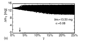
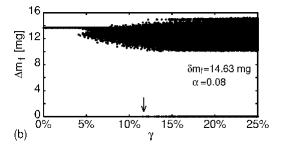
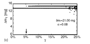
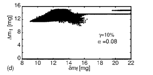
Figure 5: Bifurcation diagrams. $\delta m_{f}$ against noise (Fig. 5a-c) and against the fresh fuel amount constant $\delta m_{f}$ for $\alpha=0.08$. Arrows indicate a bifurcation regarding to misfires appearance.

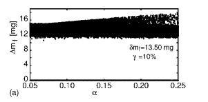
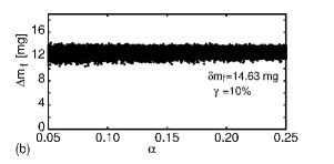
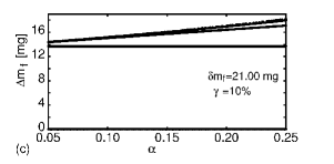
Figure 6: Bifurcation diagrams: $\Delta m_{f}$ against a residual gas fraction $\alpha$ for various fresh fuel amounts $\delta m_{f}$.

Then Equation 7 is not satisfied. In the next case (Fig. 3c) the effect of stochasticity is much smaller. Here we have optimal air-fuel mixture. First of all one should note that fluctuations of $\lambda$ are smaller than in previous case (Fig. 2b). Moreover $\lambda$ oscillate around the region ($\lambda\approx 1$) in combustion curve (Fig. 1) which does not have big changes comparing to previous case. Finally, Fig. 3d shows the sequence of $\Delta m_{f}$ for the large $\delta m_{fo}$ (rich fuel-air mixture). The fluctuations of $\lambda$ are the smallest of all three ones but $\lambda\approx 0.7$ causes suppressions of combustions in some cycles similarly to the case shown in Fig. 3b.

In Figs. 4a-c we have plotted return maps of all considered stochastic cases Figs. 3b-d. Additionally, we have shown similar plots for higher residual gas fraction $\alpha=0.16$ (Figs. 4d-f). Note that differences between both cases ($\alpha$ =0.08 and 0.16) are small. It is also worth to note this results are agreement with diagrams of experimental heat release data for engines Kohler and Quad4 presented by Green Jr. and coworkers (Fig. 1 in Green et al. 1999) for three values of an equivalence ration. Of course heat release can be treated, in the first approximation, as proportional to burned mass through a heating constant of fuel. The only important difference visible between our simulated and experimental data is that the second is more smeared. This could be connected with our model assumptions basing on two components. In reality there are more components (Heywood 1988, Rocha-Martinez et al. 2002) and consequently instead of the simple relation between burned mass and heat release there is more sophisticated one. The second, more important, reason may lie in our assumed combustion characteristics (Fig. 1). It eliminates partial combustion in the initial stage and slow development of flame for smaller $\lambda$ may be important for combustion process dynamics (Hu 1997). Our results are also close to that obtained from simulations by Daw et al. (Daw et al. 2000, Fig. 9).

For better clarity we have also plotted bifurcation diagrams with respect to stochastic parameter $\gamma\in[0\%,22\%]$ (Figs. 5a-c) as well as a fresh fuel feeding constant $\delta m_{f}\in[8,22]$ (Figs. 5d) and $\gamma=10\%$. Note, single points in vertical cross sections indicate stable combustion, multiple points combustion instability with misfire and possible oscillations. Finally, dark regions identify combustion with stochastic oscillations and possible intermittent misfire.

In Figs. 6a-c we have shown bifurcation diagrams against residual gas fraction $\alpha$ ($\alpha\in[0.05,0.25]$). It is clear that this parameter has a small influence on combustion fluctuations. We have not observed any qualitative changes for all considered fresh fuel amounts $\delta m_{f}$.

4 Conclusions

In this paper we examined the origin of burned mass fluctuations in a simple model of combustion. In case of stochastic conditions we have shown that depending on the quality of fuel-air mixture the final effect is different. The worse situation is for lean combustion. The consequences of it can be observed for idle speed regime of engine work. Unstable engine work, interrupted by the cycles with misfire, leads to a large increase of fuel use.

Although the presented two component model is very simple it can reflect the underlying nature of engine working conditions. In spite of fact that the model is characterised by the nonlinear transform (Eqs. 3, 5 and 7) similar to logistic one, we have not found any chaotic region. On the other hand we do find qualitative and quantitative features given in the earlier experimental works (Green Jr. et al. 1999). However we cannot exclude that chaotic solutions can be found for other engine parameters.

The other strong limitation was concerned with the sharp edges of combustion curve ($\Delta m_{f}$ versus $\lambda$ in Fig.1) modelled by a sharp decay (step function). We used such an approximation as a simplest one

It can be improved but modelling with the exponential growth $\exp(-1/x)$. Such assumption would be more realistic as it would correspond to partial combustion where the mixture of air and fuel is changing its properties inside the cylinder. From a physical point of view mixture gasoline-air is not uniform before ignition and that can cause nonuniform combustion smearing the edges of the combustion curve (Fig. 1). In such a case slow development of early flame can also vary from time to time. Going in that direction one can also include additional dimensions to incorporate diffusion phenomenon (Abel et al. 2001).

However assumptions about the exponential dependence of combustion curve may involve an averaged effect. We think that it led to chaotic behaviour in earlier papers (Daw et al. 1996, 1998, Green Jr. et al. 1999). Calculations considering this effect in our model are in progress and the results will be reported in a separate future publication.

Acknowledgement. The authors are very grateful to unknown referees for their constructive remarks. GL would like to thank International Centre for Theoretical Physics in Trieste for hospitality.

References

Abel, M., Celani, A., Vergni, D., and Vulpiani, A., 2001, ”Front propagation in laminar flows” Physical Review E 64 046307.

Clerk D., 1886, The gas engine, Longmans, Green & Co., London.

Chew L., Hoekstra R., Nayfeh, J.F., Navedo J., 1994, ”Chaos analysis of in-cylinder pressure measurements”, SAE Paper 942486.

Daily J.W., 1988, ”Cycle-to-cycle variations: a chaotic process ?” Combustion Science and Technology 57, 149–162.

Daw, C.S., Finney, C.E.A., Green Jr., J.B., Kennel, M.B., Thomas, J.F. and Connolly, F.T., 1996, ”A simple model for cyclic variations in a spark-ignition engine”, SAE Paper 962086.

Daw, C.S., Kennel, M.B., Finney C.E.A. and Connolly F.T., 1998 ”Observing and modelling dynamics in an internal combustion engine”, Physical Review E 57, 2811–2819.

Daw, C.S., Finney, C.E.A. and Kennel, M.B., 2000, ”Symbolic approach for measuring temporal ”irreversibility”, Physical Review E, 62, 1912–1921.

Foakes, A.P., Pollard, D.G., 1993, Investigation of a chaotic mechanism for cycle-to-cycle variations, Combustion Science and Technology 90, 281–287.

Green Jr., J.B., Daw, C.S., Armfield, J.S., Finney, C.E.A., Wagner, R.M., Drallmeier, J.A., Kennel, M.B., Durbetaki, P., 1999, ”Time irreversibility and comparison of cyclic-variability models”. SAE Paper 1999-01-0221.

Heywood JB., 1988, Internal combustion engine fundamentals, McGraw-Hill, New York.

Hu Z., 1996, ”Nonliner instabilities of combustion processes and cycle-to-cycle variations in spark-ignition engines”, SAE Paper 961197.

Kaminski T., Wendeker M., Urbanowicz K. and Litak G., 2004, ”Combustion process in a spark ignition engine: dynamics and noise level estimation”, Chaos 14 2 (in press).

Kowalewicz A., 1984, ”Combustion systems of high-speed piston i.c. engines”, in Studies in Mechanical Science 3, Elsevier, Amsterdam.

Letellier, C., Meunier-Guttin-Cluzel, S., Gouesbet, G., Neveu, F., Duverger, T. and Cousyn, B., 1997, ”Use of the nonlinear dynamical system theory to study cycle-to-cycle Variations from spark ignition engine pressure data”, SAE Paper 971640.

Roberts, J.B., Peyton-Jones J.C. and Landsborough K.J., 1997, ”Cylinder pressure variations as a stochastic process”, SAE Paper 970059.

Rocha-Martinez, J.A., Navarrete-González, T.D., Pavia-Miller, C.G., Páez-Hernández, R., 2002, ”Otto and Disel engine models with cyclic variability”, Revista Mexicana De Fisica 48, 228-234.

Shen, H., Hinze, P.C., Heywood, J.B., ”A study of cycle-to-cycle variations in si engines using a modified quasi-dimensional model, SAE Paper 961187

Wendeker, M., Niewczas, A. and Hawryluk, B., 2000, ”A stochastic model of the fuel injection of the si engine”, SAE Paper 2000-01-1088.

Wendeker, M., Czarnigowski, J., Litak, G. and Szabelski, K., 2003, ”Chaotic combustion in spark ignition engines”, Chaos, Solitons & Fractals 18, 805–808.

Wendeker, M., Litak, G., Czarnigowski, J., and Szabelski, K., 2004, ”Nonperiodic oscillations of pressure in a spark ignition engine”, International Journal of Bifurcation and Chaos 14, 5 (in press).