ON THE INTEGRABILITY, BÄCKLUND TRANSFORMATION AND SYMMETRY ASPECTS OF A GENERALIZED FISHER TYPE NONLINEAR REACTION-DIFFUSION EQUATION

Abstract

The dynamics of nonlinear reaction-diffusion systems is dominated by the onset of patterns and Fisher equation is considered to be a prototype of such diffusive equations. Here we investigate the integrability properties of a generalized Fisher equation in both (1+1) and (2+1) dimensions. A Painlevé singularity structure analysis singles out a special case ($m=2$) as integrable. More interestingly, a Bäcklund transformation is shown to give rise to a linearizing transformation for the integrable case. A Lie symmetry analysis again separates out the same $m=2$ case as the integrable one and hence we report several physically interesting solutions via similarity reductions. Thus we give a group theoretical interpretation for the system under study. Explicit and numerical solutions for specific cases of nonintegrable systems are also given. In particular, the system is found to exhibit different types of travelling wave solutions and patterns, static structures and localized structures. Besides the Lie symmetry analysis, nonclassical and generalized conditional symmetry analysis are also carried out.

1 Introduction

Integrable systems play the role of prototypical examples to identify and understand the various phenomena underlying nonlinear dispersive systems such as Korteweg-de Vries, sine-Gordon, Heisenberg spin, nonlinear Schrödinger, Davey-Stewartson, Kadomtsev-Petviashivili, etc. equations [Ablowitz & Clarkson, 1991; Lakshmanan & Rajasekar, 2003]. Nonintegrable perturbations can be analysed in terms of the basic excitations of such integrable models [Scott, 1999]. These integrable systems are often shown to be linearizable in the sense that they can be associated with two linear differential equations (of which one is a linear eigenvalue problem), namely the so called Lax pairs. In (1+1) dimensions, the exponentially localized stable entity, namely the soliton, turns out to be the basic structure exhibiting elastic collision property. The soliton excitation has remarkable physical and mathematical properties. In particular, the underlying nonlinear evolution equations exhibit infinite number of Lie-Bäcklund symmetries [Bluman & Kumei, 1989]. The Lie point symmetries lead to similarity reductions which are related to Painlevé type ordinary differential equations (ODEs) which are free from movable critical singular points. More generally, the integrable soliton equations satisfy the Painlevé property and the solutions are in general free from movable critical singular manifolds.

In the case of nonlinear reaction diffusion equations, the dynamics is dominated by the onset of patterns [Murray, 1989; Walgraef, 1996; Lakshmanan & Rajasekar, 2003]. Out of all possible modes available to the system, they tend to select the most stable structures which give rise to various patterns. These patterns range from simple to chaotic, depending on the nature of diffusion, nonlinear reaction terms and external forces as well as the spatial dimension. Some of the dominant patterns are
(1) homogeneous or uniform states
(2) travelling waves
(3) wavefronts and pulses
(4) Turing structures: a) stripes b) spirals c) scrolls, etc.
(5) spatiotemporal chaos
and so on. Thus mode selection and stability dominates the study of such systems. Some of the well known nonlinear diffusion and reaction-diffusion systems[Murray, 1989; Walgraef, 1996; Whitham, 1974] include Burgers’ equation, Fisher equation, Kuromoto-Sivashinsky equation, Gierer-Meinhardt equation, FitzHugh-Nagumo equation, Belousov-Zhabotinsky reaction equation, Brusselator model equation and so on. A large amount of literature on such systems is available.

In view of the complexity involved in analysing nonlinear diffusion equations, it will be very valuable to identify integrable nonlinear diffusive systems and to build on them the study of nonintegrable cases. Burgers’ equation is a standing example of such an integrable case [Sachdev, 1987]. It is linearizable in the sense that the Burgers’ equation

$$u_{t}=Du_{xx}-uu_{x},$$ (1)

under the Cole-Hopf transformation

$$u=-2D\frac{v_{x}}{v}$$ (2)

gets transformed into the linear heat equation

$$v_{t}=Dv_{xx}.$$ (3)

Similarly the Fokas-Yortsos-Rosen equation [Fokas & Yortsos; 1982 & Rosen, 1982]

$$u_{t}=u^{2}(Du_{xx}-u_{x})$$ (4)

under the variable transformations [Rosen, 1982]

$$x=-D\ln v,u=-D\frac{v_{x}}{v},$$ (5)

gets again transformed into the linear heat equation Eq. (3). Thus both the above systems are linearizable and they may be considered to be C-integrable in the Calogero [1991] sense. Also both the Burgers’ equation and Fokas-Yortsos-Rosen equation possess interesting Lie point symmetry structures and infinite number of Lie-Bäcklund symmetries. So, it will be of interest to investigate whether other integrable and linearizable nonlinear reaction-diffusion equations exist and if so what is the role of symmetry therein and what kind of solution structures and patterns exist in them.

Considering nonlinear reaction-diffusion equations, Fisher equation is considered to be prototypical [Murray, 1989]. Typically, its form reads as

$$u_{t}-\triangle u-u+u^{2}=0,$$ (6)

where $\triangle$ is the Laplacian operator. In one dimension it admits travelling wavefronts with velocities $c\geq c_{min}=2$, depending on the initial condition [Murray, 1989] and in two dimensions interesting spatiotemporal patterns arise; however it is not integrable in any dimensions. In one dimension, however it is known to have an exact propagating wavefront solution of the form [Ablowitz & Zeppetella, 1979]

$$u(x,t)=1-\Bigg{[}1+\frac{k}{\sqrt{6}}\exp\Bigg{(}\frac{x-\frac{5}{\sqrt{6}}t}{\sqrt{6}}\Bigg{)}\Bigg{]}^{-2},$$ (7)

where $k$ is an arbitrary constant, corresponding to the wave speed $c=\sqrt{5}/6$. No other exact solutions are known for Eq. (6).

2 Generalized Fisher (GF) Equation

In this connection, it has been pointed out [Grimson & Barker, 1994] that there arises interesting generalization of the Fisher equation in the description of bacterial growth in multicolony environment, in chemical kinetics and in various living phenomena. Its general form is

$$\frac{\partial u({\bf r},t)}{\partial t}=D\triangle u({\bf r},t)+\Lambda(u)[\nabla u({\bf r},t)]^{2}+\lambda u({\bf r},t)G(u),$$ (8)

where $D$ is the diffusion coefficient, $\nabla$ and $\triangle$ are gradient and Laplacian operators respectively. To be specific, Eq. (8) represents the spatiotemporal growth of bacterial colonies with both local and nonlocal modes of growth. The third term on the right-hand side of Eq. (8) represents the local growth characterised by the local growth rate $\lambda$ and a local growth function $G(u)$. Suppose the colony is unable to add cells locally due to packing constraints, the nonlocal addition of cells on the surface of the colony occurs to account for the amount of growth required by the global growth law. Such an addition occurs as a consequence of the expansion and reorganization of the colony and is represented by the second term while the first term represents diffusion.

An important special case of Eq. (8) is the generalized Fisher type equation

$$u_{t}-\triangle u-\frac{m}{1-u}({\nabla u})^{2}-u(1-u)=0,$$ (9)

where the subscript denotes partial differentiation with respect to time. In the study of population dynamics, $u({\bf r},t)$ refers to the population density at the point ${\bf r}$ at time $t$. In Eq. (9), the nondiffusive linear term modelling the birth rate gives rise to an exponential growth of $u({\bf r},t)$ in time while the quadratic term that models competition between individuals for food, etc. leads to a stable, homogeneous value $u=1$ at long times and the diffusion term represents the spatial variation of the population. Further the third term represents the nonlocal growth of cells while the fourth term corresponds to the local growth. This introduces the possibility of spatial pattern formation between the homogeneous regions with $u=1$ and $u=0$ for appropriate initial conditions. Note that for $m=0$, Eq. (9) reduces to the standard Fisher equation (6). Again Eq. (9) is in general nonintegrable, except for the special case $m=2$. It is linearizable under the transformation

$$u=1-\frac{1}{1+\chi},$$ (10)

as pointed out by Wang et al. [1996] for the one dimensional case (see also Brazhnik and Tyson [1999a,b]). Under this transformation the generalized Fisher equation (9) can be shown to reduce to the form

$$\chi_{t}-\triangle\chi-\chi=0,$$ (11)

which is nothing but the linear heat equation in arbitrary dimensions. Thus every solution of (11) corresponds to a solution of Eq. (9) via the transformation (10) subject to boundary and initial conditions. Note that the transformation holds good irrespective of the spatial dimensionality of the generalized Fisher system (9) as long as the parameter takes the value $m=2$. Such a linearization in any dimensions is a rare situation indeed. Even in soliton theory, straightforward extensions of integrable equations lose their integrability as soon as the dimension is increased. In fact Wang et al. [1996] and Brazhnik and Tyson [1999a,b] make use of this linearizability property to obtain several interesting wave solutions, spatiotemporal patterns and static structures.

The very special nature of the $m=2$ case prompts us to investigate the integrability nature of the generalized Fisher equation (9) from different points of view, particularly from singularity structure and symmetry points of view in order to understand why the case $m=2$ alone is integrable. For the nonintegrable case ($m\neq 2$) we investigate special solutions.

In Sec. 3, we show that the PDE (9) in one dimension is free from movable critical singular manifolds only for the special case $m=2$. Further we point out that a Bäcklund transformation gives rise to the linearizing transformation in a natural way for the integrable case. In Sec. 4, we derive certain explicit and numerical solutions for the GF equation in one dimension via symmetry analysis and similarity reductions. In Sec. 5, we present the associated Lie algebra for the (2+1) dimensional GF equation. Then we report different types of propagating structures, static solutions and localized structures through Lie symmetry analysis in Secs. 6 and 7. In addition, exact solutions for special cases of the nonintegrable GF equation are also given. We give the nonclassical and generalized conditional reductions in Secs. 8 and 9 respectively. Finally, we summarise our results in Sec. 10.

3 Singularity Structure Property of the GF Equation

It has been argued for sometime that the Painlevé property (P-property) as proposed by Weiss et al. [1983] is a working test to identify whether a given nonlinear partial differential equation (PDE) is integrable or not. The Painlevé property demands that the solution of the given nonlinear PDE is free from movable critical singular manifolds (branching types, both algebraic and logarithmic as well as essential singular), so that the solution is single valued in the neighbourhood of a noncharacteristic movable singular manifold, $\phi({\bf r},t)=0$, $\phi_{x},\phi_{y},\phi_{t}\neq 0$. The Weiss Tabor Carnevale (WTC) procedure then demands that the solution $u({\bf r},t)$ for Eq. (9) can be expanded around the noncharacteristic movable singular manifold as a Laurent expansion,

$$u=\sum_{j=0}^{\infty}u_{j}({\bf r},t)\phi^{j+p}$$ (12)

where $u_{j}$’s are functions of ${\bf r}$ and $t$ and $p$ is the leading order exponent of the Laurent expansion. For single valuedness of the solution, one requires that $p$ is an integer and that there exist sufficient number of arbitrary functions, $u_{j}({\bf r},t),j=1,2,...,N$ (for Eq. (9) it is two), so that the Laurent expansion (12) can be considered as the general solution of the nonlinear PDE (9) without the introduction of movable critical singular manifolds. Following the standard algorithm we can proceed as follows. As an example, we demonstrate the analysis for the one-dimensional case, which can be then extended to the higher dimensional case without difficulty.

3.1 P-property of eq. (9)

In the one-dimensional case, the generalized Fisher equation can be written as

$$u_{t}-u_{xx}-\frac{m}{1-u}u_{x}^{2}-u+u^{2}=0.$$ (13)

The WTC algorithm then identifies the following results. Starting with the leading order behaviour $u\approx u_{0}\phi^{p}$ as suggested by the form (12), one can identify three possibilities:

$$(i)\mskip 10.0mup = -2\mskip 400.0mu$$

$$(ii)\mskip 10.0mup = \frac{1}{1-m},\mskip 10.0mum\neq 1\mskip 400.0mu$$

$$(iii)\mskip 10.0mup = 0.\mskip 400.0mu$$ (14)

One can easily check that for all the above three leading orders, only for the value $m=2$, the solution is free from movable critical singular manifolds. Actually one finds that for $m=2$ and $p=-1$, the leading order coefficient $u_{0}$ is an arbitrary function in addition to the arbitrary nature of the singular manifold so that the Laurent series contains the required number of arbitrary functions in terms of which all the other coefficient functions $u_{i}(x,t),i\geq 1$, can be uniquely found. For the other two leading orders with $m=2$, one identifies only one arbitrary function but without the introduction of any movable critical singular manifolds and so they may be considered as corresponding to special solutions. The above analysis also holds good in higher dimensions of (9) as well.

Consequently one finds that the P-property is satisfied only for the special choice of parameter, $m=2$ for Eq. (9) and for all other values of $m(\neq 2)$ it fails to satisfy the P-property and the system is expected to be nonintegrable. Note however that there may exist certain special singular manifolds $\phi_{t}-\phi_{xx}=0$, for which the P-property may be satisfied in special situations. However in general for the special choice of the parameter $m=2$ of Eq. (9) the P-property is satisfied for general singular manifolds and the system is expected to be integrable in this case.

3.2 Bäcklund transformation

Now we consider the Laurent series (12) applicable to Eq. (13) and truncate it at constant level term, by making all other coefficient functions $u_{i}({\bf r},t)$ to vanish for $i\geq 1$ consistently:

$$u=\frac{u_{0}}{\phi}+u_{1}.$$ (15)

We demand that if $u_{1}$ is a solution of (13), so also $u$ is a solution. Then, from Eq. (15), we have

$$u_{1t}-u_{1xx}-u_{1}(1-u_{1})+(u_{0t}-u_{0xx}-u_{0}(1-2u_{1}))\phi^{-1}+(2u_{0x}\phi_{x}$$

$$-u_{0}(\phi_{t}-\phi_{xx}-u_{0})\phi^{-2}-2u_{0}\phi_{x}^{2}\phi^{-3}-2\phi{\bigg{[}(1-u_{1})\phi-u_{0}\bigg{]}}^{-1}\Big{[}u_{1x}^{2}\Big{.}$$

$$\Big{.}+2u_{0x}u_{1x}\phi^{-1}+(u_{0x}^{2}-2u_{0}u_{1x}\phi_{x})\phi^{-2}-2u_{0}u_{0x}\phi_{x}\phi^{-3}+u_{0}^{2}\phi_{x}^{2}\phi^{-4}\Big{]} =0.$$ (16)

Consequently one finds that $u_{0}$ and $\phi$ satisfy a set of coupled PDEs arising from Eq. (16). Starting from the trivial solution, $u_{1}=0$, of Eq. (13), we find that the choice

$$u_{0}=\phi$$ (17)

solves Eq. (16). As a result, we find the new solution

$$u=\frac{u_{0}}{\phi}+u_{1}=1$$ (18)

which is indeed a solution to Eq. (13).

Taking the solution (18) as $u_{1}$ now, we find that the system (16) satisfies the equations

$$u_{0} = -1,$$

$$\phi_{t}-\phi_{xx}-\phi+1 = 0.$$ (19)

Now defining the new function $\chi$ as $\phi=1+\chi$ one obtains the linear heat equation

$$\chi_{t}-\chi_{xx}-\chi=0.$$ (20)

Thus the transformation [Bindu et al., 2001; Bindu & Lakshmanan, 2002]

$$u=1-\frac{1}{1+\chi},$$ (21)

is the linearizing transformation for Eq. (13), where the function $\chi$ satisfies the linear heat equation (20). We note that this is exactly the transformation given by Wang et al. [1996] in an adhoc way. Here the transformation is given an interpretation in terms of the Bäcklund transformation. Thus the application of Painlevé singularity structure analysis selects not only the integrable case associated with Eq. (13), but also helps to identify the associated linearizing transformation.

One can generalize the above analysis to higher dimensional case of the Eq. (9) for the choice $m=2$ and arrive at the same general conclusion that the transformation (21) can be interpreted as a Bäcklund transformation.

4 Lie Point Symmetries of the (1+1) Dimensional GF Equation and Integrability

In this Sec., we investigate group invariance properties of the generalized Fisher equation in its (1+1) dimensional form given in Eq. (13) and discuss different underlying patterns via similarity reductions. First we consider the invariance of Eq. (13) under the one-parameter Lie group of infinitesimal transformations and derive the similarity reduced ODEs for integrable ($m=2$) and nonintegrable ($m\neq 2$) cases separately. We solve the ODEs and provide explicit solutions. We show that the earlier reported solutions are sub-cases of our results. We construct the linearizing transformation from the infinitesimal symmetries and provide a group theoretical interpretation for it.

4.1 Lie symmetries

An invariance analysis of Eq. (13) under the one-parameter Lie group of infinitesimal transformations

$$t\longrightarrow T=t+\varepsilon\tau(t,x,u),\quad x\longrightarrow X=x+\varepsilon\xi(t,x,u),$$

$$u\longrightarrow U=u+\varepsilon\phi(t,x,u),\quad\varepsilon\ll 1,$$ (22)

singles out a special value of $m$, namely $m=2$, to have nontrivial infinite-dimensional Lie algebra of symmetries

$$\tau=a,\quad\xi=b,\quad\phi=c(t,x)(1-u)^{2},$$ (23)

where $a,b$ are arbitrary constants and $c(t,x)$ is any solution of the linear heat equation $c_{t}-c_{xx}-c=0$. The infinitesimal symmetries (23) are obtained by following the usual procedure of solving the determining equations for the infinitesimal symmetries [Bluman & Kumei, 1989]. Throughout this paper we use the computer program MUMATH [Head, 1993] to determine infinitesimal symmetries and symmetry algebra.

The Lie algebra of infinitesimal symmetries of the Fisher equation is spanned by two commuting vector fields and a vector field associated with an infinite-dimensional subalgebra,

$$X_{1}=\partial_{t},\;\;X_{2}=\partial_{x},\;\;X_{c}=c(t,x){(1-u)}{{}^{2}}\partial_{u},$$ (24)

respectively. In the above, the vector fields $X_{1}$ and $X_{2}$ reflect the time and spatial invariance of Eq. (13). The commutation relations between these vector fields are given by

$$[X_{1},X_{2}]=0,\quad[X_{1},X_{c}]=X_{c_{t}},\quad[X_{2},X_{c}]=X_{c_{x}},$$ (25)

where $X_{c_{t}}=c_{t}(1-u)^{2}\partial_{u}$ and $X_{c_{x}}=c_{x}(1-u)^{2}\partial_{u}$. For all other values of the parameter $m(\neq 2)$, Eq. (13) admits only the trivial translational symmetries

$$\tau=a,\quad\xi=b,\quad\phi=0,$$ (26)

with the corresponding symmetry algebra

$$[X_{1},X_{2}]=0,$$ (27)

where $X_{1}=\partial_{t}$ and $X_{2}=\partial_{x}$.

4.2 Similarity reductions

We solve the characteristic equation associated with the symmetries (23) and (26) and obtain similarity variables in terms of which Eq. (13) can be reduced to an ODE. From the general solution of the ODE we construct explicit solutions for the GF equation (13).

4.2(A) Integrable case $(m=2)$

Solving the characteristic equation

$${\frac{dt}{a}\quad=\quad\frac{dx}{b}\quad=\quad\frac{du}{c(t,x)(1-u)^{2}}}$$ (28)

associated with the symmetries (23), we obtain the similarity reduced variables

$$z=ax-bt,\quad u=1-\displaystyle{\frac{a}{a+v(z)+\int c(t,x)dt}}.$$ (29)

In Eq. (29) we can consider the quantity

$$\displaystyle{\frac{1}{a}}\Big{(}v(z)+\int c(t,x)dt\Big{)}=\chi,$$ (30)

and verify that $\chi$ satisfies the linear heat equation (20). Then the similarity transformation given by Eq. (29) is the linearizing transformation thereby giving a group theoretical interpretation of it.

Making use of (29), Eq. (13) reduces to an ODE

$$\displaystyle{a^{2}v^{\prime\prime}+bv^{\prime}+v=0},\quad^{\prime}=\frac{d}{dz},$$ (31)

whose general solution can be written as

$$v=I_{1}e^{\displaystyle{{m_{1}z}}}+I_{2}e^{\displaystyle{{m_{2}z}}},\quad m_{1,2}=\frac{-b\pm\sqrt{b^{2}-4a^{2}}}{2a^{2}}.$$ (32)

Here $I_{1}$ and $I_{2}$ are integration constants. Now with the use of Eq. (29), the solution to the original PDE (13) becomes

$$u=\left\{\begin{array}[]{lll}1-\displaystyle{\frac{a}{a+I_{1}e^{\displaystyle{{m_{1}(ax-bt)}}}+I_{2}e^{\displaystyle{{m_{2}(ax-bt)}}}+\int c(t,x)dt}},\;\;\qquad b^{2}-4a^{2}>0;\\ 1-\displaystyle{\frac{a}{a+e^{\displaystyle{{p(ax-bt)}}}\left(I_{1}+I_{2}(ax-bt)\right)+\int c(t,x)dt}},\;\;\;\;\;\;\;\;\qquad b^{2}-4a^{2}=0;\\ 1-\displaystyle{\frac{a}{a+e^{\displaystyle{{p(ax-bt)}}}\left(I_{1}\cos{q(ax-bt)}+I_{2}\sin{q(ax-bt)}\right)+\int c(t,x)dt}},\\ \qquad\mskip 440.0mub^{2}-4a^{2}<0,\end{array}\right.$$ (37)

with $p=-b/2a^{2}$,  $q=\sqrt{4a^{2}-b^{2}}/2a^{2}$.

We note the following: By fixing the integration constants $I_{1}$ and $I_{2}$ suitably and for the choice $c(t,x)=0$ we can deduce all the interesting travelling wave solutions and stationary structures discussed by Brazhnik and Tyson [1999a,b]. For example, let us consider $b^{2}-4a^{2}>0$. Taking either one of the constants $I_{1}$ or $I_{2}$ equal to zero we have a simple travelling wave solution. The choice $I_{1}=I_{2}\neq 0$ leads to a V-wave pattern. A Y-wave solution is produced by $I_{1}=-I_{2}$. An oscillating wave front is obtained by restricting $I_{2}=0$ with $b^{2}-4a^{2}<0$. The choice $b^{2}-4a^{2}=0$ leads to an inhomogeneous solution when $I_{1}=0,I_{2}\neq 0$.

4.2(B) Nonintegrable case $(m\neq 2)$

A similar analysis on Eq. (26) for the $(m\neq 2)$ case leads to the similarity variables

$$z=ax-bt,\quad u=w(z),$$ (38)

which reduces the original PDE (13) to an ODE of the form

$$a^{2}vv^{\prime\prime}-ma^{2}v^{\prime 2}+bvv^{\prime}-v^{2}(1-v)=0,\quad v=1-w.$$ (39)

For $b\neq 0$, this equation is in general nonintegrable except for $m=0$ and $b/a=5/\sqrt{6}$. This special choice leads to the cline solution

$$u(x,t)=1-\Bigg{[}1+\frac{k}{\sqrt{6}}\exp\Bigg{(}\frac{x-\frac{5}{\sqrt{6}}t}{a\sqrt{6}}\Bigg{)}\Bigg{]}^{-2},$$ (40)

where $k$ is an arbitrary constant reported by Ablowitz and Zeppetella [1979] (Fig. 1) and the surface plot is shown in Fig. 2.

Figure 1: An exact wavefront solution of the Fisher equation ($\xi={x-\frac{5}{\sqrt{6}}t}$).

Figure 2: Surface plot of the solution (40).

Case (a): Static solutions $(b=0,\;m\neq 0)$

This is the time-independent (static) case and the similarity variables $z=x,\;w=u$ lead to the reduced ODE of the form

$$w^{\prime\prime}+\frac{m}{1-w}w^{\prime 2}+w(1-w)=0.$$ (41)

This readily gives the first integral [Mathews & Lakshmanan, 1974]

$$v^{\prime 2}=I_{1}v^{2m}+\frac{1}{1-m}v^{2}-\frac{2}{3-2m}v^{3},\quad v=1-w,\quad m\neq 1,3/2,$$ (42)

where $I_{1}$ is the integration constant. Eq. (42) on integration leads to elliptic or hyperelliptic function solutions for suitable values of $m$. For example, let us consider $m=1/2$. Then Eq. (42) becomes

$$v^{\prime 2}=\left[I_{1}+2v-v^{2}\right]v.$$ (43)

Integration of Eq. (43) leads to

$$\int\frac{dv}{\sqrt{v(I_{1}+2v-v^{2})}}=z-I_{2},$$ (44)

where $I_{2}$ is the second integration constant. Let $c_{1}=1+\sqrt{1+I_{1}}$,   $c_{2}=1-\sqrt{1+I_{1}}$. Then Eq. (44) becomes

$$\int\frac{dv}{\sqrt{(c_{1}-v)(c_{2}-v)(-v)}}=z-I_{2}.$$ (45)

Now the LHS of the above equation can be integrated in terms of elliptic functions and the solutions are tabulated in Table 1. In a similar way one can integrate Eq. (42) and obtain elliptic and hyperelliptic function solutions for certain values of $m$. Besides the elliptic function solutions, for a particular value $I_{1}=0$ in Eq. (43), we obtain a static solitary wave solution (Fig. 3)

$$u=1-\displaystyle{\frac{(3-2m)}{(2-2m)}}\left[\mbox{sech}^{2}\left(I_{2}-\frac{x}{2}\sqrt{\frac{1}{1-m}}\right)\right],\quad m<1.$$ (46)

Eq. (46) is nothing but a limiting case of the elliptic function solutions.

Figure 3: A static solitary wave pulse for $m=1/2$ of the generalized Fisher equation, Eq. (46).

Case (b): Qualitative analysis

In general Eq. (39) is of nonintegrable type and this leads to the use of numerical techniques to explore the underlying dynamics. Here we determine the equilibrium points and then study the system dynamics in the vicinity of these equilibrium points. Eq. (39), after a rescaling, can be written as

$$v^{\prime} = p$$

$$p^{\prime} = m\frac{p^{2}}{v}-Bp+v(1-v),\;^{\prime}=d/d\bar{z},$$ (47)

where $\bar{z}=z/a$ and $B=b/a$. Then the equilibrium points are found to be $(0,0)$ and $(1,0)$. While the origin is an unstable equilibrium point, the stability determining eigenvalues for the equilibrium point (1,0) are found to be

$$\lambda_{1,2}=\frac{-B\pm\sqrt{B^{2}-4}}{2}.$$ (48)

Now the nature of the singular point $(1,0)$ is investigated as a function of the control parameter $B$ in the range $(-\infty,\infty)$ by analysing the form of the eigenvalues $\lambda_{1,2}$ given by Eq. (48) and the results are tabulated in Table 2 and the corresponding plots are shown in Fig. (4). One identifies the existence of periodic pulses and wave front solutions in this case.

Figure 4: Propagating patterns and corresponding phase portraits in the $v-v^{\prime}$ plane of Eq. (39) (a) Periodic pulses, (b) Center, (c) Travelling pulse, (d) Stable focus, (e) Travelling wavefront, (f) Stable node.

Table 1: Table 2. Classification of equilibrium point $(1,0)$ of Eq. (47) as a function of the parameter $B$

S.No.	Range of $B$	Nature of eigenvalues	Type of attractor/repeller
1.	$-\infty<B<-2$	$\lambda_{1,2}>0,\;\lambda_{1}\neq\lambda_{2}$	unstable node
2.	$B=-2$	$\lambda_{1,2}>0,\;\lambda_{1}=\lambda_{2}$	unstable star
3.	$-2<B<0$	$\lambda_{1,2}=\alpha\pm i\beta,\;\alpha>0$	unstable focus
4.	$B=0$	$\lambda_{1,2}=\pm i$,	center
5.	$0<B<2$	$\lambda_{1,2}=\alpha\pm i\beta,\;\alpha<0$	stable focus
6.	$B=2$	$\lambda_{1,2}<0,\;\lambda_{1}=\lambda_{2}$	stable star
7.	$2<B<\infty$	$\lambda_{1,2}<0,\;\lambda_{1}\neq\lambda_{2}$	stable node

4.3 Relation between symmetries of $m=2$ case and of linear heat equation

In subsection 3.2, we derived a Bäcklund transformation that transforms the GF equation to a linear heat equation via singularity structure analysis. In this Sec., by employing the ideas given by Bluman and Kumei, [1989] (Theorem 6.4.1-1,2, p.320), we derive the linearizing transformation from the symmetries and thereby confirming the group theoretical interpretation for it. The aforementioned theorem gives a necessary and sufficient condition for the existence of an invertible mapping which linearizes a system admitting an infinite-parameter Lie group of transformation. That is, if a given nonlinear system of PDEs admit an infinite-parameter Lie group of transformation having an infinitesimal operator

$$\hat{X}=\xi_{i}(x,u)\partial_{x_{i}}+\eta^{\nu}(x,u)\partial_{u^{\nu}},$$ (49)

with

$$\xi_{i}(x,u) = \sum_{\sigma=1}^{m}\alpha_{i}^{\sigma}(x,u)F^{\sigma}(x,u),$$ (50a)

$$\eta^{\nu}(x,u) = \sum_{\sigma=1}^{m}\beta_{\nu}^{\sigma}(x,u)F^{\sigma}(x,u),$$ (50b)

then there exists a mapping

$$z_{j} = \phi_{j}(x,u),\;j=1,2,...,n$$ (51a)

$$w^{\gamma} = \psi^{\gamma}(x,u),\;\gamma=1,2,...,m$$ (51b)

that transforms the given system to a linear system of PDEs. Here $F^{\sigma}$ is any arbitrary solution to the linear system of PDEs. In such a case, the components of the mapping $\phi_{j}$ and $\psi^{\gamma}$ satisfy the follwing set of PDEs:

$$\alpha_{i}^{\sigma}(x,u)\frac{\partial\Phi}{\partial x_{i}}+\beta_{\nu}^{\sigma}(x,u)\frac{\partial\Phi}{\partial u^{\nu}} = 0,\;\;\;\;\;\sigma=1,2,...,m$$ (52a)

$$\alpha_{i}^{\sigma}(x,u)\frac{\partial\Psi^{\gamma}}{\partial x_{i}}+\beta_{\nu}^{\sigma}(x,u)\frac{\partial\Psi^{\gamma}}{\partial u^{\nu}} = \delta^{\gamma\sigma},\;\;\sigma=1,2,...,m$$ (52b)

where $\delta^{\gamma\sigma}$ is a kronecker symbol, $\gamma,\sigma=1,2,...,m$.

In our case, the infinitesimal operator generating the infinite parameter group of transformation is

$$\hat{X}=X_{c}=c(t,x)(1-u)^{2}\frac{\partial}{\partial u}.$$ (53)

From Eqs. (52) and (53) we identify

$$\alpha_{1}^{1}=\alpha_{2}^{1}=0,\;\beta_{1}^{1}=(1-u)^{2}.$$ (54)

Then Eq. (52a) for $\Phi$ becomes

$$\Phi_{u}=0.$$ (55)

Clearly two independent solutions of Eq. (55) can be chosen as the new independent variables

$$z_{1}=t,\;\;\;z_{2}=x.$$ (56)

Equation (52b) for $\Psi$ becomes

$$(1-u)^{2}\Psi_{u}=1.$$ (57)

A particular independent solution of Eq. (57) can be easily found to be

$$w=\frac{1}{1-u}.$$ (58)

As a result we obtain a mapping

$$z_{1}=t,\quad z_{2}=x,\quad w=\frac{1}{1-u}$$ (59)

which transforms the Fisher equation to a linear heat equation

$$v_{z_{1}}-v_{z_{2}z_{2}}-v=0,\quad w=1+v.$$ (60)

Here we note that the above transformation is the same as the Bäcklund transformation (21).

5 The (2+1) Dimensional GF Equation

In general models that admit exact solutions are of considerable importance for understanding general behaviour of nonlinear dissipative systems. In one dimensions such models have received considerable importance. However, many realistic models are of two or three dimensional in nature and in this direction Brazhnik and Tyson [1999a,b] considered Eq. (9) in two spatial dimensions and explored five kinds of travelling wave patterns, namely, plane, V- and Y-waves, a separatrix and a space oscillating propagating structures. Thus, it will be quite interesting to study the role of symmetries that allows the system to exhibit different spatiotemporal patterns and structures which usually will possess some kind of symmetry. Moreover, the GF type equation does not lose its integrable nature (for $m=2$ case) on its dimension being increased. This is a very rare situation and so we consider the generalized Fisher equation in 2-spatial dimensions,

$$\displaystyle{u_{t}-u_{xx}-u_{yy}-\frac{m}{1-u}(u_{x}^{2}+u_{y}^{2})-u+u^{2}=0},$$ (61)

and explore the underlying patterns.

Extending the Lie symmetry analysis to Eq. (61) we find that the infinitesimal transformations

$$t \longrightarrow T=t+\varepsilon\tau(t,x,y,u),\quad x\longrightarrow X=x+\varepsilon\xi(t,x,y,u),$$

$$y \longrightarrow Y=y+\varepsilon\eta(t,x,y,u),\quad u\longrightarrow U=u+\varepsilon\phi(t,x,y,u),\quad\varepsilon\ll 1,$$ (62)

again singles out the integrable case for $m=2$ with the symmetries

$$\tau=a,\quad\xi=by+l,\quad\eta=-bx+n,\quad\phi=c(t,x,y)(1-u)^{2},$$ (63)

where $c(t,x,y)$ is any solution to the two dimensional linear heat equation $c_{t}-c_{xx}-c_{yy}-c=0$ and $b,l$ and $n$ are arbitrary constants. For other values of $m(\neq 2)$, we get the following symmetries

$$\tau=a,\quad\xi=by+l,\quad\eta=-bx+n,\quad\phi=0.$$ (64)

5.1 Lie algebras

The symmetry algebra of the (2+1) dimensional Fisher type equation (61) with $m=2$ is spanned by four vector fields

$$X_{1}=\partial_{t},\;\;X_{2}=y\partial_{x}-x\partial_{y},\;\;X_{3}=\partial_{x},\;\;X_{4}=\partial_{y},$$ (65)

and a vector field associated with the infinite-dimensional subalgebra

$$X_{c}=c(t,x,y)(1-u)^{2}\partial_{u}.$$ (66)

The physical interpretation of the vector fields is the following. Vector field $X_{1}$ indicates that (61) is invariant under time translation whereas vector fields $X_{3}$ and $X_{4}$ reflect the spatial invariance of (61) in $x$ and $y$ directions respectively. Vector field $X_{2}$ demonstrates that Eq. (61) is invariant under rotation.

The commutation relations between these vector fields become

$$[X_{1},X_{2}]=0,\quad\;\;[X_{1},X_{3}]=0,\quad\;\;\;\;[X_{1},X_{4}]=0,\qquad\quad[X_{1},X_{c}]=X_{c_{t}},$$

$$[X_{2},X_{3}]=X_{4},\;\;\;[X_{2},X_{4}]=-X_{3},\;\;[X_{2},X_{c}]=yX_{c_{x}}-xX_{c_{y}},$$

$$[X_{3},X_{4}]=0,\quad\;\;[X_{3},X_{c}]=X_{c_{x}},\;\;\;\;[X_{4},X_{c}]=X_{c_{y}},$$ (67)

where $X_{c_{t}}=c_{t}(1-u)^{2}\partial_{u},\quad X_{c_{x}}=c_{x}(1-u)^{2}\partial_{u},\quad\mbox{and}\quad X_{c_{y}}=c_{y}(1-u)^{2}\partial_{u}.$

Proceeding in a similar fashion for the nonintegrable case $(m\neq 2)$ we obtain the associated Lie algebra as

$$[X_{1},X_{2}]=0,\quad\quad[X_{1},X_{3}]=0,\qquad\;\;[X_{1},X_{4}]=0,$$

$$[X_{2},X_{3}]=X_{4},\quad\;[X_{2},X_{4}]=-X_{3},\quad[X_{3},X_{4}]=0,$$ (68)

which is obviously a subcase of (67).

6 Similarity Solutions of the (2+1) Dimensional Integrable GF Equation

Here we solve the characteristic equation

$$\displaystyle{\frac{dt}{\tau}\quad=\quad\frac{dx}{\xi}=\quad\frac{dy}{\eta}\quad=\quad\frac{du}{\phi}}$$ (69)

and obtain the similarity reduced PDE in two independent variables. The resultant PDE is then analysed for its symmetry properties to reduce it to an ODE so that explicit solutions can be found by integrating it. In the general reduction, we obtain cylindrical function solutions. We derive certain physically important structures by restricting some of the symmetry parameters to be zero. For example, we obtain Bessel function solutions by assuming one of the symmetry parameters to be zero. Similarly proceeding we report certain propagating type structures and so on by restricting appropriately the choice of the symmetry parameters involved. In such a process, we report all the propagating structures discussed by Brazhnik and Tyson [1999a,b] as a subcase of our results. Finally, we put forth the relation between symmetries of the GF equation and the 2-dimensional linear heat equation.

6.1 General reductions

Now integrating Eq. (69) with the infinitesimal symmetries (63) along with the condition $b\neq 0$ (as well as $l,n\neq 0$), we obtain the following similarity variables:

$${z_{1}=\frac{b}{2}(x^{2}+y^{2})+ly-nx,\quad z_{2}=-t-\frac{a}{b}\sin^{-1}\left(\frac{n-bx}{\sqrt{l^{2}+n^{2}+2bz_{1}}}\right),}$$

$$u=1-\displaystyle{\frac{a}{w(z_{1},z_{2})+\int c(t,x,y)dt}}.$$ (70)

In this case also, one can obtain the linear heat equation

$$\chi_{t}-\chi_{xx}-\chi_{yy}-\chi=0$$ (71)

by assuming $\chi=\displaystyle{\frac{1}{a}}\Big{(}w(z_{1},z_{2})+\int c(t,x,y)dt\Big{)}$ in (70) and substituing the resultant transformation into Eq. (61). Then the similarity reduced variables (70) can be interpreted as giving rise to the linearizing transformation from the group theoretical point of view. Under the above similarity transformations, Eq. (61) gets reduced to a PDE in two independent variables $z_{1}$ and $z_{2}$,

$$\displaystyle{w_{z_{2}}+2bw_{z_{1}}+(2bz_{1}+l^{2}+n^{2})w_{z_{1}z_{1}}+\frac{a^{2}w_{z_{2}z_{2}}}{2bz_{1}+l^{2}+n^{2}}+w-a=0}.$$ (72)

The similarity reduced PDE (72) can itself be further analysed for the symmetry properties by once again subjecting it to the invariance analysis under the classical Lie algorithm. For this purpose we first redefine the variables as

$$\bar{z_{1}}=2bz_{1}+l^{2}+n^{2},\quad\bar{z}_{2}=z_{2},\quad\bar{w}=w-a,\quad b,n\neq 0$$ (73)

so that Eq. (72) becomes

$$\bar{w}_{\bar{z}_{2}}+4b^{2}\bar{w}_{\bar{z}_{1}}+4b^{2}\bar{z}_{1}\bar{w}_{\bar{z}_{1}\bar{z}_{1}}+\displaystyle{\frac{a^{2}}{\bar{z}_{1}}}\bar{w}_{\bar{z}_{2}\bar{z}_{2}}+\bar{w}=0.$$ (74)

Eq. (74) can be shown to possess the following symmetries

$$\tau=c_{3},\quad\xi=0,\quad\phi=c_{1}\bar{w}+g(\bar{z}_{1},\bar{z}_{2}),$$ (75)

where $c_{1}$ and $c_{3}$ are arbitrary constants and $g(\bar{z_{1}},\bar{z_{2}})$, which arises due to the linear nature of Eq. (74), is any solution to the equation $g_{\bar{z}_{2}}+4b^{2}g_{\bar{z}_{1}}+4b^{2}\bar{z}_{1}g_{\bar{z}_{1}\bar{z}_{1}}+\displaystyle{\frac{a^{2}}{\bar{z}_{1}}}g_{\bar{z}_{2}\bar{z}_{2}}+g=0.$ The corresponding Lie vector fields

$$X_{1}=\partial_{\bar{z}_{2}},\quad X_{2}=\bar{w}\partial_{\bar{w}},\quad X_{g}=g(\bar{z}_{1},\bar{z}_{2})\partial_{\bar{w}}$$ (76)

lead to the infinite-dimensional Lie algebra

$$[X_{1},X_{2}]=0,\quad[X_{1},X_{g}]=X_{g_{z_{2}}},\quad[X_{2},X_{g}]=-X_{g},$$ (77)

where $X_{g_{z_{2}}}=g_{z_{2}}(\bar{z_{1}},\bar{z_{2}})\partial_{\bar{w}}$. By solving the characteristic equation associated with the symmetries (75) we obtain new similarity variables

$$\zeta=\bar{z}_{1},\quad{w}=a+e^{\left(\displaystyle{\frac{c_{1}\bar{z}_{2}}{c_{3}}}\right)}\left[f(\zeta)+\displaystyle{\frac{1}{c_{3}}\int g(\bar{z}_{1},\bar{z}_{2})}e^{\displaystyle{\left(-{\frac{c_{1}}{c_{3}}}\bar{z}_{2}\right)}}d\bar{z}_{2}\right],$$ (78)

where $f(\zeta)$ satisfies the linear second order ODE of the form

$$\zeta^{2}f^{\prime\prime}+\zeta f^{\prime}+(A+B\zeta)f=0,\quad A=(ac_{1}/2bc_{3})^{2},\quad B=(1+c_{1}/c_{3})/4b^{2},$$ (79)

and prime denotes differentiation with respect to $\zeta$. The exact solution to Eq. (79) can be expressed in terms of cylindrical functions of the form [Murphy, 1969]

$$f=I_{1}Z_{1}(2\sqrt{B\zeta})+I_{2}Z_{2}(2\sqrt{B\zeta}),$$ (80)

where $Z_{i}(\zeta)$, $i=1,2$, are two linearly independent cylindrical functions and $I_{1}$, $I_{2}$ are arbitrary constants. Then the invariant solution to the (2+1)-dimensional PDE (61) can be written as

$$u=1-a\Bigg{[}a+e^{\displaystyle{\left({\frac{c_{1}}{c_{3}}}\bar{z}_{2}\right)}}\Bigg{(}I_{1}Z_{1}(2\sqrt{B\bar{z}_{1}})+I_{2}Z_{2}(2\sqrt{B\bar{z}_{1}})-\frac{1}{c_{3}}\int g(\bar{z}_{1},\bar{z}_{2})e^{\displaystyle{\left({\frac{c_{1}}{c_{3}}\bar{z}_{2}}\right)}}d\bar{z}_{2}\Bigg{)}\Bigg{.}$$

$$\mskip 480.0mu\Bigg{.}+\displaystyle{\int c(t,x,y)dt}\Bigg{]}^{-1},$$ (81)

where $\bar{z}_{1}$ and $\bar{z}_{2}$ are of the form (70) via (73). Here $g(\bar{z}_{1},\bar{z}_{2})$ can also be taken as zero. However, the solution (81) is richer in structure when $g(\bar{z}_{1},\bar{z}_{2})$ is taken as non-zero.

6.2 Special Reductions

Besides the above general solution, some physically interesting structures can be obtained by choosing some of the symmetry parameters including the arbitrary functions to be zero. In the following we present certain nontrivial cases. Particularly, we consider separately the two special cases: (a) $c_{1}=0$ and (b)$c_{1}=-c_{3}$.

6.2(A) The choice $b\neq 0$

Case (a): $c_{1}=0$.

Solving the characteristic equation associated with (75) with $c_{1}=0$ we obtain the similarity variables

$$\zeta=\bar{z}_{1},\quad{w}=a+f(\zeta)+\displaystyle{\frac{1}{c_{3}}\int g({z}_{1},{z}_{2})}d{z}_{2}.$$ (82)

Here the function $f(\zeta)$ satisfies the ODE

$$\zeta f^{\prime\prime}+f^{\prime}+Bf=0,\quad B=\displaystyle{\frac{1}{4b^{2}}},\;\;^{\prime}=\frac{d}{d\zeta}.$$ (83)

The solution (static) to (83) is found to be

$$f(\zeta)=I_{1}J_{0}(2\sqrt{B\zeta})+I_{2}Y_{0}(2\sqrt{B\zeta}),$$ (84)

where $J_{0}$ and $Y_{0}$ are zeroth order Bessel functions of first and second kinds respectively. Then the time-independent solution to the original PDE (61) becomes

$$u= 1-a\Bigg{[}a+I_{1}J_{0}\Big{(}2\sqrt{B\left(b^{2}(x^{2}+y^{2})+2b(ly-nx)+l^{2}+n^{2}\right)}\Big{)}\Bigg{.}\Big{.}$$

$$\Big{.}\Bigg{.} \;\;\;\;\;\;\;\;+I_{2}Y_{0}\Big{(}2\sqrt{B\left(b^{2}(x^{2}+y^{2})+2b(ly-nx)+l^{2}+n^{2}\right)}\Big{)}\Bigg{.}$$ (85)

. $$\;\;\;\;\;\;\;\;+\displaystyle{\frac{1}{c_{3}}}\int g(\bar{z}_{1},\bar{z}_{2})d\bar{z}_{2}+\int c(t,x,y)dt\Bigg{]}^{-1}.$$

The solution plot is given in Figs. (5) for $g(\bar{z}_{1},\bar{z}_{2})=0$ and $c(t,x,y)=0$. For the choice $I_{1}\neq 0,I_{2}=0$, Fig. (5a) shows a static circular symmetric pattern. If we choose $I_{2}\neq 0$ while keeping $I_{1}=0$ we get a static structure (Fig. (5b)) exhibiting circular symmetry with a singularity at the origin and it is due to the nature of Bessel function of second kind. Finally for $I_{1},I_{2}\neq 0$ the plot is shown in Fig. (5c).

Figure 5: Static structures exhibiting (85) circular symmetry: (a) $I_{1}\neq 0,I_{2}=0$ (b) $I_{1}=0,I_{2}\neq 0$ (c) $I_{1},I_{2}\neq 0$.

Case (b): $c_{1}=-c_{3}$.

Making use of the choice $c_{1}=-c_{3}$ in (78) we obtain the similarity variables

$$\zeta=\bar{z}_{1},\quad{w}=a+e^{-\bar{z}_{2}}\Bigg{[}f(\zeta)+\displaystyle{\frac{1}{c_{3}}\int g({z}_{1},{z}_{2})}e^{\bar{z}_{2}}d{z}_{2}\Bigg{]}.$$ (86)

These similarity transformations reduce the PDE (74) to an ODE

$$\zeta^{2}f^{\prime\prime}+\zeta f^{\prime}+Af=0,\quad A=\left(\displaystyle{\frac{a}{2b}}\right)^{2},$$ (87)

where prime denotes differentiation with respect to $\zeta$. Solving Eq. (87) we find

$$f=I_{1}\zeta^{m_{1}}+I_{2}\zeta^{m_{2}},\quad m_{1,2}=\pm\sqrt{-A}.$$ (88)

Since $A>0$, bounded solution can be written as

$$u= 1-a\Bigg{[}a+e^{\displaystyle{-z_{2}}}\Bigg{(}I_{1}\Bigg{|}\cos\Big{(}\sqrt{A}\log\left|\left(b^{2}(x^{2}+y^{2})+2b(ly-nx)+l^{2}+n^{2}\right)\right|\Big{)}\Bigg{|}\Bigg{.}\Bigg{.}$$

$$\Bigg{.}\Bigg{.} +I_{2}\Bigg{|}\sin\Big{(}\sqrt{A}\log\left|\left(b^{2}(x^{2}+y^{2})+2b(ly-nx)+l^{2}+n^{2}\right)\right|\Big{)}\Bigg{|}\Bigg{)}\Bigg{]}^{-1}.$$ (89)

Here the variable $z_{2}$ is given by Eq. (70). The solution plot is given in Figs. (6) for $g(z_{1},z_{2})$, $c(t,x,y)=0$ and it exhibits a complicated propagating pattern.

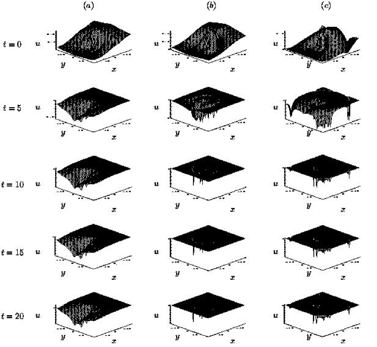
Figure 6: Propagating type structures corresponding to Eq. (89) at various instants: (a) $I_{1},I_{2}\neq 0$ (b) $I_{1}\neq 0,I_{2}=0$ (c) $I_{1}=0,I_{2}\neq 0$.

6.2(B) The choice $b=0$

In the general reduction, we have assumed $b\neq 0$. In this subsection, we derive certain interesting patterns by taking the symmetry parameter $b=0$. For this choice the symmetries are (vide Eq. (63))

$$\tau=a,\quad\xi=l,\quad\eta=n,\quad\phi=c(t,x,y)(1-u)^{2}.$$ (90)

The similarity transformations

$$z_{1}=nx-ly,\;\;z_{2}=ax-lt,\;\;u=1-\displaystyle{\frac{a}{w(z_{1},z_{2})+\int c(t,x,y)dt}},$$ (91)

are found by solving the characteristic equation associated with Eq. (90). Under the above set of transformations (91), Eq. (61) can be transformed to

$$lw_{z_{2}}+(l^{2}+n^{2})w_{z_{1}z_{1}}+a^{2}w_{z_{2}z_{2}}+2anw_{z_{1}z_{2}}+w-a=0.$$ (92)

The invariance of Eq. (92) under the one-parameter Lie group transformations leads to the infinitesimals

$$\tau=2a\displaystyle{\frac{n}{l}}c_{1}z_{2}-2\displaystyle{\frac{a^{2}}{l}}c_{1}z_{1}+c_{2},\quad\xi=-2a\displaystyle{\frac{n}{l}}c_{1}z_{1}+\displaystyle{\frac{2}{l}}(l^{2}+n^{2})c_{1}z_{2}-c_{3},$$

$$\phi=(c_{1}z_{1}+c_{4})\bar{w}+h(z_{1},z_{2}),$$ (93)

where $\bar{w}=w-a$ and the arbitrary function $h(z_{1},z_{2})$ satisfies the equation $lh_{z_{2}}+(l^{2}+n^{2})h_{z_{1}z_{1}}+a^{2}h_{z_{2}z_{2}}+2anh_{z_{1}z_{2}}$ $+h=0.$

Using the symmetries given in Eq. (93) one can construct a general similarity reduced ODE. However, as our aim is to show some interesting solutions we consider a lesser symmetry parameter group in the following.

Case (a): To begin with let us consider $c_{1}\neq 0$ and all other parameters $(c_{2},c_{3},c_{4})$ are zero in (93). Now solving the characteristic equation associated with the symmetries we obtain the following similarity variables

$$\zeta = \frac{a^{2}}{2}z_{1}^{2}+\frac{(l^{2}+n^{2})}{2}z_{2}^{2}-anz_{1}z_{2},$$

$$\bar{w} = e^{-\displaystyle{F(\zeta,z_{1})}}\Bigg{[}f(\zeta)-\displaystyle{\frac{(al)^{2}}{c_{1}}}\displaystyle{\int F(\zeta,z_{1})h(z_{1},z_{2})e^{\displaystyle{F(\zeta,z_{1})}}dz_{1}}\Bigg{]},$$ (94)

where $F(\zeta,z_{1})=-\displaystyle{\frac{1}{2a^{2}l}\Big{[}2(l^{2}+n^{2})\zeta-a^{2}l^{2}z_{1}^{2}\Big{]}^{\frac{1}{2}}}$. Using the above similarity transformations we deduce an ODE

$$\zeta f^{\prime\prime}+f^{\prime}+Bf=0,\quad B=\displaystyle{\frac{1}{2a^{2}l}}\Bigg{(}1-\displaystyle{\frac{l^{2}+n^{2}}{4a^{2}}}\Bigg{)},$$ (95)

where the prime stands for differentiation with respect to $\zeta$. Eq. (95) admits a time-dependent cylindrical wave solution of the form

$$f(\zeta)=I_{1}J_{0}(2\sqrt{B\zeta})+I_{2}Y_{0}(2\sqrt{B\zeta}).$$ (96)

From (96) we can provide the time-dependent solution to the original PDE through the transformations (94) and (91). The solution is plotted in Figs. (7) for various instants, exhibiting propagating spike like patterns.

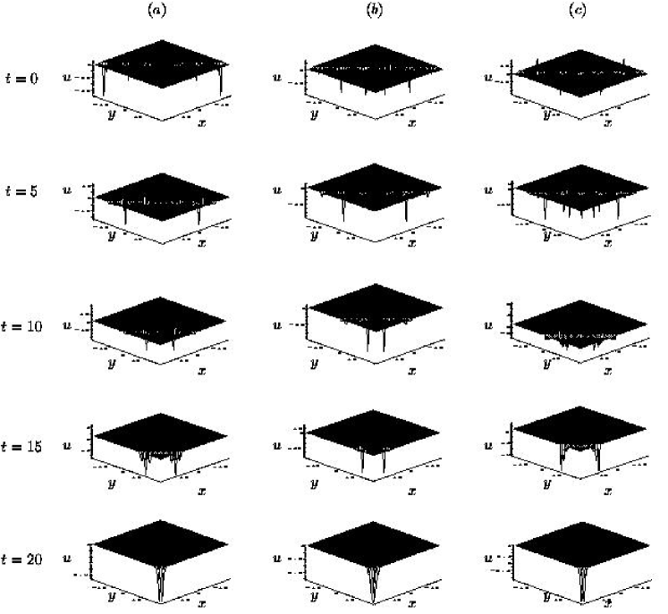
Figure 7: Bessel type propagating solutions for various instants as given by Eq. (96): (a) $I_{1},I_{2}\neq 0$, (b) $I_{1}\neq 0,I_{2}=0$ (c) $I_{1}=0,I_{2}\neq 0$.

Case (b): $c_{1}=0$.

The choice $c_{1}=0$ and $c_{2},c_{3},c_{4}\neq 0$ in Eq. (93) leads to the similarity transformations

$$\zeta=c_{3}z_{2}+c_{2}z_{1},\quad\bar{w}=e^{\displaystyle{kz_{2}}}\left[f(\zeta)+\frac{1}{c_{2}}\int h(z_{1},z_{2})e^{\displaystyle{k}z_{2}}dz_{2}\right],\;k=\frac{c_{4}}{c_{2}}$$ (97)

which transforms Eq. (92) into an ODE of the form

$$Af^{\prime\prime}+Bf^{\prime}+Cf=0,\quad A=(ac_{3})^{2}+(l^{2}+n^{2})c_{2}^{2}+2anc_{2}c_{3},$$

$$B=lc_{3}+2a^{2}kc_{3}+2anc_{4},\quad C=1+lk+(ak)^{2},\;\;^{\prime}=\frac{\displaystyle{d}}{\displaystyle{d\zeta}},$$ (98)

whose general solution is given by

$$f(\zeta)=I_{1}e^{\displaystyle{m_{1}\zeta}}+I_{2}e^{\displaystyle{m_{2}\zeta}},\quad m_{1,2}=-\frac{1}{2A}\left(B\pm\sqrt{B^{2}-4AC}\right),$$ (99)

and $\zeta$ is quadratic in time $t$. Substituting the similarity transformations (97) and (91) in (99) the solution to the original PDE (61) can be obtained.

Case (c): Propagating structures.

By assuming $n=c_{3}=0$ in Eq. (98), the ODE becomes

$$f^{\prime\prime}-k_{1}f=0,\quad k_{1}=-\displaystyle{\frac{1+lk+(ak)^{2}}{(lc_{2})^{2}}}.$$ (100)

Then, the system (61) is found to exhibit propagating structures and the corresponding solutions are given by

$$u=\left\{\begin{array}[]{lll}1-a\Bigg{\{}a+\exp\Big{[}\displaystyle{{k\left(ax-lt\right)}}\Big{]}\Bigg{[}I_{1}\cos(\sqrt{k_{1}}c_{2}ly)+I_{2}\sin(\sqrt{k_{1}}c_{2}ly)\Bigg{.}\Bigg{.}\\ \Bigg{.}\Bigg{.}\mskip 150.0mu+\displaystyle{\int\frac{h(z_{1},z_{2})}{c_{5}}}e^{\displaystyle{kz_{2}}}dz_{2}\Bigg{]}+\displaystyle{\int c(t,x,y)dt}\Bigg{\}}^{-1},\quad\quad k_{1}<0;\\[5.69054pt] 1-a\Bigg{\{}a+\exp\Big{[}\displaystyle{k\left(ax-lt\right)}\Big{]}\Bigg{[}I_{1}e^{\displaystyle{\sqrt{k_{1}}c_{2}ly}}+I_{2}e^{\displaystyle{-\sqrt{k_{1}}c_{2}ly}}\Bigg{.}\Bigg{.}\\ \Bigg{.}\Bigg{.}\mskip 150.0mu+\displaystyle{\int\frac{h(z_{1},z_{2})}{c_{5}}}e^{\displaystyle{kz_{2}}}dz_{2}\Bigg{]}+\displaystyle{\int c(t,x,y)dt}\Bigg{\}}^{-1},\quad\quad k_{1}>0;\\[5.69054pt] 1-a\Bigg{\{}a+\exp\Big{[}\displaystyle{k\left(ax-lt\right)}\Big{]}\Bigg{[}I_{1}c_{2}ly+I_{2}\Bigg{.}\Bigg{.}\\ \Bigg{.}\Bigg{.}\mskip 150.0mu+\displaystyle{\int\frac{h(z_{1},z_{2})}{c_{5}}}e^{\displaystyle{kz_{2}}}dz_{2}\Bigg{]}+\displaystyle{\int c(t,x,y)dt}\Bigg{\}}^{-1},\quad\quad k_{1}=0.\\[5.69054pt] \end{array}\right.$$ (107)

The presence of an additional function $h(z_{1},z_{2})$ in the solution (107) leads to a more general form. In particular, Eq. (107) exhibits the five classes of bounded travelling wave solutions reported by Brazhnik and Tyson [1999a] with specific choice of the parameters involved along with $h(z_{1},z_{2})=0$ and $c(t,x,y)=0$. The corresponding solutions are given below.

The simplest travelling wave solution (Fig. 8a)

$$u=1-\displaystyle{\frac{1}{1+A\exp\left[k\left(\displaystyle{ax-lt}\right)\pm\sqrt{k_{1}}c_{2}ly\right]}},\quad\quad k_{1}>0,\quad A=\displaystyle{\frac{I_{2}}{a}}\;\mbox{or}\;\displaystyle{\frac{I_{1}}{a}}$$ (108)

is constructed by assuming either $I_{1}=0$ or $I_{2}=0$. When $I_{1}=I_{2}(\neq 0)$, one obtains a V-wave pattern (Fig. 8b)

$$u=1-\displaystyle{\frac{1}{1+A\exp\left[\displaystyle{k\left(ax-lt\right)}\right]\cosh(\sqrt{k_{1}}c_{2}ly)}},\;\;k_{1}>0,\quad A=\displaystyle{\frac{2}{a}}.$$ (109)

A wavefront oscillating in space (Fig. 8c)

$$u=1-\displaystyle{\frac{1}{1+A\exp\left[\displaystyle{k\left(ax-lt\right)}\right]|\cos(\sqrt{k_{1}}c_{2}ly)|}},\quad A=\displaystyle{\frac{I_{1}}{a}}$$ (110)

exists for the choice $I_{2}=0$ and $k_{1}<0$. Further for $I_{1}\neq 0$ and $I_{2}=0$ we get a separatrix solution (Fig. 8d)

$$u=1-\displaystyle{\frac{1}{1+A|y|\exp\left[\displaystyle{k\left(ax-lt\right)}\right]}},\quad k_{1}=0,\quad A=\displaystyle{\frac{I_{1}lc_{2}}{a}}.$$ (111)

Finally, for positive $k_{1}$ with $I_{1}=-I_{2}$ the Y-wave solution (Fig. 8e)

$$u=1-\displaystyle{\frac{1}{1+A\exp\left[\displaystyle{k\left(ax-lt\right)}\right]|\sinh(\sqrt{k_{1}}c_{2}ly)|}},\quad A=\displaystyle{\frac{I_{1}}{a}}$$ (112)

exists. In each of the above solutions $A$ is a positive constant. As Fisher equation forms a basis for many nonlinear models, the above solutions are nothing but reminiscent of patterns from different fields. To mention a few, V-waves are characterized in the framework of geometrical crystal growth related models [Schwendeman, 1996] and in excitable media [Brazhnik & Davydov, 1995], while space oscillating fronts are relevant to cellular flame structures and patterns in chemical reaction diffusion systems [Scott & Showalter, 1992; Showalter, 1995]. Besides, excitable media supporting space-oscillating fronts are discussed by Brazhnik et al. [1996] with a geometrical model.

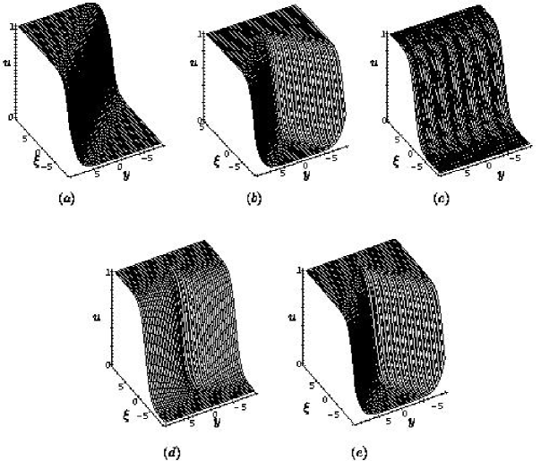
Figure 8: Five interesting classes of propagating wave patterns as obtained in ref.[Brazhnik & Tyson, 1999a], which follow from Eqs. (107): (a) Travelling waves, (b) V-waves, (c) Oscillating front, (d) Separatrix solution, (e) Y-waves with $\xi=k(ax-lt)$.

6.3 Relation between symmetries of $m=2$ case and of linear heat equation in 2-spatial dimensions

Proceeding in a similar fashion as that for the (1+1) dimensional Fisher equation as given in subsection 4.3 one obtains a mapping

$$z_{1}=t,\;z_{2}=x,\;z_{3}=y,\;w=\frac{1}{1-u}$$ (113)

by solving Eqs. (52) for the two spatial dimensional case. Eq. (113) then transforms the Fisher equation in 2-spatial dimensions to a 2-dimensional linear heat equation

$$v_{z_{1}}-v_{z_{2}z_{2}}-v_{z_{3}z_{3}}-v=0,\;w=1+v.$$ (114)

However, as in the case of the (1+1) dimensional GF equation, we have given an interpretation for the transformation (113) in terms of the Bäcklund transformation via Eq. (21).

7 The Nonintegrable (2+1) Dimensional GF Equation

One can make use of the same techniques that used for the integrable case to obtain some special solutions for the nonintegrable case ($m\neq 2$). To start with, we shall consider the general reductions. Due to the nonintegrable nature of the equation under consideration, the general reductions lead to ODEs of non-Painlevé type. However, we obtain certain special solutions, like plane wave solutions, static structures and localized structures under appropriate parametric restrictions.

7.1 General reductions

To begin with we derive a general similarity reduced ODE by assuming none of the parameters in (64) to be zero. The similarity variables thus obtained are

$$\displaystyle{z_{1}=\frac{b}{2}(x^{2}+y^{2})+ly-nx,\quad z_{2}=-t-\frac{a}{b}\sin^{-1}\left(\frac{n-bx}{\sqrt{l^{2}+n^{2}+2bz_{1}}}\right),}$$

$$u=w(z_{1},z_{2}).$$ (115)

Under the transformations (115) the reduced PDE in two independent variables takes the form

$$\displaystyle{w_{z_{2}}+2bw_{z_{1}}+(2bz_{1}+l^{2}+n^{2})w_{z_{1}z_{1}}+\frac{a^{2}w_{z_{2}z_{2}}}{2bz_{1}+l^{2}+n^{2}}}+\displaystyle{\frac{m}{1-w}}$$

$$\times\displaystyle{\left[(2bz_{1}+l^{2}+n^{2})w_{z_{1}}^{2}+\frac{a^{2}w_{z_{2}}^{2}}{2bz_{1}+l^{2}+n^{2}}\right]-w+w^{2}} =0.$$ (116)

Again looking the invariance properties of Eq. (116) we get the following infinitesimals:

$$\tau=c_{1},\quad\xi=0,\quad\phi=0.$$ (117)

These infinitesimals reduce Eq. (116) to an ODE

$$4b^{2}\left(\zeta f^{\prime\prime}+f^{\prime}+\frac{m\zeta}{1-f}f^{{}^{\prime}2}\right)+f-f^{2}=0$$ (118)

under a set of similarity transformations

$$\zeta=\bar{z}_{1},\quad w=f(\zeta),\quad\bar{z}_{1}=2bz_{1}+l^{2}+n^{2}.$$ (119)

As Eq. (118) is not integrable, we look for special reductions with lesser number of parameters involved.

7.2 Special reductions

For the special case $b=0$ the infinitesimals obtained are $\tau=a,\xi=l,\;\eta=n,\;\phi=0$. The associated similarity transformations $z_{1}=nx-ly,\;z_{2}=ax-lt,\;u=w(z_{1},z_{2})$ reduces the Fisher type equation (61) to a PDE

$$lw_{z_{2}}+(l^{2}+n^{2})w_{z_{1}z_{1}}+a^{2}w_{z_{2}z_{2}}+2anw_{z_{1}z_{2}}+\frac{m}{1-w}$$

$$\times\displaystyle{\left[(l^{2}+n^{2})w_{z_{1}}^{2}+a^{2}w_{z_{2}}^{2}+2anw_{z_{1}}w_{z_{2}}\right]+w-w^{2}} =0$$ (120)

in two independent variables $z_{1}$ and $z_{2}$. Applying classical Lie algorithm on Eq. (120) one obtains the following infinitesimals

$$\tau=c_{2},\quad\xi=\frac{n(c_{1}+c_{2})}{a},\quad\phi=0.$$ (121)

The corresponding similarity variables, $\zeta=-ac_{2}z_{1}+n(c_{1}+c_{2})z_{2}$ and $w=f(\zeta)$, reduce Eq. (120) to

$$A\bar{f}^{\prime\prime}+B\bar{f}^{\prime}-\frac{Am}{\bar{f}}\bar{f}^{{}^{\prime}2}-\bar{f}+\bar{f}^{2}=0,$$ (122)

with $\bar{f}=1-f,\;A=a^{2}(c_{1}^{2}n^{2}+c_{2}^{2}l^{2}),\;B=nl(c_{1}+c_{2})$ and prime stands for differentiation with respect to $\zeta.$ Because of the nonintegrable nature of Eq. (122), we look for subcases by assuming one or more of the vector fields to be zero. In the following we report some of the nontrivial cases.

7.2(A) Plane wave solutions

For $m=0$, making use of a similar procedure as in the previous case we can obtain the plane wave solution. That is, $m=0$ leads to the ODE for $\bar{\zeta}=\zeta/\sqrt{A}$

$${\bar{f}}^{\prime\prime}+\frac{B}{\sqrt{A}}{\bar{f}}^{\prime}-\bar{f}+\bar{f}^{2}=0.$$ (123)

It is then straightforward to check that for $B/\sqrt{A}=5/\sqrt{6}$, Eq. (123) satisfies the Painlevé property so that the solution to the original PDE is found to be

$$u(x,y,t)=1-\Bigg{[}1+\frac{k}{\sqrt{6}}\exp\Bigg{(}\frac{n(c_{1}+c_{2})(ax-lt)-ac_{2}(ly-nx)}{\sqrt{6A}}\Bigg{)}\Bigg{]}^{-2}.$$ (124)

Here we obtain a propagating plane wave and the pattern is plotted in (Figs. 9).

Figure 9: An exact propagating plane wave solution Eq. (124) at different instants of time: (a) $t=0$, (b) $t=5$, (c) $t=10$, (d) $t=15$.

7.2(B) Static and localized structures

Substituting $c_{1}=-c_{2}$ in (121), we obtain the similarity transformations $\zeta=z_{1},\;w=f(\zeta)$. This transforms Eq. (120) to an ODE

$$\bar{f}^{\prime\prime}-\displaystyle{\frac{m}{\bar{f}}}\bar{f}^{\prime}{{}^{2}}-A\bar{f}(1-\bar{f})=0,\;A=\frac{1}{l^{2}+n^{2}}.$$ (125)

For Eq. (125), in addition to the elliptic function solutions of the form tabulated in Table 1, we obtain a particular planar solitary wave solution (Fig. 10)

$$u=1-\frac{3-2m}{2-2m}\left[\mbox{sech}^{2}\left(I_{2}-\frac{(nx-ly)}{2}\sqrt{\frac{A}{1-m}}\right)\right],\;m<1.$$ (126)

We note the solutions given in (124) and (126) are 2-dimensional generalizations of (40) and (46) respectively.

Figure 10: Fig. 10. A planar solitary wave solution for Eq. (125) in the particular limit.

Besides the above, the choice $b=0,\;a=0,\;l=0$ reduces the (2+1) dimensional Fisher equation (61) to that in (1+1) dimensions for $m\neq 2$.

Table 2: Elliptic Function Solutions of Eq. (42) for $m=1/2$.

S.No.	Order of Roots	Function $v(z)$	modulus $k$
1.	$c_{1}>c_{2}>0\geq v$	$v=c_{1}-\displaystyle{\frac{c_{1}}{{sn}^{2}\left(\displaystyle{\frac{\sqrt{c_{1}}}{2}}(z-I_{2}),k\right)}}$	$\displaystyle{k^{2}=\frac{c_{1}-c_{2}}{c_{1}}}$
2.	$c_{1}>c_{2}>0>v$	$v=\displaystyle{\frac{c_{2}{sn}^{2}\left(\displaystyle{\frac{\sqrt{c_{1}}}{2}}(z-I_{2}),k\right)}{{sn}^{2}\left(\displaystyle{\frac{\sqrt{c_{1}}}{2}}(z-I_{2}),k\right)-1}}$	$\displaystyle{k^{2}=\frac{c_{1}-c_{2}}{c_{1}}}$
3.	$c_{1}\geq v>c_{2}>0$	$v=\displaystyle{\frac{c_{1}c_{2}}{c_{1}-(c_{1}-c_{2})sn^{2}\left[\displaystyle{\frac{\sqrt{c_{1}}}{2}}(z-I_{2}),k\right]}}$	$k^{2}=\displaystyle{\frac{c_{1}-c_{2}}{c_{1}}}$
4.	$c_{1}>v\geq c_{2}>0$	$v=c_{1}-(c_{1}-c_{2})sn^{2}\left[\displaystyle{\frac{\sqrt{c_{1}}}{2}}(z-I_{2}),k\right]$	$k^{2}=\displaystyle{\frac{c_{1}-c_{2}}{c_{1}}}$

8 Nonclassical Reductions

Generally, for many PDEs there exist symmetry reductions that are not obtained by using the classical Lie group method. As a consequence, there have been several generalizations of the classical Lie group method for symmetry reductions. Bluman and Cole [1969], then proposed the so-called non-classical method of group-invariant solutions in the study of symmetry reductions of a linear heat equation. An algorithm for calculating the determining equations associated with the nonclassical method was presented by Clarkson and Mansfield [1993]. This procedure has been applied to several nonlinear systems and in some cases, such as the Boussinesq equation, the Burgers’ equation and the FitzHugh-Nagumo equation, new similarity reductions not obtainable through classical symmetries have been found [Levi & Winternitz, 1989; Arrigo et al. 1993; Nucci & Clarkson, 1992] (see also Mansfield et al. [1998] and references therein). In the classical method we consider the infinitesimal generator, associated with the one-parameter Lie group of transformations,

$$V=\xi(t,x,u)\partial_{x}+\tau(t,x,u)\partial_{t}+\phi(t,x,u)\partial_{u}$$ (127)

which leaves the system (13) invariant. But in the nonclassical method, one requires the given equation (13) and the surface condition

$$\xi(t,x,u)u_{x}+\tau(t,x,u)u_{t}-\phi(t,x,u)=0$$ (128)

together to be invariant under the transformation with the infinitesimal generator (127). In this case one may obtain a larger set of solutions than that for the classical method. Moreover, significant progress has been made in the study of nonclassical symmetries for nonlinear PDEs of diffusive type. To mention a few, Gandarias and Bruzón, [1999] have obtained several solutions for a family of Cahn-Hilliard equations that are not invariant under any Lie group admitted by the equation. In a similar fashion, separable new solutions that are not obtainable via classical method have been reported for a mathematical model [Gandarias, 2001] of fast diffusion through nonclassical method. This prompts us to look for nonclassical symmetries associated with the GF equation (9).

8.1 The (1+1) dimensional Fisher equation

There are two types of nonclassical symmetries: those where the infinitesimal $\tau$ is non-zero and those where it is zero. In the first case, we can assume without loss of generality that $\tau=1$, while in the second case we can assume $\xi\neq 0$ and $\tau=0$. In the following we investigate them separately.

8.1(A) The case ${\bf\tau\neq 0}$

We set $\tau=1$ in the invariant surface condition without loss of generality and use it together with its differential consequences to eliminate $u_{t}$ and so Eq. (13) takes the form

$$u_{xx}=\phi-\xi u_{x}-\frac{m}{1-u}u_{x}^{2}-u+u^{2}.$$ (129)

Applying the classical Lie algorithm to (129) and eliminating the highest derivative involving the variable $x$, the coefficients of the linearly independent expressions in the remaining derivatives are set equal to zero. From the resultant set of determining equations for $\xi,\tau,$ and $\phi$, which are in general nonlinear, we get

$$\tau=1,\quad\xi=b,\quad\phi=d(t,x)(1-u)^{2},\quad m=2,$$ (130a)

$$\tau=1,\quad\xi=b,\quad\phi=0,\quad m\neq 2,$$ (130b)

where $b$ is an arbitrary constant. In Eq. (130a), $d(t,x)$ satisfies $d_{t}-d_{xx}-d=0$.

The corresponding similarity variables for the $m=2$ case are

$$z=x-bt,\quad u=1-\displaystyle{\frac{1}{w(z)+\int d(t,x)dt},}$$ (131)

which are similar to the ones obtained by the classical method earlier in Sec.4. Thus we are lead to the similarity reduced differential equation

$$\displaystyle{\bar{w}^{\prime\prime}+b\bar{w}^{\prime}+\bar{w}=0},\;\bar{w}=w-1,\;^{\prime}=d/dz,$$ (132)

which is similar to (31) and the results then follows as before. Similar is the case with $m\neq 2$. Thus both classical and nonclassical reductions lead to the same solutions for the present system.

8.1(B) The case ${\bf\tau=0},\;{\bf\xi\neq 0}$

Let $\tau=0$ and $\xi\neq 0$. We then set $\xi=1$, without loss of generality. The invariance surface condition simplifies the Fisher equation to

$$u_{t}-\phi_{x}-\phi\phi_{u}-\frac{m}{1-u}\phi^{2}-u+u^{2}=0.$$ (133)

Applying the classical Lie algorithm to the above equation we end up with a more complicated nonlinear PDE

$$\phi_{t}-\phi_{xx}-2\phi\phi_{xu}-\phi^{2}\phi_{uu}+u(1-u)\phi_{u}+(2u-1)\phi$$

$$-\frac{2m}{1-u}\phi\phi_{x}-\frac{m}{1-u}\phi^{2}\phi_{u}-\frac{m}{(1-u)^{2}}\phi^{3} =0.$$ (134)

This system is considerably more complex than the system (13) and hence cannot be solved in general. We have made different ansätze for $\phi(t,x,u)$ and found that all of them lead to only the group invariant solutions found by the classical algorithm.

However, for the $m=0$ case, by assuming $\phi$ to be independent of $x$ and $t$ we get $\phi=u\sqrt{\displaystyle{\frac{2u}{3}-1}},\;\tau=0,\;\xi=1$ which is different from that obtained through the classical method. However this choice leads to a singular solution of the form

$$u=\frac{3}{2}\sec^{2}\left(\frac{x+c}{2}\right).$$ (135)

8.2 The (2+1) dimensional GF equation

We extend the nonclassical symmetry analysis to the (2+1) dimensional Fisher equation (61) and in this analysis there are three cases to consider, namely, (i) $\tau\neq 0$, (ii) $\tau=0,\;\;\eta\neq 0$, and (iii) $\tau=0,\;\;\eta=0,\;\;\xi\neq 0$.

8.2(A) The case ${\bf\tau\neq 0}$

We use the invariance surface condition

$$u_{t}=\phi-\xi u_{x}-\eta u_{y}$$ (136)

with its differential consequences to eliminate $u_{t}$. Applying the classical Lie algorithm to the Fisher equation

$$\phi-\xi u_{x}-\eta u_{y}-u_{xx}-u_{yy}-\frac{m}{1-u}(u_{x}^{2}+u_{y}^{2})-u+u^{2}=0$$ (137)

and then equating coefficients of various powers of derivatives of the dependent variable $u$ we have a set of determining equations. Solving them we get finally

$$\tau=1,\quad\xi=a_{3}y+a_{4},\quad\eta=-a_{3}x+c_{4},\quad\phi=d(t,x,y)(1-u)^{2},\quad m=2,$$ (138a)

$$\tau=1,\quad\xi=a_{3}y+a_{4},\quad\eta=-a_{3}x+c_{4},\quad\phi=0,\quad m\neq 2.$$ (138b)

Here $d(t,x,y)$ satisfies the equation $d_{t}-d_{xx}-d_{yy}-d=0$ and $a_{3},a_{4},c_{4}$ are arbitrary constants. Comparing this set of symmetries with that obtained by the classical method we find that they are similar to the latter case. So the similarity reductions will reduce the PDE to the same ODE as that obtained by the classical method.

8.2(B) The case ${\bf\tau=0}$, ${\bf\eta\neq 0}$

Here we set $\eta=1$, without loss of generality, and analogous to the above procedure we use the above choice to eliminate all $y$-derivatives. Then applying the classical Lie algorithm to the resulting equation we obtain a more complicated nonlinear PDE. Solving the resultant system of determining equations we obtain the following symmetries

$$(i)\quad \tau=0,\quad\xi=c_{1},\qquad\;\;\eta=1,\quad\phi=0,$$ (139a)

$$(ii)\quad \tau=0,\quad\xi=\pm\frac{1}{\sqrt{2}},\quad\eta=1,\quad\phi=0,\;$$ (139b)

for all values of $m$. The similarity reduction variables $z_{1}=c_{1}y-x,\;z_{2}=t,\;u=w(z_{1},z_{2})$ associated with (139a) reduces the GF equation in 2-spatial dimensions to that in 1-spatial dimension. Similarly, the similarity transformations $z_{1}=\pm\sqrt{2}y-x,\;z_{2}=t,\;u=w(z_{1},z_{2})$ for (139b) again reduces the original PDE to that in 1-dimension and hence the results follow as in the case of the classical method.

8.2(C) The case ${\bf\tau=0}$, ${\bf\eta=0}$, ${\bf\xi\neq 0}$

In this case we set $\xi=1$, without loss of generality, and as above we make use of the invariance condition $u_{x}=\phi$ to eliminate all $x$-derivatives. Then we apply the classical Lie algorithm to the resulting equation and we get a nonlinear PDE of the form

$$-\phi_{t}+\phi_{xx}+\phi_{yy}+\phi_{uu}(\phi^{2}+u_{y}^{2})+(1-2u+2\phi_{ux})\phi+2\phi_{uy}u_{y}-u(1-u)\phi_{u}$$

$$+\frac{m}{(1-u)}\Big{[}\frac{\phi}{(1-u)}(u_{y}^{2}+\phi^{2})+\phi_{u}(u_{y}^{2}+\phi^{2})+2\phi_{y}u_{y}+2\phi\phi_{x}\Big{]} =0.$$ (140)

Solving the system of determining equations we obtain $\phi=0$ $\forall\;m$. Thus the (2+1)-dimensional GF type equation, under the similarity transformation $z_{1}=y,\;z_{2}=t,\;u=w(z_{1},z_{2})$ reduces to that in (1+1)-dimensions and hence the results as in the case of the classical Lie algorithm case follow.

9 Generalized Conditional Symmetry Reductions

Recently Fokas and Liu [1994a,b] proposed the notion of Generalized Conditional Symmetry (GCS) and applied it to construct some physically interesting exact solutions of certain nonlinear nonintegrable PDEs. Such exact solutions are of primary importance because they identify certain interesting and novel physical phenomena and moreover such solutions may be hard to identify or may not be quite transparent from the numerical solution of a nonlinear PDE. In this method the PDE is reduced to an ODE in terms of certain types of generalized conditional symmetries. Indeed the GCS can be considered as a natural generalization of the nonclassical method just as the generalized symmetry method [Olver, 1986] is considered as a generalization of the Lie-point symmetry method. Particularly, for the reaction diffusion type equations, several new separable solutions that cannot be obtained via the non-classical and non-local symmetry methods have been derived through this method [Qu, 1997; Qu, 1999a,b; Chou & Ku, 1999; Qu et al., 2000]. Further, it is recently shown that the GCS method is the most efficient tool for solving the problem of dimensional reduction of initial value problems for evolutionary type PDEs in a purely algebraic way [Zhadanov & Andreitsev, 2000]. Motivated by these facts we investigate the existence of generalized conditional symmetries, if any, for the GF equation.

9.1 The method

Let $K(t,u)$ denotes a function that depends on a differentiable manner of $t,u,u_{x},u_{xx},\ldots$. The function $\sigma(t,x,u)$ is a generalized symmetry of the evolution equation $u_{t}=K(t,u)$ iff

$$\frac{\partial\sigma}{\partial t}+[K,\sigma]=0,$$ (141)

when $u_{t}=K(t,u)$, where $[K,\sigma]=\sigma^{\prime}K-K^{\prime}\sigma,$ and the prime denotes the Gateaux derivative. The function $\sigma(t,x,u)$ is a GCS of equation (13) if there exists a function $A$ such that

$$\frac{\partial\sigma}{\partial t}+[K,\sigma]=A(t,x,u,\sigma),\quad A(t,x,u,0)=0,$$ (142)

where $K(t,u)$, and $\sigma(t,x,u)$ are differentiable functions of $t,x,u,u_{x},u_{xx},\ldots$ and $A(t,x,u,\sigma)$ is a differentiable function of $t,x,u,u_{x},u_{xx}$,…, and $\sigma,\sigma_{x},\sigma_{xx},\ldots$ It is obvious from (142) that Eq. (141) admits a GCS $\sigma$ iff

$$\sigma^{\prime}K\mid_{\sigma=0}=0,$$ (143)

provided $\sigma$ is explicitly independent of time $t$.

9.2 The (1+1)- dimensional GF equation

Let the Fisher equation admits a GCS of the form

$$\sigma=u_{xx}+H(u)u_{x}^{2}+F(u)u_{x}+G(u),$$ (144)

where $H(u),F(u)$ and $G(u)$ are arbitrary functions $u$. Substituting (144) into (143) one gets

$$\left[H_{uu}-2H(2H_{u}-H^{2})-\frac{m}{(1-u)^{2}}\left(\frac{2}{1-u}-3H\right)+\frac{m}{1-u}\left(H_{u}-2H^{2}\right)\right]u_{x}^{4}$$

$$+\Bigg{[}F_{uu}-2HF_{u}-4F(H_{u}-H^{2})+\frac{m}{1-u}(F_{u}+4FH)+\frac{4mF}{(1-u)^{2}}\Bigg{]}u_{x}^{3}$$

$$-\Bigg{[}G_{uu}-2F(F_{u}-HF)-4G(H_{u}-H^{2})+(2u-1)H-u(1-u)H_{u}\Bigg{.}$$

$$\Bigg{.}+\frac{m}{1-u}\left(4HG-2F^{2}+G_{u}\right)+\frac{5mG}{(1-u)^{2}}\Bigg{]}u_{x}^{2}-\Bigg{[}\left(u(1-u)+2G\right)F_{u}\Bigg{.}$$

$$\Bigg{.}+4FG\left(\frac{m}{1-u}-H\right)\Bigg{]}u_{x}-u(1-u)G_{u}+(1-2u)G$$

$$+2G^{2}(H-\frac{m}{1-u}) =0.$$ (145)

Equating coefficients of various powers of $u_{x}$ to zero and then solving the resulting overdetermined equations we get

$$H(u)=\displaystyle{\frac{m}{1-u}},\quad G(u)=u(1-u),\quad F(u)=c_{1},\quad\forall\;m,$$ (146)

where $c_{1}$ and $c_{2}$ are arbitrary constants. The corresponding GCS are

$$\sigma=u_{xx}+\frac{m}{1-u}u_{x}^{2}+c_{1}u_{x}+u-u^{2}.$$ (147)

With the above some exact solutions can be constructed. The ODE $\sigma=0$ is solved to obtain $u$ as a function of $x$ with integration constants dependent on time $t$ alone. Then substituting this solution into the governing equation, the time evolution of these time-independent constants are determined. The exact solutions are then obtained by solving these systems.

The GCS (147) leads to

$$u^{\prime\prime}+\frac{m}{1-u}u^{\prime 2}+c_{1}u^{\prime}+u-u^{2}=0$$ (148)

which cannot be integrated as such except for $m=2$. Thus for $m=2$, we obtain

$$u=1-\left[1+A(t)e^{m_{1}x}+B(t)e^{m_{2}x}\right]^{-1},\quad m_{1,2}=\frac{-c_{1}\pm\sqrt{c_{1}^{2}-4}}{2}.$$ (149)

Substituting (149) into the Fisher equation (13) we get

$$\displaystyle{u=1-\left(1+Ae^{\displaystyle[(m_{1}^{2}+1)t+m_{1}x]}+Be^{\displaystyle[(m_{2}^{2}+1)t+m_{2}x]}\right)^{-1}},$$ (150a)

$$\displaystyle{m_{1,2}=\frac{c_{1}\pm\sqrt{c_{1}^{2}-4c_{2}}}{2}},$$ (150b)

for $m=2$. We wish to mention that the solution (150a) can be recovered from the linear heat equation Wang et al. [1996] and the results are similar to that obtained through the classical algorithm. Further Eq. (150b) is similar to Eq. (37) and hence we obtain the various propagating structures already discussed through the classical method.

Eq. (148) is of non-Painlevé type for all other values of m ($\neq 2$) and is similar to (39) and hence the previous results follow. Thus GCS reductions lead to the same results as that obtained through the classical method for the modified perturbed GF equation.

10 Conclusions

In this paper, we have investigated the integrability/symmetry properties of the generalized Fisher type nonlinear reaction-diffusion equation in both (1+1) and (2+1) dimensions. The singularity structure analysis singles out the $m=2$ case as the only system parameter for which the GF equation is free from movable critical singular manifolds. Further a Bäcklund transformation for the integrable case is shown to linearize the GF equation to the linear heat equation. The symmetry analysis shows that the system under consideration possesses interesting Lie point symmetries that lead to the infinite-dimensional Lie algebra for the integrable case, thereby exhibiting various interesting patterns and dynamics, and giving rise to a group theoretical interpretation for the system. In addition to the above, we have given exact and numerical solutions for specific choices of the nonintegrable case. Our studies on the GF equation reveals the existence of a large number of interesting wave patterns, static and localized structures. We have also carried out the nonclassical and generalized conditional symmetry reductions.

References

Ablowitz, M.J. & Zeppetella, A. [1979] ”Explicit solution of Fisher’s equation for a special wave speed”, Bull. Math. Biol., 41, 835-840.

Ablowitz, M. J. & Clarkson, P. A. [1991] ”Solitons: Nonlinear Evolution Equations and Inverse Scattering” (Cambridge University Press, Cambridge).

Arrigo, D.J., Broadbridge, P. & Hill, J.M. [1993] ”Nonclassical symmetry solutions and the methods of Bluman-Cole and Clarkson and Kruskal”, J. Math. Phys., 34, 4692-4703.

Bindu, P.S., Senthilvelan, M. & Lakshmanan, M. [2001] ”Singularity structures, symmetries and integrability aspects of generalized Fisher type nonlinear diffusion equation”, J. Phys. A: Math.
 Gen., 34, L689-L696.

Bindu, P.S. & Lakshmanan, M. [2002] ”Symmetries and integrability properties of generalized Fisher type nonlinear diffusion equation, Proceedings of the Institute of Mathematics of NAS, Ukraine, Eds. Nikitin, A.G., Boyko, V.M. & Popovych, R.O., Part -1, 43, 36-48.

Bluman, G.W. & Cole, J.D. [1969] ”The general similarity solutions of the heat equation”, J. Math. Mech., 18, 1025-1042.

Bluman, G.W. & Kumei, S. [1989] ”Symmetries and Differential Equations” (Springer-Verlag, New York).

Brazhnik, P.K. & Davydov, V.A. [1995] ”Non-spiral autowave structures in unrestricted excitable media”, Phys. Lett. A., 199, 40-44.

Brazhnik, P.K., Fan, S. & Tyson, J.J. [1996] ”Nonspiral excitation waves beyond the eikonal approximation”, Phys. Rev. E., 54, 4338-4346.

Brazhnik, P.K. & Tyson, J.J. [1999a] ”Travelling waves and static structures in a two-dimensionsal exactly solvable reaction-diffusion system”, J. Phys. A: Math. Gen., 32, 8033-8044.

Brazhnik,P.K. & Tyson, J.J. [1999b] ”On travelling wave solutions of Fisher’s equation in two spatial dimensions”, SIAM. J. Appl. Math., 60, 371-391.

Calogero, F. [1991] ”Why are Certain Nonlinear PDEs Both Widely Applicable and Integrable?”, in What is Integrability? Ed. V. E.  Zakharov, (Springer-Verlag, Berlin), p1-62.

Chou, K.S. & Qu, C.Z. [1999] ”Symmetry groups and separation of variables of a class of nonlinear diffusion-convection equations”, J. Phys. A: Math. Gen., 32, 6271-6286.

Clarkson, P.A. & Mansfield, E.L. [1993] ”Symmetry reductions and exact solutions of a class of nonlinear heat equations”, Physica D, 70, 250-288.

Fokas, A.S. & Yortsos, Y.C. [1982] ”On the exactly solvable equation $S_{t}=[(\beta S+\gamma)^{-2}S_{x}]_{x}+\alpha(\beta S+\gamma)^{-2}S_{x}$ occuring in two-phase flow in porous media”, SIAM J. Appl. Math., 42, 318-332.

Fokas, A.S. & Liu, Q.M. [1994a] ”Nonlinear interaction of travelling waves of nonintegrable equations”, Phys. Rev. Lett., 72, 3293-3296.

Fokas, A.S. & Liu, Q.M. [1994b] ”Generalized conditional symmetries and exact solutions of nonintegrable equations”, Theor. Math. Phys., 99, 263-277.

Gandarias, M.L. & Bruzón, M.S. [1999] ”Nonclassical symmetries for a family of Cahn-Hilliard equations”, Phys. Lett. A, 263, 331-337.

Gandarias, M.L. [2001] ”New symmetries for a model of fast diffusion”, Phys. Lett. A, 286, 153-160.

Grimson, M.J. & Barker, G.C. [1994] ”Continuum model for the spatiotemporal growth of bacterial colonies”, Phys. Rev. E., 49, 1680-1684.

Head, A. [1993] ”LIE: a PC program for Lie analysis of differential equations”, Comput. Phys. Commun., 77, 241-248.

Lakshmanan, M. & Rajasekar, S. [2003] ”Nonlinear Dynamics: Integrability, Chaos, and Patterns”, (Springer-Verlag, Berlin).

Levi, D. & Winternitz, P. [1989] ”Non-classical symmetry reduction: example of Boussinesq equation”, J. Phys. A: Math. Gen., 22, 2915-2924.

Mansfield, E.L., Reid, G.J. & Clarkson, P.A. [1998] ”Non-classical reductions of a (3+1) dimensional cubic nonlinear Schrödinger equation”, Compt. Phys. Comm., 115, 460-488.

Mathews, P.M. & Lakshmanan, M. [1974] ”On a unique nonlinear oscillator”, Qt. Appl. Math., 32, 215-218.

Murphy, G. M. [1969] ”Ordinary Differential Equations and Their Solutions” (Affiliated East-West Press, New Delhi).

Murray, J.D. [1989] ”Mathematical Biology” (Springer-Verlag, Berlin).

Nucci, M.C. & Clarkson, P.A. [1992] ”The nonclassical method is more general than the direct method for symmetry reductions: An example of the FitzHugh-Nagumo equation”, Phys. Lett. A, 164, 56-59.

Olver, P.J. [1986] ”Applications of Lie Groups to Differential Equations” (Springer-Verlag, New York).

Qu, C.Z. [1997] ”Group classification and generalized conditional symmetry reduction of the nonlinear diffusion-convection equation with a nonlinear source”, Stud. Appl. Math., 99, 107-136.

Qu, C.Z. [1999a] ”New generalized conditional symmetry reductions and exact solutions of the nonlinear diffusion-convection-reaction equations”, Commun. Theor. Phys., 31, 581-588.

Qu, C.Z. [1999b] ”Reductions and exact solutions of some nonlinear partial differential equations under four types of generalized conditional symmetries”, J. Austral. Math. Soc. B, 40, 1-42.

Qu, C.Z., Zhang, S. & Liu, R. [2000] ”Separation of variables and exact solutions to quasilinear diffusion equations with nonlinear source”, Physica D, 144, 97-123.

Rosen, G. [1982] ”Method for the exact solution of a nonlinear diffusion-convection equation”, Phys. Rev. Lett., 49, 1844-1847.

Sachdev, P.L. [1987] ”Nonlinear Diffusive Waves” (Cambridge University Press, Cambridge).

Schwendeman, D.W. [1996] ”A front dynamics approach to curvature-dependent flow”, SIAM. J.
 Appl. Math., 56, 1523-1538.

Scott, S.K. & Showalter, K. [1992] ”Simple and complex propagating reaction-diffusion front”, J. Chem. Phys., 96, 8702-8711.

Scott, A.C. [ 1999] ”Nonlinear Science: Emergence and Dynamics of Coherent Structures” (Oxford University Press, Oxford).

Showalter, K. [1995] ”Quadratic and cubic reaction-diffusion fronts”, Nonlinear. Sci. Today, 4, 1-10.

Walgraef, D. [1996] ”Spatiotemporal Pattern Formation” (Springer-Verlag, NewYork).

Wang, X.Y., Fan, S. & Kyu, T. [1996] ”Complete and exact solutions of a class of nonlinear diffusion equations and problem of velocity selection”, Phys. Rev. E., 56, R4931-R4934.

Weiss, J., Tabor, M. & Carnevale, G. [1983] ”The Painlevé property for partial differential equations”, J. Math. Phys., 24, 522-526.

Whitham, G.B. [1974] ”Linear and Nonlinear Waves” (Wiley, NewYork).

Zhadanov, R.Z. & Yu Andreitsev, A. [2000] ”Non-classical reductions of intial-value problems for a class of nonlinear evolution equations”, J. Phys. A: Math. Gen., 33, 5763-5781.