When Chaos Meets Computers
Abstract
This paper focuses on an interesting phenomena when chaos meets computers. It is found that digital computers are absolutely incapable of showing true long-time dynamics of some chaotic systems, including the tent map, the Bernoulli shift map and their analogues, even in a high-precision floating-point arithmetic. Although the results cannot directly generalized to most chaotic systems, the risk of using digital computers to numerically study continuous dynamical systems is shown clearly. As a result, we reach the old saying that “it is impossible to do everything with computers only”.
1 Introduction
This paper focuses on an interesting phenomena when chaos meets computers. When some chaotic systems are realized in digital computers, their true long-time dynamics cannot be exhibited at all, even in a high-precision floating-point arithmetic. Although the results cannot directly generalized to most other chaotic systems, the risk of using digital computers to numerically study continuous dynamical systems is exposed. Actually, in [1, Chap. 3], we have shown some more subtle dynamical degradation of generic piecewise linear chaotic maps realized with fixed-point finite precision in digital computers. Although the phenomena discussed in this paper is completely different from those studied in [1, Chap. 3], the essential reason of both cases can be attributed to the use of the multiplication factor 2 and its powers. Why is 2 a magic number? It is because all digital computers are based on binary arithmetic, in which a multiplication with is equal to the left bit-shifting operation , which may eat precision bits in each digital chaotic iteration if there does not exist a bit-compensation operation in the chaotic equation.
Two well-known piecewise linear chaotic maps, the Tent map and the Bernoulli shift map, are studied in this paper. It is rigorously proved that all chaotic orbits of the two maps will converge to zero within a limited number of iterations, and that the average and maximal numbers of iterations to reach such a convergence are uniquely determined by details of the involved digital arithmetic. In addition, it is found that the average number is generally much smaller than the maximal one, when the initial condition distributes uniformly in the space of all valid floating-point numbers. The results on the Tent map and the Bernoulli shift map can be directly extended to other analogue chaotic maps, including the V-map , the reflected Bernoulli map , and the Baker map (considering Bernoulli shift map is the -transformation of the Baker map) [2]. Note that the case of the Bernoulli shift map (also called doubling map) has been well-known to chaos community [3], but the case of the Tent map not yet. In fact, even for the Bernoulli shift map, there does not exist a quantitatively analysis on the long-time dynamics of the map evolving in digital computers. We hope this paper can help to clarify some questions.
2 Real Numbers in Digital Computers
As we know, digital computers adopt binary format to represent numbers. For real numbers, there are two kinds of representation formats: fixed-point format, and floating-point format. The fixed-point format is more suitable for integers or real numbers with a fixed precision, and the floating-point format is suitable for real numbers with a higher and variable precision. Accordingly, there are two kinds of digital arithmetic techniques. Because most simulation softwares of chaotic systems use floating-point arithmetic, we will not discuss fixed-point arithmetic in this paper. Actually, for the problem studied in this paper, the condition under floating-point arithmetic is much more complicated than that under fixed-point arithmetic, and the major results can be easily extended to fixed-point arithmetic.
In today’s digital world, the floating-point arithmetic has been standardized by IEEE and ANSI in 1985 [4], and almost all software and hardware implementations of floating-point arithmetic obey this standard to represent the real numbers. In the IEEE/ANSI floating-point standard, two different floating-point formats are defined: single-precision and double-precision. The single-precision format uses 32 bits to represent a real number, and the double-precision format uses 64 bits. To realize a higher simulation precision, generally double-precision is used for the study of chaotic systems. Thus, this paper will focus on double-precision floating-point arithmetic, and briefly call it floating-point arithmetic. Note that the extension from double-precision floating-point arithmetic to single-precision arithmetic is very easy.
Following the IEEE/ANSI floating-point standard, almost all real numbers are stored in the following normalized format:
| (1) |
where means a binary number and is called the fraction of the mantissa. There are five types of special values that are not represented in the above normalized format: denormalized numbers, , , indeterminate value, NaN (Not a Number), among which can be considered as two special denormalized numbers. Note that and . The five types of special values are stored in the following formats [4, 5]:
-
•
denormalized numbers: when all exponent bits are zeros, i.e., , the floating-point number does not yield Eq. (1), but represents the following fixed-point number:
(2) Apparently, denormalized numbers can be considered as fixed-point numbers whose absolute values are lower than the minimal positive normalized number .
-
•
: the reason that denormalized numbers are used is the existence of the hidden 1-bit in the normalized format, which makes it impossible to represent zero. With the denormalized format, the representation of zeros becomes natural: , and serves as the sign bit.
-
•
are represented as follows: , , and is used to denote the sign.
-
•
NaN (Not a Number) can be represented with all other invalid formats, which include a) QNaN (Quite NaN): and ; b) SNaN (Signalling NaN): and .
3 The Studied Chaotic Maps
In this paper, two well-known discrete-time chaotic maps are studied to show the incapability of digital computers: the Tent map and the Bernoulli shift map [2]. The Tent map is defined as
| (3) |
and the Bernoulli shift map is defined as
| (4) |
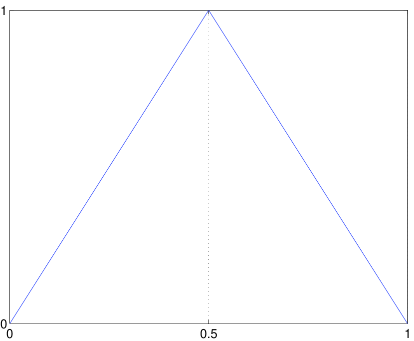
a) the Tent map
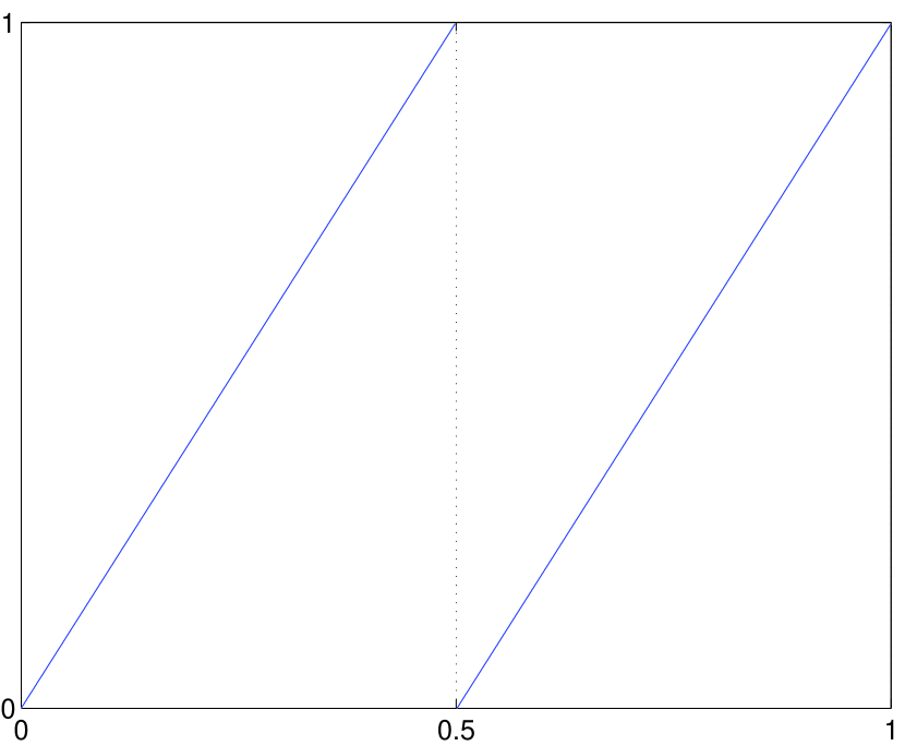
b) the Bernoulli shift map
As we know, the two simple chaotic maps have typical chaotic dynamics [1, 6]: 1) positive Lyaponuv exponents; 2) ergodicity, mixing and exactness; 3) uniform invariant density function ; 4) the Tent map’s auto-correlation function , and the Bernoulli shift map’s auto-correlation function approaches to zero exponentially as . The third property means that the chaotic orbit starting from almost everywhere will lead to the same uniform distribution over the definition interval [0,1]. However, as shown below, this paper points out that such a good dynamics cannot be exhibited in digital computers well, due to the finite-precision effect.
4 Chaotic Maps under Floating-Point Arithmetic
Firstly, assume the initial condition , where (the least significant 1-bit) and . Then, the iteration of the Tent map will be
| (5) |
where denotes the left bit-shifting operation. Note that when . Apparently, after iterations, . Then, , and . That is, the number of required iterations to converge to zero is . Note that when .
For the Bernoulli shift map, we can similarly get
| (6) |
Apparently, after iterations, . That is, the number of required iterations to converge to zero is . Note that when .
From the above analysis, it is clear that no any quantization error is introduced in the digital chaotic iterations, which is because the chaotic iterations can be exactly carried out with the digital operation .
In the following, let us consider the value of in two different conditions of :
-
•
is a normalized number: from Eq. (1), . Assuming the least 1-bit of is , one can immediately get and deduce . Considering and , .
-
•
is a non-zero denormalized number: from Eq. (2), . Assuming the least 1-bit of is , one can immediately get and deduce . Considering , .
To sum up, in both conditions .
In the following, we will prove that the mathematical expectation of is only about much smaller than 1074 if distributes uniformly in the space of all valid floating-point numbers in [0,1]. That is, the mathematical expectation of is much smaller than 1074 for the Bernoulli shift map, and smaller than 1075 for the Tent map.
Firstly, let us consider the mathematical expectation of . Without loss of generality, for a denormalized number or a normalized number with a fixed exponent , assume the mantissa fraction distributes uniformly over the discrete set . Then, the probability that is , and the probability that is . Then, the mathematical expectation of is
| (7) |
Then, let us consider the mathematical expectation of . From the uniform distribution of in the interval [0,1], one has the probability of the exponent is is about . Thus, the mathematical expectation of is
| (8) |
From the above deductions, we can immediately deduce
Generally denormalized numbers will not be used by most pseudo-random number generators, such as the embedded rand function in almost all programming languages, so . That is, for the Bernoulli shift map, and for the Tent map, where means that is much smaller than .
5 Experiments
To verify the analysis given in the last section, a larger number of floating-point numbers are tested for the two maps. Taking the Tent map as an example, the results of three typical numbers, the minimal denormalized number , and a normalized number are given in Figs. 2 and 3, respectively.
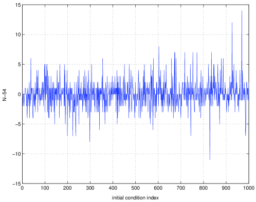
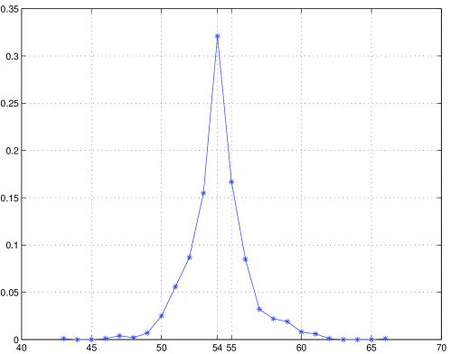
To verify the mathematical expectation of , some experiments are made for test on 1000 initial conditions pseudo-randomly generated with the standard rand function of matlab. The values of corresponding to the 1000 initial conditions are shown in Fig. 4, and the occurrence frequency of different values is shown in Fig. 5. Following the data, we can get the average of is about , which agrees with the theoretical result well.
6 Conclusions
This paper studies the digital iterations of the two well-known chaotic discrete-time maps – the Tent map and the Bernoulli shift map. It is found that all chaotic orbits will be eventually converge to zero within iterations, and that the value of is uniquely determined by the details of digital floating-point arithmetic. Although the given results are rather simple from a computer scientist’s point of view, they really touches the subtle kernel of digital chaos (i.e., chaos in computers).
References
- [1] Shujun Li. Analyses and New Designs of Digital Chaotic Ciphers. PhD thesis, School of Electronic and Information Engineering, Xi’an Jiaotong University, Xi’an, China, June 2003. available online at http://www.hooklee.com/pub.html.
- [2] Dean J. Driebe. Fully Chaotic Maps and Broken Time Symmetry, volume 4 of Nonlinear Phenomena and Complex Systems. Kluwer Academic Publishers, Dordrecht, The Netherlands, 1999.
- [3] Robert L. Devaney. A First Course in Chaotic Dynamical Systems: Theory and Experiment. Addison-Wesley Publishing Company, Inc., Reading, Massachusetts, 1992.
- [4] IEEE Computer Society. IEEE standard for binary floating-point arithmetic. ANSI/IEEE Std. 754-1985, August 1985.
- [5] Steve Hollasch. IEEE standard 754 floating point numbers. online document at http://stevehollasch.com/cgindex/coding/ieeefloat.html, February 2005.
- [6] A. Baranovsky and D. Daems. Design of one-dimensional chaotic maps with prescribed statistical properties. Int. J. Bifurcation and Chaos, 5(6):1585–1598, 1995.