Slowdown and Splitting of Gap Solitons in Apodized Bragg Gratings

Abstract

We study the motion of gap solitons in two models of apodized nonlinear fiber Bragg gratings (BGs), with the local reflectivity $\kappa$ varying along the fiber. A single step of $\kappa$, and a periodic array of alternating steps with opposite signs (a “Bragg superstructure”) are considered. These structures may be used in the design of various optical elements employing the gap solitons. A challenging possibility is to slow down and eventually halt the soliton by passing it through the step of increasing reflectivity, thus capturing a pulse of standing light. First, we develop an analytical approach, assuming adiabatic evolution of the soliton, and making use of the energy conservation and balance equation for the momentum. Comparison with simulations shows that the analytical approximation is quite accurate, unless the inhomogeneity is too narrow, or the step is too high: the soliton is either transmitted across the step or bounces back from it. If the step is narrow, systematic simulations demontrate that the soliton splits into transmitted and reflected pulses (splitting of a BG soliton which hits a chirped grating was observed in experiments). Moving through the periodic “superstructure” , the soliton accummulates distortion and suffers radiation loss if the structure is composed of narrow steps. The soliton moves without any loss or irrieversible deformation through the array of sufficiently broad steps.

I Introduction

Bragg gratings (BGs) are periodic structures produced by a periodic variation of the refractive index along a fiber or an optical waveguide. Devices based on fiber gratings are widely used in optical systems Kashyap . Gap solitons (in this context, they are also called BG solitons Sterke ) are supported by fiber gratings through the balance between the BG-induced linear dispersion (which includes a gap in the system’s linear spectrum) and Kerr nonlinearity of the fiber material. Analytical solutions for BG solitons in the standard fiber-grating model are well known Aceves ; Demetri . Studies of the stability of these solutions have led to a conclusion that almost exactly half of them are stable (see details below) Tasgal . These solitons were created and studied in detail in the experiment experiment ; slowest .

Recently, much attention has been attracted to the creation of “slow light” in various media slowlight , including fibers (for instance, a thin fiber embedded in an electromagnetically controlled molecular solid slowlightJModPhys ). In particular, the possibilities to generate slowly moving optical solitons were considered in various settings slowsoliton ; we_collision . The nonlinear fiber grating is a medium where it may be possible to stop a soliton. Indeed, solutions for zero-velocity gap solitons are available, in which the counter-propagating waves are mutually locked in the dynamical equilibrium between the linear Bragg-resonant conversion and Kerr nonlinearity keeping them together through the XPM (cross-phase-modulation) interaction Aceves ; Demetri .

Actually, the BG solitons that were created in the experiments to date were fast ones, the slowest among them having the velocity equal to half of the light velocity $\overline{c}$ in the fiber slowest . A possibility to capture a standing BG soliton is to bind it on an attractive local inhomogeneity Weinstein ; we (earlier, it was demonstrated that a local defect in the fiber grating can also stimulate a nonlinear four-wave interaction without formation of a soliton trapping ). Moreover, it is possible to combine the attractive inhomogeneity and local linear gain, which is a way to create a permanently pinned soliton in the presence of loss we2 . Stable pinned-solitons are not only objects of fundamental interest, but they also have an obvious potential for design of various nonlinear-optical elements.

Another approach to the creation of standing BG solitons was explored in a recent work we_collision , where it was demonstrated that head-on collisions between two moving solitons may lead to their fusion into an immobile soliton (with residual internal oscillations, which is explained by the existence of an oscillatory intrinsic mode in the stable BG soliton Tasgal ), provided that their initial velocities are smaller than $\approx 0.2~{}\overline{c}$. Thus, one should still bridge the remaining gap between the experimentally available minimum soliton velocity, $0.5\overline{c}$, and the necessary value of $0.2\overline{c}$.

A possibility to resolve this problem was also proposed and briefly considered in Ref. we_collision (a similar possibility was mentioned still earlier in Ref. express ): passing the BG soliton through an apodized fiber grating, with the Bragg reflectivity gradually increasing along the fiber. In this case, the soliton may be adiabatically slowed down. An objective of the present work is to consider this problem in a systematic form, both analytically and numerically. Besides that, we also aim to study the motion of the soliton through a periodic array of alternating reflectivity steps with opposite signs.

It should be mentioned that apodized fiber gratings (a gradually varying reflectivity may also be featured by chirped gratings express ; Tsoy ) are widely used in various applications Kashyap . Some experimental slowest ; express and theoretical Tsoy results concerning passage of BG solitons through apodized gratings were reported earlier. These include the use of the apodization to facilitate the launch of solitons into the fiber grating slowest , observation of splitting of a BG soliton which hits a chirped grating express , and analysis of the soliton’s dynamics in the case when the apodized-grating model reduces to a perturbed nonlinear Schrödinger equation Tsoy . The formulation of problems considered in this work, and methods developed for the analysis, are essentially different from the earlier works, as will be seen below.

The rest of the paper is organized as follows. The model is formulated in section 2, and in section 3 we work out the analytical approach, which is based on treating the gap soliton moving in the apodized BG as a quasi-particle obeying an equation of motion derived from the balance equation for the soliton’s momentum. This adiabatic approach is relevant when the Bragg reflectivity varies on a spatial scale which exceeds the size of the soliton (for slow solitons, a physically relevant size is, typically, $\sim 1$ mm, while for fast solitons the size is additionally subject to the “Lorentz contraction”, see below). Results of systematic numerical simulations of the full model with a step of the Bragg reflectivity (that will also be sometimes called “barrier” ) are presented in section 4. First, we compare the analytical predictions produced by the adiabatic approximation with numerical results, and conclude that the adiabatic approximation is quite accurate, provided that the step is not too steep. Further, we present numerical results for the case of steeper apodization. In that case, the soliton impinging upon the step may split into two secondary solitons (transmitted and reflected ones), or get completely destroyed. In section 5 we briefly describe results of simulations of the motion of the soliton through a periodic array of alternating positive and negative steps. It is found that the soliton distorts itself and emits radiation if the steps are narrow. If they are broader, the deformation of the moving soliton accumulates slower, and it can move without any irreversible damage through the array of sufficiently broad steps. Section 6 concludes the paper.

II The model

The commonly adopted model of the nonlinear fiber grating is based on a system of coupled equations for the local amplitudes of the right- ($u$) and left- ($v$) traveling waves Sterke ,

$$iu_{t}+iu_{x}+\kappa v+\left(|u|^{2}/2+|v|^{2}\right)u = 0,$$

$$iv_{t}-iv_{x}+\kappa u+\left(|v|^{2}/2+|u|^{2}\right)v = 0,$$ (1)

where $x$ and $t$ are the coordinate and time, which are scaled so that the linear group velocity of light in the fiber is $1$, and $\kappa$ is the Bragg-reflectivity coefficient. In the apodized grating, $\kappa$ is a function of $x$.

Exact solutions to Eqs. (1) with $\kappa\equiv\mathrm{const}$, which describe solitons moving at a velocity $c$ ($c^{2}<1$) through the uniform BG, were found in Refs. Aceves and Demetri :

$$u_{\mathrm{sol}} = \sqrt{\frac{2\kappa\left(1+c\right)}{3-c^{2}}}\left(1-c^{2}\right)^{1/4}W(X)\mathrm{exp}\,\left[i\phi(X)-iT\cos\theta\right],$$

$$v_{\mathrm{sol}} = -\sqrt{\frac{2\kappa\left(1-c\right)}{3-c^{2}}}\left(1-c^{2}\right)^{1/4}W^{\ast}(X)\mathrm{exp}\,\left[i\phi(X)-iT\cos\theta\right].$$ (2)

Here, the asterisk stands for the complex conjugation, $\theta$ is an intrinsic parameter of the soliton family which takes values $0<\theta<\pi$, and

$$X = \kappa\left(1-c^{2}\right)^{-1/2}\left[x-\xi(t)\right],\,T=\kappa\left(1-c^{2}\right)^{-1/2}\left(t-cx\right),$$

$$\phi(X) = \frac{4c}{3-c^{2}}\mathrm{\tan}^{-1}\left\{\tanh\left[(\sin\,\theta)X\right]\tan\left(\theta/2\right)\right\},$$ (3)

$$W(X) = \left(\sin\,\theta\right)\,\mathrm{sech}\left[(\sin\,\theta)X-i\left(\theta/2\right)\right]\,,$$

where $d\xi/dt=c$ (note the above-mentioned “ Lorentz contraction” of the soliton’s size, obvious in the definition of $X$).

Equations (1) conserve three dynamical invariants: the norm (frequently called energy in optics) and momentum,

$$E\equiv\int_{-\infty}^{-\infty}\left(\left|u\right|^{2}+\left|v\right|^{2}\right)dx,~{}P=i\int_{-\infty}^{+\infty}\left(u_{x}^{\ast}u+v_{x}^{\ast}v\right)dx,$$ (4)

and also the Hamiltonian (which will not be used below). For the soliton solution (2), the norm and momentum take values

$$E_{\mathrm{sol}} \equiv \frac{8\theta\left(1-c^{2}\right)}{3-c^{2}},$$

$$P_{\mathrm{sol}} = 8\kappa c\sqrt{1-c^{2}}\left[\frac{\left(7-c^{2}\right)}{\left(3-c^{2}\right)^{2}}\left(\sin\theta-\theta\cos\theta\right)+\frac{\theta\cos\theta}{3-c^{2}}\right]$$ (5)

(note that the energy does not depend on $\kappa$).

The expression for the momentum strongly simplifies in the “nonrelativistic” limit ($c^{2}\ll 1$), which makes it possible to identify an effective soliton’s mass,

$$M_{\mathrm{sol}}\equiv\lim_{c\rightarrow 0}\frac{P_{\mathrm{sol}}}{c}=\frac{8\kappa}{9}\left(7\sin\theta-4\theta\cos\theta\right).$$ (6)

Note that the gap solitons are stable in the region $\theta\leq\theta_{\mathrm{cr}}$, where $\theta_{\mathrm{cr}}$ is very close to $\pi/2$ [for instance, $\theta_{\mathrm{cr}}\approx 1.01\left(\pi/2\right)$ if $c=0$] Tasgal . In all the stability region, the mass (6) increases with $\theta$, i.e., larger $\theta$ corresponds to a “heavier” soliton.

III The adiabatic approximation

In the apodized BG, with $\kappa=\kappa(x)$, the momentum is no longer conserved; instead, the following exact equation can be derived from the underlying equations (1):

$$\frac{dP}{dt}=2\int_{-\infty}^{+\infty}\frac{d\kappa}{dx}\mathrm{Re}\left(uv^{\ast}\right)dx.$$ (7)

The adiabatic approximation applies to the case of a slowly changing $\kappa(x)$, when it varies on a length which is essentially larger than the soliton’s size. As it follows from the expressions (3) for the soliton solution, this implies a general condition, $\sin\theta\gg\sqrt{1-c^{2}}\left(\kappa^{-1}\left|d\kappa/dx\right|\right)$.

For slowly varying $\kappa(x)$, we rewrite Eq. (7) as

$$\frac{dP}{dt}=2\frac{d\kappa}{dx}\int_{-\infty}^{+\infty}\mathrm{Re}\left(uv^{\ast}\right)dx,$$ (8)

assuming that the value of $d\kappa/dx$ is taken at the point $x=\xi(t)$, where the soliton’s center is located at a given moment of time, see Eqs. (3). Then, the left-hand side of Eq. (8) can be calculated with the unperturbed soliton solution (2), and the expression for the soliton’s momentum from Eqs. (5) can be substituted in the left-hand side. This yields the following general evolution equation for the soliton’s parameters [the velocity $c(t)$ and the mass parameter $\theta(t)$]:

$$\frac{d}{dt}\left\{\kappa(\xi)c\sqrt{1-c^{2}}\left[\frac{\left(7-c^{2}\right)}{\left(3-c^{2}\right)^{2}}\left(\sin\theta-\theta\cos\theta\right)+\frac{\theta\cos\theta}{3-c^{2}}\right]\right\}$$ (9)

$$= -\frac{d\kappa}{d\xi}\frac{\left(1-c^{2}\right)^{3/2}}{3-c^{2}}\sin\theta.$$

Note that, as $\kappa(x)$ is taken at the point $x=\xi(t)$, which changes in time according to $d\xi/dt=c$, the coefficient $\kappa$ is subject to the $t$-differentiation on the left-hand side of Eq. (9).

Unlike the momentum, the energy of the wave fields remains the dynamical invariant in the presence of the apodization. Therefore, using the expression for the soliton’s energy from Eqs. (5), in the adiabatic approximation one can eliminate $\theta(t)$ in favor of $c(t)$:

$$\theta=\frac{3-c^{2}}{1-c^{2}}\frac{E}{8}.$$ (10)

Thus, Eqs. (9) and (10), together with the above-mentioned relations $\kappa=\kappa(\xi)$ and $d\xi/dt=c$, constitute a closed system of the evolution equations for $\theta(t)$ and $c(t)$.

The adiabatic approximation strongly simplifies in the above-mentioned “nonrelativistic” limit, $c^{2}\ll 1$: Eq. (10) then amounts to $\theta=\mathrm{const}$, the remaining equation for $c(t)$ being

$$\frac{d}{dt}\left(\kappa c\right)=-\frac{3\sin\theta}{7\sin\theta-4\theta\cos\theta}\frac{d\kappa}{d\xi}.$$ (11)

Further, using the identities $d\left(\kappa c\right)/dt\equiv\left[d\left(\kappa c\right)/d\xi\right]\left(d\xi/dt\right)=cd\left(\kappa c\right)/dx\$(as $d\xi/dt\equiv c$), we transform Eq. (11),

$$c\frac{d\left(\kappa c\right)}{d\xi}=-\frac{3\sin\theta}{7\sin\theta-4\theta\cos\theta}\frac{d\kappa}{d\xi},$$

which can be integrated to yield

$$c^{2}(\xi)=\left(\frac{3\sin\theta}{7\sin\theta-4\theta\cos\theta}+c_{0}^{2}\right)\frac{\kappa_{0}^{2}}{\kappa^{2}(\xi)}-\frac{3\sin\theta}{7\sin\theta-4\theta\cos\theta},$$ (12)

where the subscript $0$ refers to initial values. In particular, Eq. (12) implies that the soliton may be brought to a halt ($c^{2}=0$) at a point $\xi_{\mathrm{halt}}$ where $\kappa^{2}$ attains the value

$$\kappa_{\mathrm{halt}}^{2}=\kappa_{0}^{2}\left[1+c_{0}^{2}\frac{\left(7\sin\theta-4\theta\cos\theta\right)}{3\sin\theta}\right].$$ (13)

Of course, the expression (13) makes sense if $\kappa_{\mathrm{halt}}^{2}$ does not exceed the largest value of $\kappa^{2}$ available in a given apodization profile.

Note that, except for the special case when $\kappa^{2}(\xi)=\kappa_{\mathrm{halt}}^{2}$ is attained at $\xi=\infty$, Eq. (12) predicts that the soliton will not be stuck forever at the halt point $\xi_{\mathrm{\ halt}}$, but will actually bounce back. Indeed, with regard to the relation $c=d\xi/dt$, it follows from Eq. (12) that, around the halt point, the soliton’s law of motion takes the form $\xi_{\mathrm{halt}}-\xi\sim\left(t-t_{\mathrm{halt}}\right)^{2}$, where $t_{\mathrm{halt}}$ is the moment of time at which the velocity $c(t)$ vanishes.

We also notice that, if the soliton passes an apodized region (step) across which $\kappa(x)$ increases, then the final value of the velocity, as given by Eq. (12), increases with $\theta$. This complies with the above conclusion that the soliton is heavier for larger $\theta$: due to the inertia, a heavier object suffers smaller deceleration passing a potential step.

IV Numerical results

The underlying equations (1) were simulated with the step-wise profile of the local reflectivity,

$$\kappa(x)=\kappa_{0}+\frac{1}{2}\Delta\kappa\tanh\left(\frac{x-x_{0}}{w}\right),$$ (14)

where the step’s height $\Delta\kappa$ is positive, and a normalization condition is imposed,

$$\kappa(=+\infty)=\kappa_{0}+\left(\Delta\kappa/2\right)\equiv 1.$$ (15)

The width of the step is $w$, and its center is located at the point $x=x_{0}$. The split-step fast-Fourier-transform method was used to run the simulations.

In the simulations, the gap soliton was launched, as the exact solution (2) with a positive velocity $c_{0}$, from the left edge of the integration domain. Results will be presented, chiefly, for stable solitons, which implies that the initial values of $\theta$ should be taken from the interval $\theta_{0}\leq\pi/2$ (see above). In fact, simulations were also performed for solitons with $\theta>\pi/2$. The results are not drastically different for them (a brief description of this case is also given below); in particular, the passage of the step does not catalyze the onset of the soliton’s instability, which develops on a larger time scale.

IV.1 Verification of the adiabatic approximation

First of all, predictions produced by the above adiabatic approximation were checked for the case of a sufficiently smooth step ($w$ not too small). The checkup was done in two stages. In the lowest approximation, the explicit solution (12), that was derived in the “nonrelativistic” approximation, was used, along with the corresponding condition $\theta=\mathrm{const}$. To obtain a more accurate result at the second stage, the full evolution equation (9), combined with the relation (10), was solved numerically. It was concluded that the adiabatic approximation is quite accurate, as long as the step remains smooth. This can be illustrated by typical results obtained for the soliton with the initial value of its intrinsic parameter $\theta_{0}=\pi/2$ impinging on the step with the width $w=6$.

In this case, the special value of the initial velocity $\left(c_{0}\right)_{\mathrm{halt}}$, which provides for the halt of the soliton in the direct simulations, was sought for at fixed values of $\kappa_{0}$ (the “halt” was realized so that the soliton’s velocity would drop to zero, and after being stuck for a long time, the soliton would then very slowly start to move backward). It was thus found that the numerical values are, for instance,

$$\left(c_{0}\right)_{\mathrm{halt}}\left(\kappa_{0}=0.8\right)=0.45;~{}\left(c_{0}\right)_{\mathrm{halt}}\left(\kappa_{0}=0.5\right)=0.74.$$ (16)

On the other hand, for these values of $c_{0}$ the adiabatic approximation predicts which must be the final values of the reflectivity, $\kappa_{\mathrm{final}}\equiv\kappa_{0}+(1/2)\Delta\kappa$ [see Eq. (14 )], that will halt the soliton. In particular, in the “nonrelativistic” approximation, we simply set $c^{2}=0$ in Eq. (12), which yields

$$\kappa_{\mathrm{final}}^{2}=\kappa_{0}^{2}\left(1+\frac{7\sin\theta-4\theta\cos\theta}{3\sin\theta}c_{0}^{2}\right).$$ (17)

The predicted value of $\kappa_{\mathrm{final}}$ must be compared with $\kappa_{\mathrm{final}}\equiv 1$, which was imposed by the normalization (15) adopted in the full numerical simulations.

The “nonrelativistic” approximation predicts, for the two cases indicated in Eq. (16), $\kappa_{\mathrm{final}}=0.971$ and $0.755$, respectively. The former value is quite close to the exact one, $\kappa_{\mathrm{final}}\equiv 1$. The latter value is not very close to it, but the corresponding initial velocity, $c_{0}=0.74$, does not correspond to the “nonrelativistic” case. On the other hand, the use of the full adiabatically derived equation (9) predicts, for the same two cases, $\kappa_{\mathrm{final}}=1.017$ and $1.023$, respectively.

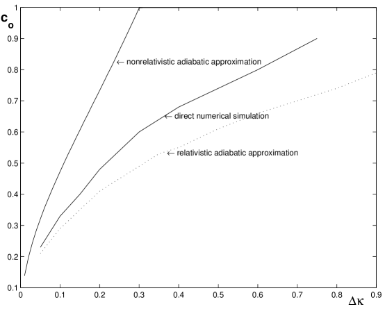
Figure 1: Borders between the bounce of the gap soliton, initially moving at the velocity $c_{0}$, from the local-reflectivity step with the height of $\Delta\kappa$ [see Eq. (14)], and its passage over the step, are shown in the parameter plane $(\Delta\kappa,c_{0})$, as found from direct simulations, and from the analytical approximations – the full (“relativistic”) one, based on Eqs. (9) and (10), and its simplified (“nonrelativistic”) version, which is based on Eq. (12) and assumes $c_{0}^{2}\ll 1$ and $\theta=\mathrm{\ const}$. The results are presented for the fixed step’s width, $w=20$, and fixed mass parameter of the impinging soliton, $\theta=\pi/2$. Both $\Delta\kappa$ and $c_{0}$ are in normalized units.

Systematic comparison of the numerical and analytical results is presented in Fig. 1, which shows the border between the reflection of the moving gap soliton from the apodization step, and its passage through the step, in the plane of ($c_{0}$,$\Delta\kappa$). For smaller values of the step’s size, the analytical approximation provides for results which are quite close to the numerical findings. Making the perturbation stronger (increasing $\Delta\kappa$), we observe a growing deviation, but the full “relativistic” approximation, based on Eqs. (9) and (10), still provides for a reasonable approximation even for larger $\Delta\kappa$ (and larger velocity), while the oversimplified “nonrelativistic” approximation, based on the single equation (12), becomes irrelevant in that case.

IV.2 Different outcomes of the collision of the gap soliton with the apodization step

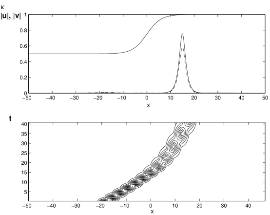
Figure 2: Different typical outcomes of the collision of the gap soliton with the apodization step that has the hight $\Delta\kappa=0.5$ and width $w=6$. The upper panels show the waveforms $|u(x)|$ and $|v(x)|$ (solid and dashed lines) at the end of the simulation, together with the apodization profile, $\kappa(x)$. The lower panels depict the evolution of the field $|u(x)|$ in terms of level contours. (All the variables plotted are in normalized units.) (a) Deceleration of the soliton with very little radiation loss. The initial parameters of the soliton are $c_{0}=0.75$ and $\theta_{0}=0.5\pi$.

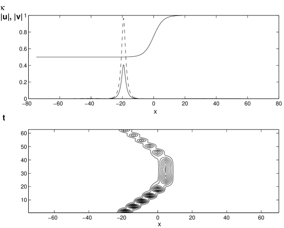
Figure 2: (b) The soliton bouncing back with almost no radiation loss. Here, $c_{0}=0.70$ and $\theta_{0}=0.5\pi$.

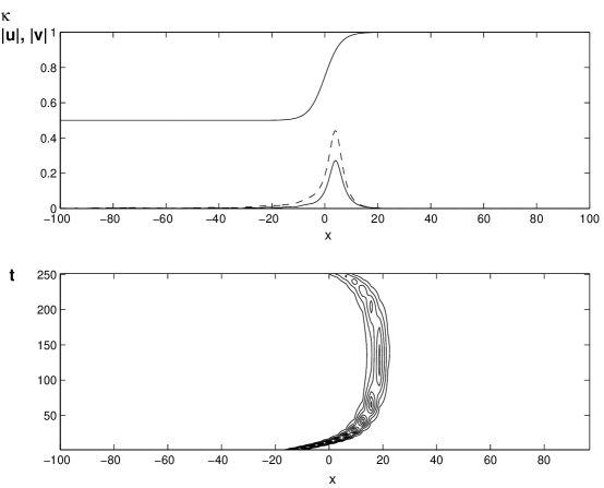
Figure 2: (c) An example of the soliton being halted by the step and staying immobile for a long time. In this case, $c_{0}=0.7403$ and $\theta_{0}=0.5\pi$.

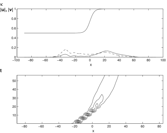
Figure 2: (d) Split of the soliton into two pulses, transmitted and reflected ones. In the course of subsequent evolution, both pulses gradually decay into radiation. In this case, $c_{0}=0.8$ and $\theta_{0}=0.3\pi$.

To present direct numerical results in a systematic form (especially, for the situation with a steeper apodization profile), we first fix the height and width of  the step, setting $\Delta\kappa=0.5$ and $w=6$ [note that this width is much smaller than it was in the case of Fig. 1 ($w=20$), hence the step is much steeper in the present case]. Launching the solitons with various initial values $c_{0}$ and $\theta_{0}$ of the velocity and mass parameter to hit the apodization step, it was found that, as it might be naturally expected, more energetic solitons, with a large velocity $c$ and/or larger mass parameter $\theta$, pass the step with deceleration, a typical example of which is shown in Fig. 2(a), and slower (smaller $c$) and/or lighter (smaller $\theta$) solitons bounce back from the step, see a typical example in Fig. 2(b). Note that the only difference between the cases displayed in Figs. 2(a) and 2(b) is that $c_{0}=0.75$ in the former case, and $c_{0}=0.7$ in the latter case, showing that the border between the transmission and repulsion is in between these values. On the other hand, the calculation based on the quasi-particle equation of motion (9) predicts that the border is at $c=c_{0}\approx 0.61$ for the same case, which agrees reasonably well with the numerical results, considering that the apodization profile is rather steep, and the apodization step is high. The applicability of the adiabatic approximation to the present cases is also corroborated by the observation that very little radiation loss was generated in the direct simulations.

If the bounce takes place at a point $\xi_{\mathrm{halt}}$ located far to the right from the step, the soliton gets stuck there for a finite but long time, also in agreement with the prediction of the quasi-particle approximation. An example of such a case (which, obviously, is of special interest to the experiment and applications, suggesting a real possibility to capture a pulse of “standing light”) is shown in Fig. 2(c). Note that, in comparison with a more generic case of the ricochet shown in Fig. 2(b), in the case of the quasi-trapping of the gap soliton, the bounce indeed occurs after the soliton has advanced much farther to the right.

In the same situation as considered above, but with smaller values of $\theta_{0}$, the quasi-particle approximation does not apply, as the soliton size becomes much larger than the step’s width, hence the step may not be considered as a smooth one in any approximation. The simulations indeed produce a drastically different result in this case: hitting the step, the soliton splits into two pulses, transmitted and reflected ones, which is illustrated by Fig. 2(d). In this case, both pulses eventually decay into radiation, rather than self-trapping into small-amplitude solitons.

The controllable splitting of the incident soliton is an interesting effect in its own right, and it has a potential for various applications. Splitting of the BG soliton hitting a chirped fiber grating has already been observed experimentally and reproduced in numerical simulations express . In fact, in that case the incident soliton split into three pulses: a transmitted soliton and two reflected ones.

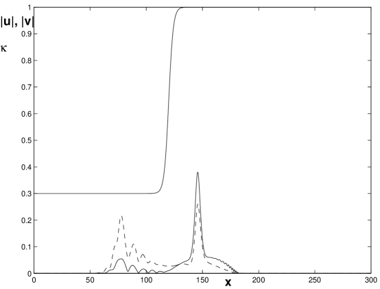
Figure 3: The same as in Fig. 2(d), in the case of a narrower and taller apodization step, with $w=4$ and $\Delta\kappa=0.7$, for the impinging soliton whose mass parameter exceeds the instability threshold, $\theta=0.6\pi$. All the variables plotted are in normalized units.

In this connection, it is relevant to mention that, although we do not display detailed results for the (generally) unstable solitons with $\theta>\pi/2$, the interaction with the step was simulated for them too. In most cases, the intrinsic instability of the soliton does not set it in the course of the limited time before it hits the step (which corresponds to the experimental situation, in which the segment of the fiber grating before the apodized region is not going to be very long experiment ). Then, if the step is smooth, the heavy soliton passes it or bounces back, without catalyzing the onset of the intrinsic instability, and without conspicuous emission of radiation. The soliton emits an appreciable amount of radiation if the barrier is steeper. The splitting of the soliton with $\theta>\pi/2$ into forward and backward moving parts, similar to what is shown for smaller $\theta$ in Fig. 2(d), does not occur on the barrier with $w=6$, which is the value selected for Fig. 2, suggesting that the soliton is a more cohesive object for larger $\theta$ (see further discussion of this point below). Splitting takes place if the barrier is made still steeper and taller – for instance, with $w=4$ and $\Delta\kappa=0.7$, see Fig. 3. As well as in the case displayed in Fig. 2(d), in the latter case the two pulses do not eventually self-trap into secondary solitons, but rather decay into radiation.

IV.3 Scanning the parameter space

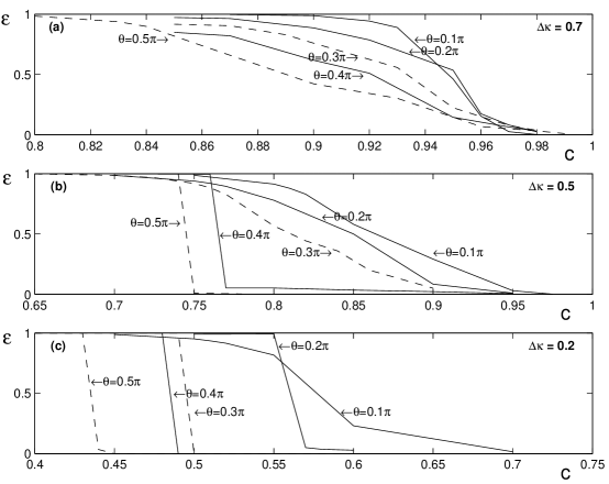
Figure 4: The share of the initial soliton’s energy, which is reflected back by the apodization step of the width $w=6$, versus the initial velocity $c$, for different values of the initial mass parameter $\theta$, and different values of the step’s height $\Delta\kappa$. Three panels of the figure show the dependence $\varepsilon(c)$ in different regions of $c$ and on different scales, in order to highlight regions where nontrivial changes occur. The steep drop of $\varepsilon$ from $1$ to $0$ for larger $\theta$ (such as $\theta=0.4$ and $0.5$) implies the transition from the bounce of the soliton to the transmission without splitting. ($\varepsilon$ is dimensionless, and $c$ is in normalized unit.)

Having displayed typical examples of different outcomes of the collision, we proceed to summarize the results in a systematic form. First, a comprehensive description of the transition from the bounce of the soliton to the passage, together with the splitting (if any), are provided, for different values of the barrier’s height $\Delta\kappa$, by the plots in Fig. 4. For fixed $\theta$, they show the share $\varepsilon$ of the initial soliton’s energy which is reflected back as a result of the interaction of the soliton with the step. A steep drop from $\varepsilon=1$ to $\varepsilon=0$ in Figs. 4(b) and 4(c) implies the transition from the bounce to the transmission without splitting. On the contrary, a gentle crossover means that the impinging soliton was split into two parts, with the energy ratio between them depending on the initial velocity. These plots clearly show strengthening of the soliton’s integrity (its stabilization against the splitting) with the increase of its energy.

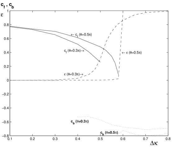
Figure 5: The final velocity $c_{f}$ of the transmitted pulse and the velocity $c_{b}$ of the reflected one (solid lines) are shown, together with the backscattered-energy share $\varepsilon$, versus the height of the apodization step $\Delta\kappa$, for $\theta=0.3\pi$ and $\theta=0.5\pi$. The splitting of the incident soliton takes place in the interval where both solid curves are present. In this figure, the step’s width and initial velocity are fixed, $w=6$ and $c_{0}=0.8$. ($\varepsilon$ is dimensionless, and $c_{f}$, $c_{b}$, $\Delta\kappa$ are in normalized units.)

Further, in Fig. 5 we show the velocities $c_{f}$ and $c_{b}$ of the transmitted (“final”) and reflected (bouncing) fragments of the incident soliton, together with the backscattered-energy share $\varepsilon$, as functions of $\Delta\kappa$. In the ranges where only one velocity is shown in Fig. 5, the soliton is transmitted or reflected as a whole, while the splitting takes place in intervals of the values of $\Delta\kappa$ where both continuous curves (for $c_{f}$ and $c_{b}$) coexist in Fig. 5.

Note that the transition from the full transmission to full reflection, i.e., from $\varepsilon=0$ to $\varepsilon=1$, takes place in exactly the same interval where the splitting occurs, cf. Fig. 4. As is seen, the splitting interval is very narrow for the heavier soliton, with $\theta=0.5\pi$, and much broader for the lighter one, with $\theta=0.3\pi$, which is another common feature with the dependences displayed in Fig. 4.

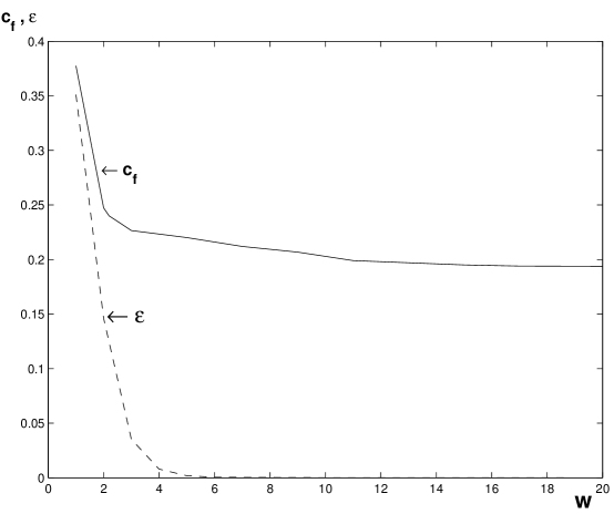
Figure 6: The final soliton’s velocity $c_{f}$ (solid line) and the fraction of the backscattered energy, $\varepsilon$ (dashed line), versus the apodized-layer’s width $w$, in the case when the height of the step is $\Delta\kappa=0.5$. In this figure, the initial velocity and mass parameter of the soliton are fixed to be $c_{0}=0.75$ and $\theta_{0}=0.5\pi$. ($\varepsilon$ is dimensionless, and $c_{f}$, $w$ are in normalized units.)

The dependence of the outcome of the collision on the width of the apodization region was studied too, as it helps to understand how really wide the barrier must be to secure the adiabatic character of the interaction, and how narrow it is when the splitting occurs. In Fig. 6, we show the dependence of the final velocity of the transmitted soliton, $c_{f}$, and the reflected-energy share, $\varepsilon$, on the width while the step’s height is fixed, $\Delta\kappa=0.5$. The final velocity of the transmitted soliton approaches an asymptotic value for large values of $w$.

Figure 6 shows that the transition from the strongly non-adiabatic regime (with splitting) to a nearly adiabatic one is steep itself, taking place in a relatively narrow interval around $w=3$. A practically important implication of the results presented in Fig. 6 is that, for the experimentally relevant case, with the intrinsic size of the BG soliton $\sim 1$ mm experiment , the step which may be regarded as a sufficiently smooth one should have the width ${}_{\sim}^{>}~{}3$ mm.

V Dynamics of the gap soliton in a periodically-apodized structure

To test the robustness of the gap solitons in the fiber gratings with a variable Bragg reflectivity $\kappa$, and its potential for the use in more sophisticated devices, we also simulated the motion of the soliton in the grating subjected to a periodic modulation of $\kappa$. It was built as a periodic concatenation of steps with alternating signs of $\Delta\kappa$; the fiber grating of this type may be considered as a Bragg “superstructure”. This scheme can be realized either directly in a long periodically modulated grating, or as an apodized BG written in a fiber loop, although the stability problems in these two settings are not equivalent. The soliton dynamics in such a superstructure is a problem of interest in its own right – cf. the study of solitons in other periodic strongly inhomogeneous nonlinear optical media, such as fibers with dispersion management DM , various schemes with “nonlinearity management” nonlin_management (including layered media with a periodically changing sign of the Kerr nonlinearity layered ), “tandem” structures tandem , the “split-step” model SSM , waveguide-antiwaveguide concatenations Gisin , etc. A unifying feature of these systems is the surprising robustness of the solitons in them.

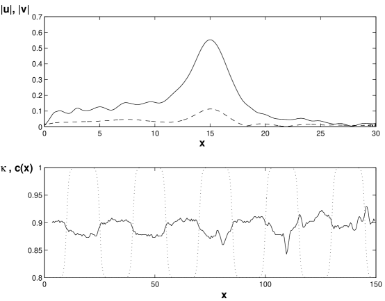
Figure 7: Motion of the soliton with the initial velocity $c_{0}=0.9$ and initial mass parameter $\theta_{0}=0.5\pi$ through a periodic structure consisting of alternating steps with the local Bragg reflectivity $\kappa$ varying between $0.8$ and $1$. Bottom portions in each panel show the profile of $\kappa(x)$ (dotted line) and evolution of the soliton’s velocity (continuous line). The top portions show the shape of the soliton ($|u(x)|$ and $|v(x)|$) at the end of the long simulation. (All the variables plotted are in normalized units.) (a): The width of the individual step is $w=1$ (a non-adiabatic case).

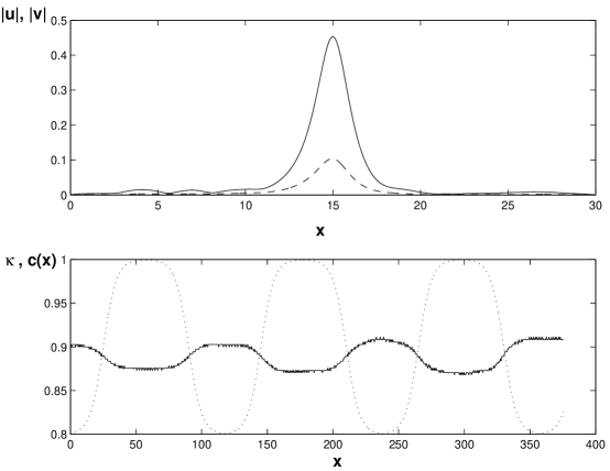
Figure 7: (b): The width of each step is $w=10$ (a nearly adiabatic case).

Typical results produced by the simulations of the soliton propagation in the periodic “superstructure” are displayed in Fig. 7. It can be seen that the soliton travels slower in segments with larger $\kappa$, and faster in those with smaller $\kappa$. In the case when the width $w$ of each step is relatively small [for instance, $w=1$, see panel 7(a)], the soliton evolution is clearly non-adiabatic, cf. the above results for the single step (we stress that the full modulation period in the present case is essentially large than $w$, see Fig. 7). Accordingly, the soliton gradually develops distortions in its shape and simultaneously emits radiation waves. Parallel to distorting itself, the soliton also develops random fluctuations of its velocity.

In the case when the periodic structure is composed of steps with a larger width, for instance, $w=10$ [see Fig. 7(b)], the soliton also accumulates distortion and generates some radiation loss, but, in accordance with the expectation that the evolution must be close to adiabatic in this case, this happens much slower, and the distortion remains mild after passing a long distance. With a still larger step width (for instance, $w=15$), no accumulation of distortion or radiation could be seen at all (the latter case is not shown here, as one would simply observe an unperturbed soliton). So, large values of $w$ indeed provide for the adiabatic character of the soliton’s motion through the periodic structure, but the smallest size of $w$ which makes it possible in the case of the periodic system is (quite naturally) much larger than the minimum width which provided for the adiabatic passage of the gap soliton through the single step, cf. Fig. 6.

Lastly, it is relevant to mention that virtually identical results were observed in the simulations of the periodic system either with periodic boundary conditions (b.c.) in $x$ (which corresponds to the above-mentioned case of an apodized BG written in a fiber loop) or just in a long domain with absorbing b.c. Thus, the same soliton dynamics is expected in both above-mentioned physical realizations of the periodic “Bragg superstructure”.

VI Conclusion

In this work, we have studied in detail motion of gap solitons in two models of apodized fiber Bragg gratings, including, respectively, a single step of the local reflectivity, or a periodic “Bragg superstructure” consisting of alternating steps with opposite signs. Both structures offer a potential for the design of various optical elements employing the gap (Bragg) solitons. The most important implication of the considered problem is a possibility to halt the soliton by passing it through a step with an increasing reflectivity, and eventually to capture a pulse of standing light.

We have developed an analytical approach, which assumes adiabatic evolution of the soliton, and is based on the balance equation for its momentum and conservation of the energy. The result of the analysis can be obtained in a fully explicit form in the “nonrelativistic” case, and in an implicit form (as an ordinary differential equation) in the general case. Comparison of the predictions produced by the approximation with direct simulations shows good accuracy, provided that the width of the inhomogeneity is essentially larger than the soliton’s intrinsic width.

Results of systematic direct simulations of the soliton’s motion were summarized, showing that the soliton is either transmitted across the step or bounces from it, provided that the step is not too narrow; in particular, it is possible to halt the soliton for a very long time. If the step is narrow (so that the interaction of the incident soliton with it is no longer adiabatic), the soliton may split into two pulses, transmitted and reflected ones (the splitting of a gap soliton in a chirped fiber grating has already been observed in the experiment express ). We have studied in detail dependences of the outcome of the interaction on the height and width of the step, as well as on the initial parameters (velocity and effective mass) of the soliton. In particular, a general conclusion is that the soliton is a more cohesive object, being less prone to the splitting, if its energy (effective mass) is larger.

Moving across the periodic structure, the soliton accumulates distortion and radiation loss if the structure is composed of narrow steps. The perturbations accumulate much slower if the steps are wider, and in the system composed of sufficiently wide steps the soliton can move without any loss or irreversible deformation.

Figures

References

- (1) R. Kashyap. Fiber Bragg gratings (Academic Press: San Diego, 1999).
- (2) C.M. de Sterke and J.E. Sipe, Progr. Opt. 33, 203(1994).
- (3) A.B. Aceves and S. Wabnitz, Phys. Lett. A 141, 37(1989).
- (4) D.N. Christodoulides and R.I. Joseph, Phys. Rev. Lett. 62, 1746 (1989).
- (5) B.A. Malomed and R.S. Tasgal, Phys. Rev. E 49, 5787 (1994); I..V. Barashenkov, D.E. Pelinovsky, and E.V. Zemlyanaya, Phys. Rev. Lett. 80, 5117-5120 (1998); A. De Rossi, C. Conti, and S. Trillo, Phys. Rev. Lett. 81, 85 (1998).
- (6) B.J. Eggleton, R.E. Slusher, C.M. de Sterke, P.A. Krug, and J.E. Sipe, Phys. Rev. Lett. 76, 1627 (1996); C.M. de Sterke, B.J. Eggleton, and P.A. Krug, J. Lightwave Technol. 15, 1494 (1997).
- (7) B.J. Eggleton, C.M. de Sterke, and R.E. Slusher, J. Opt. Soc. Am. B 16, 587 (1999).
- (8) J. Marangos, Nature 397, 559 (1999); K.T. McDonald, Am. J. Phys. 68, 293(2000); U. Leonhardt and P. Piwnicki, J. Mod. Optics 48, 977 (2001); U. Leonhardt, Nature 415, 406 (2002); E. Cerboneschi, F. Renzoni, and E. Arimondo, Opt. Commun. 208, 125(2002); J. Opt. B 4, S267 (2002); E. Paspalakis and P.L. Knight, J. Opt. B 4, S372 (2002); A. Godone, F. Levi and S. Micalizio, Phys. Rev. A 66, 043804 (2002); A.D. Wilson-Gordon and H. Friedmann, J. Mod. Optics 49, 125 (2002); M. Xiao, IEEE J. Sel. Top. Quant. Electr. 9, 86 (2003); M.S. Bigelow MS, N.N. Lepeshkin, R.W. Boyd, Phys. Rev. Lett. 90, 113903 (2003); Science 301, 200 (2003); M.O. Scully and M.S. Zubairy, Science 301, 181 (2003); J.N. Munday and W.M. Robertson, Appl. Phys. Lett. 83, 1053 (2003); K. Kim, F. Xiao, C. Lee, S. Kim, X.Z. Chen, and J. Kim, J. Phys. B 36, 2671(2003).
- (9) A.K. Patnaik, J.Q. Liang and K. Hakuta, Phys. Rev. A 66, 063808 (2002); J. Mod. Optics 50, 2595(2003).
- (10) J.E. Heebner, R.W. Boyd, and Q.H. Park, Phys. Rev. E 65, 036619 (2002); C. Conti, G. Assanto and S. Trillo, J. Nonlin. Opt. Phys. Materials 11, 239 (2002).
- (11) W.C.K. Mak, B.A. Malomed, and P.L. Chu, Phys. Rev. E 68, 026609 (2003).
- (12) R.H. Goodman, R.E. Slusher, and M.I. Weinstein, J. Opt. Soc. Am. B 19, 1635(2002).
- (13) W.C.K. Mak, B.A. Malomed, P.L. Chu, J. Opt. Soc. Am. B 20, 725(2003).
- (14) C.M. de Sterke, E.N. Tsoy, and J.E. Sipe, Opt. Lett. 27, 485(2002).
- (15) W.C.K. Mak, B.A. Malomed, and P.L. Chu, Phys. Rev. E 67, 026608 (2003).
- (16) R.E. Slusher, B.J. Eggleton, T.A. Strasser, and M. de Sterke, Optics Express 3, 465 (1998).
- (17) E. Tsoy and C.M. de Sterke, Phys. Rev. E 62, 2882 (2000).
- (18) J.H.B. Nijhof, N.J. Doran, W. Forysiak and F.M. Knox, Electron. Lett. 33, 1726 (1997).
- (19) C. Paré, A. Villeneuve, P.-A. Belangé, and N.J. Doran, Opt. Lett. 21, 459 (1996); C. Paré, A. Villeneuve, and S. LaRochelle, Opt. Commun. 160, 130 (1999); L.J. Qian, X. Liu, and F.W. Wise, Opt. Lett. 24, 166 (1999); X. Liu, L. Qian, and F. Wise, Opt. Lett. 24, 1777 (1999); F.O. Ilday and F.W. Wise, J. Opt. Soc. Am. B 19, 470 (2002); R. Driben, B.A. Malomed, M. Gutin and U. Mahlab, Opt. Commun. 218, 93(2003).
- (20) L. Bergé, V.K. Mezentsev, J. Juul Rasmussen, P.L. Christiansen, and Yu.B. Gaididei, Opt. Lett. 25, 1037 (2000); I. Towers and B.A. Malomed, J. Opt. Soc. Am. B 19, 537 (2002).
- (21) L. Torner, IEEE Photon. Techn. Lett. 11, 1268 (1999); L. Torner, S. Carrasco, J.P. Torres, L.-C. Crasovan, and D. Mihalache, Opt. Commun. 199, 217 (2001).
- (22) R. Driben and B.A. Malomed, Opt. Commun. 185, 439 (2000); ibid. 197, 481 (2001).
- (23) A. Kaplan, B.V. Gisin, and B.A. Malomed, J. Opt. Soc. Am. B 19, 522 (2002).