Origin of the Transition Inside the Desynchronized State in Coupled Chaotic Oscillators

Abstract

We investigate the origin of the transition inside the desynchronization state via phase jumps in coupled chaotic oscillators. We claim that the transition is governed by type-I intermittency in the presence of noise whose characteristic relation is $\langle l\rangle\propto\exp(\alpha|\epsilon_{t}-\epsilon|^{3/2})$ for $\epsilon_{t}-\epsilon<0$ and $\langle l\rangle\propto(\epsilon_{t}-\epsilon)^{-1/2}$ for $\epsilon_{t}-\epsilon>0$, where $\langle l\rangle$ is the average length of the phase locking state and $\epsilon$ is the coupling strength. To justify our claim we obtain analytically the tangent point, the bifurcation point, and the return map which agree well with those of the numerical simulations.

I Introduction

Recently synchronization phenomena in coupled chaotic oscillators have been extensively studied because of their fundamental importance in areas of science and technology such as laser dynamics, electronic circuits, and biological systemsApps ; Tut ; Strogatz . Due to interaction between two coupled chaotic oscillators, various features of synchronization are observed depending on the coupling strength. For example, when two identical chaotic oscillators are coupled, they can be synchronized either perfectlySync or intermittentlyRim . In another case, where they are coupled with slight parameter mismatch, non-synchronization, phase synchronizationPhaseSync1 ; PhaseSync2 ; Rosa , or lag synchronizationLag is observed depending on the coupling strength. Among these features, the noteworthy one of our study is phase synchronization (PS)PhaseSync1 ; PhaseSync2 ; Rosa . As is widely understood, above the critical strength of the coupling for the transition to PS, suitably defined phases of two chaotic oscillators are locked while their amplitudes remain chaotic and uncorrelated. And below the critical value, the phases of two oscillators are intermittently unlocked, that is, $2\pi$ phase jumps interrupt the phase locking states irregularly. So it can be said that the transition from nonsynchronous state to PS state is typically accompanied by an intermittent sequence of $2\pi$ phase jumpsPhaseSync1 ; Lee .

To explain the transition mechanism to PS, two different approaches have been introduced: topologicalPhaseSync1 ; PhaseSync2 ; Rosa and statisticalLee ; IBKim . The topological approach assumes that the behavior of coupled chaotic oscillators is analogous to that of a chaotic oscillator driven by an external chaotic signalTopo . From this study it was concluded that the phase jump phenomenon stems from a boundary crisisFBasin mediated by an unstable-unstable pair bifurcation, which is termed eyelet intermittencyEyelet . Meanwhile, the statistical approach focuses on a phase equation which describes the phase difference of coupled chaotic oscillators. A potential modulated by multiplicative noise was derived by the analysis of the phase equation and it was concluded that the transition mechanism is similar to that of eyelet intermittencyLee .

By taking the statistical approach, however, we are to show in this paper that the characteristic relation of the average length of the phase locking state (or average laminar length) on the coupling strength before the transition to PS in coupled Rössler oscillators follows the relation of type-I intermittency in the presence of noise. To validate our argument, we derive a one-dimensional phase equation from the coupled Rössler oscillators and obtain the bifurcation point, the tangent point that is a $\pi/2$ phase locking state, and the return map analytically, which exactly agree with those of the numerical simulations. And then we obtain the characteristic relations of $\langle l\rangle\sim\exp(\alpha|\epsilon_{t}-\epsilon|^{3/2})$ for $(\epsilon_{t}-\epsilon)<0$ and of $\langle l\rangle\sim(\epsilon_{t}-\epsilon)^{-1/2}$ for $(\epsilon_{t}-\epsilon)>0$ which are the same as those of type-I intermittency in the presence of noiseKye ; Eckman , where $\langle l\rangle$ is the average length of the phase locking state, $\epsilon$ is the coupling strength and $\epsilon_{t}$ is the tangent bifurcation point.

In our approach, the analytic scaling rule is obtained from the Fokker-Planck equation FPE and so it describes the asymptotic behavior near PS regime in which the effective noise can be reasonably approximated to be Gaussian IBKim ; Kye . For this reason, it seems that critical coupling does not appear in our formalism. However in real systems there is one critical coupling $\epsilon_{c}$ which is defined as a border of existence of phase slips, because of a finite amplitude of the effective noise.

In section II, we will obtain phase difference equation of coupled Rössler oscillators from one-dimensional phase equation and compare the analytical and numerical return maps of the phase difference in Section III. After that we will obtain the characteristic relations of intermittent phase locking time according to the coupling strength by Fokker-Planck equation in Section IV, discuss the results in Section V, and conclude our study in Section VI.

II Analytic study of Coupled Rössler Oscillators

The transition to PS was first observed in coupled Rössler oscillators which have a slight parameter mismatch PhaseSync1 ,

$$\dot{x}_{1,2} = -\omega_{1,2}y_{1,2}-z_{1,2}+\epsilon(x_{2,1}-x_{1,2}),$$

$$\dot{y}_{1,2} = \omega_{1,2}x_{1,2}+0.15y_{1,2},$$ (1)

$$\dot{z}_{1,2} = 0.2+z_{1.2}(x_{1,2}-10.0),$$

where $\omega_{1,2}$ $(=1.0\pm 0.015)$ are the overall frequency of each oscillator and $\epsilon$ is the coupling strength. By transforming the above equation to the polar form, we obtain the following one-dimensional phase equation, which describes the phase difference of the two oscillators:

$$\frac{d\phi}{dt}\!=\!\Delta\omega+A(\theta_{1},\theta_{2},\epsilon)\sin\phi+B(\theta_{1},\theta_{2})\epsilon+\xi(\theta_{1},\theta_{2}),$$ (2)

where,

$$A(\theta_{1},\theta_{2},\epsilon) = (\epsilon+0.15)\cos(\theta_{1}+\theta_{2})-\frac{\epsilon}{2}(\frac{R_{2}}{R_{1}}+\frac{R_{1}}{R_{2}}),$$

$$B(\theta_{1},\theta_{2}) = -\frac{1}{2}(\frac{R_{2}}{R_{1}}-\frac{R_{1}}{R_{2}})\sin(\theta_{1}+\theta_{2}),$$

$$\xi(\theta_{1},\theta_{2}) = \frac{z_{1}}{R_{1}}\sin(\theta_{1})-\frac{z_{2}}{R_{2}}\sin(\theta_{2}),$$ (3)

$\Delta\omega=\omega_{1}-\omega_{2}$, $\phi=\theta_{1}-\theta_{2}$, $\theta_{1,2}=\arctan(y_{1,2}/x_{1,2})$, and $R_{1,2}=\sqrt{x_{1,2}^{2}+y_{1,2}^{2}}$. Here $B$, $\xi$, and $(\epsilon+0.15)\cos(\theta_{1}+\theta_{2})$ in $A$ are fast fluctuating terms in comparison with slowly varying $\phi$.

Figure 1: The values of $\langle A\rangle$, $\langle B\rangle$, $\langle\xi\rangle$, $\frac{\Delta\tilde{\omega}}{\langle A\rangle}$, and $\tilde{\epsilon}$ according to the coupling strength: (a) the mean values of A(circle), B(square), and $\xi$(filled circle); (b) and (c) the values of $\frac{\Delta\tilde{\omega}}{\langle A\rangle}$ and $\tilde{\epsilon}$ (the arrows point out the bifurcation point $\epsilon_{t}$).

Whereas, in the previous studies, the authors neglected all of the fast fluctuating termsLee , we found that they play a crucial role in the analysis of the transition mechanism. Equation (2) can be transformed into the following simple form:

$$\frac{d\phi}{dt}=\Delta\tilde{\omega}+\langle A\rangle\sin\phi+\tilde{\xi},$$ (4)

where $\tilde{\xi}=(\xi-\langle\xi\rangle)+(B-\langle B\rangle)\epsilon+(A-\langle A\rangle)\sin\phi$, and $\Delta\tilde{\omega}=\Delta\omega+\langle\xi\rangle+\langle B\rangle\epsilon$. Here $\langle A\rangle$ and $\langle B\rangle$ are the mean value of $A$ and $B$ respectively. This equation is similar to the one describing a phase locking of the periodic oscillator in the presence of noise Stratonovich .

In Eq. (4), if we turn off $\tilde{\xi}$, the analysis of the system stability is straightforward. If $\frac{d\phi}{dt}=0$ the system ends time-evolution and $\phi$ remains at $\phi^{*}$, where

$$\phi^{*}=\arcsin(-\frac{\Delta\tilde{\omega}}{\langle A\rangle}).$$ (5)

Here the condition of $\phi^{*}$ being stable is $|\frac{\Delta\tilde{\omega}}{\langle A\rangle}|\leq 1$. Tangent bifurcation occurs at $\frac{\Delta\tilde{\omega}}{\langle A\rangle}=-1$ and the tangent point is $\phi^{*}_{\pm}=\pm\frac{\pi}{2}\pm 2\pi n$, where $n=0,1,2,...$ and the sign $\pm$ depends on $\Delta\omega$. In our system since $\Delta\omega$ is positive, only $\phi^{*}_{+}$ appears. This explains why $\phi$ is locked near $\pm\frac{\pi}{2}\pm 2\pi n$ and $2\pi$ phase jumps occurPhaseSync1 ; Lee .

III Numerical Study and return maps

If Eq. (4) is expanded around the tangent point $\phi^{*}_{+}$, the following equation is obtained: $\frac{d\tilde{\phi}}{dt}\approx\tilde{\epsilon}+a\tilde{\phi}^{2}+\tilde{\xi}$, where $\tilde{\phi}=\phi-\pi/2$, $\tilde{\epsilon}=\Delta\tilde{\omega}+\langle A\rangle$, and $a=-\langle A\rangle/2$. Here if $\tilde{\xi}$ is absent, $\tilde{\phi}$ moves very slowly around the tangent point $\phi^{*}$. So the dynamics of $\tilde{\phi}$ is mainly governed by $\tilde{\xi}$ in the situation $|\tilde{\xi}|\gg|\tilde{\epsilon}|$. Then we can regard $\tilde{\phi}^{2}$ as a constant when the two oscillators are in a locked state. We obtain a local Poincaré map by integrating the above equation during the period that oscillator 1 completes every N rotation (the structure of the local Poincaré map is invariant with respect to the number of N as far as N is small enough in comparison with the average length of the phase locking state). The local Poincaré map is given by:

$$\phi_{n+1}=\phi_{n}+\tilde{\epsilon}^{\prime}+\tilde{a}\phi_{n}^{2}+\xi_{n},$$ (6)

where $\tilde{\epsilon}^{\prime}=\tilde{\epsilon}\langle T_{n}\rangle$, $\tilde{a}=\frac{1}{2}\langle\int_{\tau_{n-1}}^{\tau_{n}}Adt\rangle$, and $\xi_{n}=\int_{\tau_{n-1}}^{\tau_{n}}\tilde{\xi}dt+\frac{1}{2}(\int_{\tau_{n-1}}^{\tau_{n}}Adt-\langle\int_{\tau_{n-1}}^{\tau_{n}}Adt\rangle)$. Here $T_{n}$ is $\tau_{n}-\tau_{n-1}$, where $\tau_{n}$ is the overall time that oscillator 1 takes to complete $N$ rotations. This is the very local Poincaré map of type-I intermittency in the presence of noiseHirsch when $\xi_{n}$ acts as random noise. In this equation tangent bifurcation occurs at the point $\tilde{\epsilon}^{\prime}=0$, which meets the condition of $\frac{\Delta\tilde{\omega}}{\langle A\rangle}=-1$. To determine the tangent bifurcation point, we calculate $\langle A\rangle$, $\langle B\rangle$, $\langle\xi\rangle$, $\frac{\Delta\tilde{\omega}}{\langle A\rangle}$, and $\tilde{\epsilon}$ according to the coupling strength $\epsilon$ as presented in Fig. 1 (a), (b), and (c), respectively. The figures show that the value of $\epsilon$ at the bifurcation point is $0.0277$.

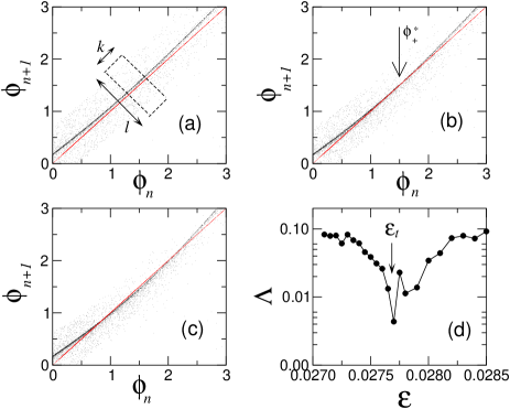
Figure 2: The return maps $(\phi_{n},\phi_{n+1})$ and $N$ as a function of $\epsilon$: (a), (b), and (c) are the return maps before ($\epsilon=0.018$), near ($\epsilon=0.028$), and after ($\epsilon=0.035$) the tangent bifurcation point, respectively; (d) shows that the minimum value of $\Lambda$ appears at $\epsilon_{t}=0.0277$ (when $k=0.03$ and $l=0.6$).

In order to verify the above analytic results, we construct the return maps directly from Eqs. (1)-(3) by obtaining $\phi$ for $N=1$. Figure 2(a), (b), and (c) show the return maps before, near, and after the tangent bifurcation point, respectively. The figures show that as the coupling strength $\epsilon$ increases, the shadow curve approaches the diagonal line. When the curve touches the diagonal line, tangent bifurcation occurs and the tangent point is $\frac{\pi}{2}$ (see the inset arrow in Fig. 2(b)), which agrees well with the one obtained in the above.

We define a measure $\Lambda=|(n_{+}-n_{-})/(n_{+}+n_{-})|$, where $n_{+}$ is the number of points above the diagonal line in the total number of points inside of the rectangle of $k\times l$ and $n_{-}$ is the number of points below the diagonal line. Then the measure shows the average ratio between above and below the passage near the tangent point. So the minimum value of $\Lambda$ indicates the bifurcation point. Figure 2(d) shows a sharp minimum at $\epsilon\approx 0.0277$. This value again agrees with what we obtained from Fig. 1(b) and (c).

The shadow curves are well fitted to the following form of type-I intermittencyPM ; Kim :

$$\hat{\phi}_{n+1}=\hat{\phi}_{n}+\hat{a}\hat{\phi}^{2}_{n}+\hat{\epsilon},$$ (7)

where $\hat{\phi}_{n}=\phi_{n}-\frac{\pi}{2}$, $\hat{a}\approx 0.094$, and $\hat{\epsilon}=\epsilon_{t}-\epsilon$. The coefficient $\hat{a}$ in Eq. (7) agrees well with $\tilde{a}$ in Eq. (6), since $\langle T_{n}\rangle\approx 2\pi$ and the mean value of $A$ is $-0.03$. (The overall frequency $\omega_{1,2}\approx 1.0$.) This confirms that the phase equation of the coupled Rössler oscillators coincide with the structure of type-I intermittency.

IV Result from Fokker-Planck Equation

Under the long laminar length approximation, Eq. (6) can be transformed into the differential form $\frac{d\phi}{dt}=\tilde{\epsilon}^{\prime}+\tilde{a}{\phi}^{2}+\tilde{\xi}$. Then we can obtain the Fokker-Planck equation (FPE) by regarding $\xi_{n}$ as Gaussian white noiseGardiner ; FPE . The probability distribution and auto-correlation of $\xi_{n}$ are examined for various $N$s. So we find they are in better agreement with the Gaussian distribution and $\delta$-correlation, respectively, as $N$ becomes larger. Figure 3 shows the probability distribution and auto-correlation of $\xi_{n}$ for $N=25$ which coincide with the Gaussian profile with a dispersion of $0.4$ and the $\delta$-function, respectively. ($N=25$ is still much less than the average length of the phase locking state that we have obtained.) The noise with the Gaussian distribution is not bounded whereas $\xi_{n}$ in coupled Rössler oscillators is bounded within $(-1.3,1.3)$. However, from the numerical data, we find that the probability of the occurrence of events outside the bounded region of $\xi_{n}$ is less than $1.0\times 10^{-8}\%$. So it is a negligible effect on the average length of the phase locking state.

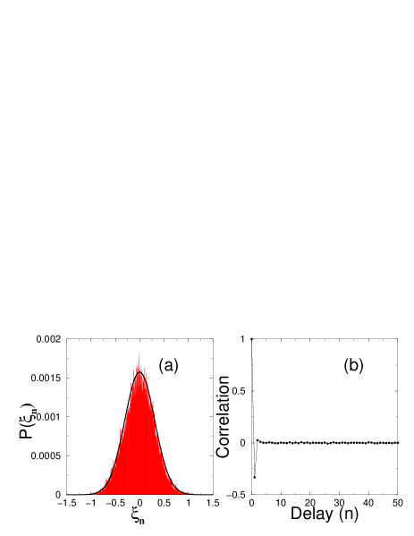
Figure 3: The distribution and auto-correlation of $\xi_{n}$ for $N=25$. (a) the distribution of $\xi_{n}$ well fitted to the Gaussian profile, and (b) the auto-correlation of $\xi_{n}$ almost $\delta$-correlated.

From the FPE with appropriate boundary conditionsKye ; Eckman ; Gardiner ; Hirsch , we can obtain the characteristic form of the average laminar length according to the coupling strength $\epsilon$ as follows:

$$\langle l\rangle\cong\langle l_{0}\rangle\exp(\alpha|\epsilon_{t}-\epsilon|^{3/2}),$$ (8)

where $\alpha$ is the constant and $\langle l_{0}\rangle$ is the average length of the phase locking state at the tangent bifurcation point. Figure 4(a) shows the average length of the phase locking state for $N=1$ as a function of $|\epsilon_{t}-\epsilon|$ in the region $0.0200\leq\epsilon\leq 0.0302$. The slope in the space $\ln|\epsilon_{t}-\epsilon|$ versus $\ln(\ln\langle l\rangle-\ln\langle l_{0}\rangle)$ is $1.44$ as shown in Fig. 4(b) and its inset (c). The line fits well within $4.0$% error from the 3/2 slope. The slope of the tail in Fig. 4 (b) converges to 1 Slope1 which shows the transient regime from $\langle l\rangle\propto(\epsilon_{t}-\epsilon)^{-1/2}$ to $\langle l\rangle\propto\exp(\alpha|\epsilon_{t}-\epsilon|^{3/2})$. Figure 4(d) is the plot of $\ln(\epsilon_{t}-\epsilon)$ versus $\ln\langle l\rangle$ in the region $0.024\leq\epsilon\leq 0.0277$ and the tail also clearly shows the transient regime. The straight line fits well with the $-1/2$ slope. This means that the characteristic relation deforms from the conventional scaling rule $\langle l\rangle\propto(\epsilon_{t}-\epsilon)^{-1/2}$ to $\langle l\rangle\propto\exp(\alpha|\epsilon_{t}-\epsilon|^{3/2})$, as the coupling strength crosses the tangent bifurcation point. Thus we can understand that the average length of the phase locking state agrees well with the characteristic relation of type-I intermittency in the presence of noise not only in the region $\epsilon_{t}-\epsilon<0$ but also in the region $\epsilon_{t}-\epsilon>0$.

Figure 4: The numerical verification of the characteristic relation: (a) is $\langle l\rangle$ versus $\epsilon$ in the region $0.0200\leq\epsilon\leq 0.0302$; (b) is $\ln(\ln\langle l\rangle_{25}-\ln\langle l_{0}\rangle_{25})$ versus $\ln|\epsilon_{t}-\epsilon|$ after tangent bifurcation (where $\ln\langle l_{0}\rangle_{25}=2.34\cdots$); (c) shows the magnified view of the inset in (b); (d) is $\ln\langle l\rangle_{1}$ versus $\ln|\epsilon_{t}-\epsilon|$ before tangent bifurcation. The average length of the phase locking state is the average rotation numbers such that $\langle l\rangle_{N}=\langle T\rangle/2\pi N$, where $\langle T\rangle$ is the average phase locking time.

V Discussions

In the previous study, Lee et al.Lee once showed that the characteristic relation of the average length of the phase locking state for $(\epsilon_{t}-\epsilon)>0$ $(\epsilon_{t}-\epsilon)^{-1/2}$ that is the scaling of type-I intermittency. And then they claimed that the relation deforms to the scaling of eyelet intermittency for $(\epsilon_{t}-\epsilon)<0$ based on the numerical data only in the narrow range $0.0276\leq\epsilon<0.0286$. They obtained the tangent bifurcation point $\epsilon_{t}=0.0276$ and the critical point for PS $\epsilon_{c}=0.0286$ neglecting all the fast fluctuation terms, which are highly important in this regard as we have explained above. Also a monograph claimed that the critical point for PS is $\epsilon_{c}\sim 0.028$ relying based on the Lyapunov exponent analysisAppl . Unlike their claims, however, we have showed that the true tangent bifurcation point is $\epsilon_{t}=0.0277$ and we have obtained the characteristic relation in the wider range $0.0200\leq\epsilon\leq 0.0302$ where it deforms from $\langle l\rangle\propto(\epsilon_{t}-\epsilon)^{-1/2}$ to $\langle l\rangle\propto\exp(\alpha|\epsilon_{t}-\epsilon|^{3/2})$ continuously as $\epsilon$ crosses $\epsilon_{t}=0.0277$. This deformation is the typical characteristic of type-I intermittency in the presence of noise, as it was confirmed experimentally in our recent paperJin . In numerical simulations, we have also found that phase jumps still occur even at $\epsilon=0.0304$. As mentioned in the above, $\xi_{n}$ is bounded in the coupled Rössler oscillators. Nevertheless, it is very hard to determine the correct $\epsilon_{c}$ because it takes too long time to find out the point where the average length of the phase locking state becomes infinite due to the exponential increment of $\langle l\rangle$. Instead of the PS point, the result of numerical simulation follows well Eq. (8) in the region which we studied.

In the route to PS, the phase slip phenomenon in coupled chaotic oscillators is usually described by the Langevin equation: $\frac{d\phi}{dt}=-\frac{dV}{d\phi}+\tilde{\xi}$ Tut ; PhaseSync1 ; Lee ; Kye . We understand that the phenomenon is in a process of losing the stability for the fixed point $\phi^{*}$ where $-\frac{dV}{d\phi}|_{\phi^{*}}=0$ by the stochastic perturbation Kye ; Gardiner ; FPE and so the origin of the transition seems to be universal in coupled chaotic oscillators. The characteristic scaling rule can be deformed according to the local structure of the Poincaré map near the bifurcation point i.e., $-\frac{dV}{d\phi}$. Recently we observed a similar transition route which has the same origin in coupled hyper-chaotic Rössler oscillators whose characteristic scaling rule is governed by type-II intermittency in the presence of noise because its normal form has cubic polynomial type instead of a quadratic oneIBKim .

VI Conclusions

We have studied the origin of the transition to PS via phase jumps in coupled Rössler oscillators analytically as well as numerically. Analysis of the phase equation and the numerically constructed local Poincaré map reveal that the transition to PS via $2\pi$ phase jumps is governed by type-I intermittency in the presence of external additive noise. The characteristic behavior of the average length of the phase locking state with respect to the parameter $\epsilon$ obtained both by numerical fitting and the FPE approach obeys $\langle l\rangle\cong\langle l_{0}\rangle\exp(\alpha|\epsilon-\epsilon_{t}|^{3/2})$ for $\epsilon>\epsilon_{t}$, with the well known scaling form $\langle l\rangle\propto 1/\sqrt{|\epsilon-\epsilon_{t}|}$ for $\epsilon<\epsilon_{t}$.

VII Acknowledgements

Authors thank S.-Y. Lee for helpful discussions. This work is supported by Creative Research Initiatives of the Korean Ministry of Science and Technology.

References

- (1) L. Fabiny, P. Colet, and R. Roy, Phys. Rev. A 47, 4287 (1993); J.F. Heagy, T.L. Caroll and L.M. Pecora, Phys. Rev. A 50, 1874 (1994); S.K. Han, C. Kurrer, and Y. Kuramoto, Phys. Rev. Lett. 75, 3190 (1995).
- (2) A. Pikovsky, M. Rosenblum, and J. Kurths, Phase Synchronization in Regular and Chaotic Systems: a Tutorial (1999).
- (3) S.H. Strogatz, Nonlinear Dynamics and Chaos (Perseus Books, New York, 1994).
- (4) L.M. Pecora and T.L. Carroll, Phys. Rev. Lett. 64, 821 (1990).
- (5) S. Rim, D.U. Hwang, I. Kim, and C.M. Kim, Phys. Rev. Lett. 85, 2304 (2000).
- (6) M. Rosenblum, A. Pikovsky, and J. Kurths, Phys. Rev. Lett. 76, 1804 (1996).
- (7) A.S. Pikovsky, M. Rosenblum, G.V. Osipov, and J. Kurths, Physica D 104, 219 (1997).
- (8) E. Rosa, Jr., E. Ott, and M.H. Hess, Phys. Rev. Lett. 80, 1642 (1998).
- (9) M. Rosenblum, A. Pikovsky and J. Kurths, Phys. Rev. Lett. 78, 4193 (1997).
- (10) K.J. Lee, Y. Kwak, and T.K. Lim, Phys. Rev. Lett. 81, 321 (1998).
- (11) I.B. Kim, C.M. Kim, W.H. Kye, and Y.J. Park, Phys. Rev. E 62, 8826 (2000).
- (12) A. Pikovsky, M. Zaks, M. Rosenblum, G. Osipov, and J. Kurth, Chaos, 7, 680 (1997).
- (13) C. Grebogi, E. Ott, and J.A. Yorke, Phys. Rev. Lett. 50, 935 (1983).
- (14) A. Pikovsky, G. Osipov, M. Rosenblum, M. Zaks, and J. Kurths, Phys. Rev. Lett. 79, 47 (1997).
- (15) W.H. Kye and C.M. Kim, Phys. Rev. E 62, 6304 (2000).
- (16) J.P. Eckmann, L. Thomas and P. Wittwer, J. Phys. A14, 3153 (1982); J.E. Hirsch, B.A. Huberman, and D.J. Scalapino, Phys. Rev. A 25, 519 (1982); J.P. Crutchfield, J.D. Farmer, and B.A. Huberman, Phys. Rep. 92, 45 (1982).
- (17) R.L. Stratonovich, Topics in the Theory of Random Noise (Gordon and Breach, New York, 1963).
- (18) P. Manneville and Y. Pomeau, Phys. Lett. 75A, 1 (1979).
- (19) J.E. Hirsch, M. Nauenberg, and D.J. Scalapino, Phys. Lett. 87A, 391 (1982); B. Hu and J. Rudnick, Phys. Rev. Lett. 48, 1645 (1982).
- (20) C.M. Kim, O.J. Kwon, E.K. Lee, and H.Y. Lee, Phys. Rev. Lett. 73, 525 (1994); C.M. Kim, G.S. Yim, J.W. Ryu, and Y.J. Park, Phys. Rev. Lett. 80, 5317 (1998); O.J. Kwon, C.M. Kim, E.K. Lee, and H. Lee, Phys. Rev. E 53, 1253 (1996).
- (21) C. W. Gardiner, Handbook of Stochastic Methods (Springer-Verlag, New York, 1985), Second Edition.
- (22) H. Risken, The Fokker-Planck Equation (Springer-Verlag, New York, 1996) second edition.
- (23) A. Pikovsky, M. Rosenblum, and J. Kurth, Synchronization a Universal Concept in Nonlinear sciences, (Cambridge University Press, 2001).
- (24) J.H. Cho, M.S. Ko, Y.J. Park, and C.M. Kim, Phys. Rev. E 65, 036222 (2002).
- (25) The scaling rule near the tangent point can be estimated as follows. Average laminar length is the function of coupling strength such that . If then . It means that . Thus average laminar length is given by for , where is a constant.