Generalized Phase Synchronization in unidirectionally coupled chaotic oscillators

Abstract

We investigate phase synchronization between two identical or detuned response oscillators coupled to a slightly different drive oscillator. Our result is that phase synchronization can occur between response oscillators when they are driven by correlated (but not identical) inputs from the drive oscillator. We call this phenomenon Generalized Phase Synchronization (GPS) and clarify its characteristics using Lyapunov exponents and phase difference plots.

Synchronization has been of much interest since Huygens’ first description of it in two pendulum clocks on a wall Huygens . The report that synchronization can be observed even in chaotic systems gave new rise to scientific attention to the phenomenon SyncOrg0 ; SyncOrg1 . Over the past decade, synchronization in coupled chaotic oscillators has been intensely investigated for the understanding of its fundamental role in coupled nonlinear systems and the possibility of applications in various fields PSExp ; Circuit ; NeuronSync ; Secure ; LaserPS . What characterizes synchronization is the convergence of the distance between the state variables of drive and response systems to zero due to weak interaction. Several different types of synchronization i.e., phase synchronization (PS) PhaseSync ; Lee ; Type-I , lag synchronization (LS) Lag , complete synchronization (CS) SyncOrg1 , and generalized synchronization (GS) GenSync have been observed in coupled chaotic systems.

While CS, PS, and LS are observed in identical or slightly detuned systems (due to parameter mismatch) SyncOrg0 ; SyncOrg1 ; PhaseSync , GS is observed in coupled oscillators with different dynamics GenSync . When chaotic signals of a drive oscillator are fed into response oscillators, above a critical coupling the response oscillators lose their exponential instability in the transverse direction and their state variables converge to the same value. This convergence is the main character of GS. Since the attractors of response oscillators converge to the same image in the GS regime, GS implies the emergence of a functional relation between drive and response oscillators such that ${\bf x}_{1}={\bf H}({\bf x}_{2})$ GenSync , where ${\bf x}_{1}$ and ${\bf x}_{2}$ are the state vectors of drive and response oscillators, respectively.

In mutually coupled chaotic oscillators, there have been extensive investigations on the whole synchronization phenomena (PS, LS and CS) and various transition scenarios clarified PhaseSync ; Lag . Most of the investigations in unidirectionally coupled chaotic oscillators have been concentrated on GS transition and its applications. Also, some trials have been made to unveil the relation between PS and GS: Parlitz et al. Palitz experimentally studied PS in unidirectionally coupled analog computer and Zheng et al. Hu theoretically demonstrated that GS can be weaker than PS depending on parameter mismatchs. Nevertheless, there remain unclarified questions concerning to PS in unidirectionally coupled chaotic oscillators. Particular questions are how PS phenomena established in the drive-response and the response-response systems differ from each other and how they develop to GS.

In this report, we investigate transition to PS in unidirectionally coupled chaotic oscillators driven by two different types of chaotic signal. We demonstrate that PS in the response-response system is induced by PS in the drive-response system when the driving signals are identical. However, we find that when correlated but not identical driving signals are used, PS is established in the response-response system but not in the drive-response system. We call this special PS phenomenon generalized phase synchronization (GPS) and discuss its relation with GS.

How to define the phase for a chaotic system is an important issue and an active field of investigation in nonlinear dynamics. So far several methods, e.g. using phase space projection Spline ; PhaseSync , Hilbert transformationLaserPS , and wavelet transformation Wavelet etc., have been suggested and there have been done extensive investigation based on these methods. The method using phase space projection is the most simple one to define the phase in Rössler oscillator and it enables us to use analytic treatment in analyzing the phase dynamics. We follow this approach. So the phase is defined by the simple geometric function: $\theta_{i}=\arctan(y_{i}/x_{i})$, where $i=1$ for a drive oscillator and $i=2,3$ for response oscillators.

To demonstrate the conventional PS phenomenon established in the drive-response, we consider the unidirectionally coupled Rössler oscillators with slight parameter mismatch (see the caption of Fig. 1). The identical signal $y_{1}$ from drive oscillator is fed into two responses and the phase difference between drive and response oscillators can be written as follows PhaseSync ; Lee :

$$\dot{\phi}_{1k} = \Delta\omega-\frac{\epsilon}{2}\frac{R_{1}}{R_{k}}\sin\phi_{1k}+\xi(t),$$ (1)

where $\phi_{1k}=\theta_{1}-\theta_{k}$ and $R_{k}=\sqrt{x_{k}^{2}+y_{k}^{2}}$ and $k=2,3$. Here, $\Delta\omega$ is the frequency mismatch between drive and response oscillators and $\xi(t)$ is the fast fluctuating term which plays the role of effective noise. It is known that the above dynamics is governed by Type-I intermittency in the presence of noise and that PS is established when the channel width is deeper than the maximum of the effective noise $\xi(t)$ Type-I . Accordingly, we can estimate the onset point of PS by considering the fixed point condition: $\dot{\phi}_{1k}=0$. It leads to the equation: $\phi_{1k}=\arcsin(2\Delta\omega R_{k}/\epsilon R_{1})$ where we ignore the effective noise term $\xi$ because it is negligible in the PS regime PhaseSync . Accordingly the onset solution of the fixed point is $\phi^{*}_{1k}=\pi/2$ when $2\Delta\omega R_{k}/\epsilon R_{1}=1$. Thus the critical coupling can be estimated by $\epsilon\approx 2\Delta\omega$ since $R_{1}/R_{k}\approx 1$ between slightly detuned systems PhaseSync . Then the critical coupling for PS can be estimated by $\epsilon_{c}=2\Delta\omega=2(\omega_{d}-\omega_{r})=0.03$.

Figure 1 shows the stroboscopic phase trajectories and probability distributions $P(\theta_{1,2})$ of chaotic oscillators 1 and 2 just above the critical point with the reference oscillator (see Ref. Strobo for our definition). One can see that PS occurs between oscillators 1 and 3 (Fig. 1 (a) and (b)) as well as between oscillators 2 and 3 (Fig. 1 (c) and (d)) as oscillators 1 and 2 take the preference directions (i.e., $\langle\exp(i\theta)\rangle=\int\exp(i\theta)P(\theta)d\theta\neq 0$). This implies that the rotational symmetry on the projective attractor is broken due to PS transition, which is the indisputable evidence of PS PhaseSync ; Type-I ; Lee . Accordingly, we understand that PS established in the response-response system is due to PS in the drive-response system, i.e., above the critical coupling $\dot{\phi}_{12}=0$ and $\dot{\phi}_{13}=0$ imply $\dot{\phi}_{23}=0$ in Eq. (1). In other words, PS in the drive-response system coincides with PS in the response-response system when identical driving signals are used.

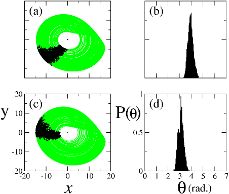
Figure 1: PS at $\epsilon=0.04$ in coupled Rössler oscillators: $\dot{x}_{1}=-\omega_{d}y_{1}-z_{1}$, $\dot{y}_{1}=\omega_{d}x_{1}+0.15y_{1}$, $\dot{z}_{1}=0.2+z_{1}(x_{1}-10)$, $\dot{x}_{2,3}=-\omega_{r}y_{2,3}-z_{2,3}$, $\dot{y}_{2,3}=\omega_{r}x_{2,3}+0.165y_{2,3}+\epsilon(y_{1}-y_{2,3})$, $\dot{z}_{2,3}=0.2+z_{2,3}(x_{2,3}-10)$, where $\omega_{d}=1.015$ and $\omega_{r}=1.0$. (a) stroboscopic phase trajectory (black dots) of oscillator 1 with reference oscillator 3 Strobo . Gray dots show the whole attractor of oscillator 1 without stroboscopic sampling. (c) stroboscopic phase trajectory (black dots) of oscillator 2 with reference oscillator 3. (b) and (d) probability distributions of (a) and (c), respectively.

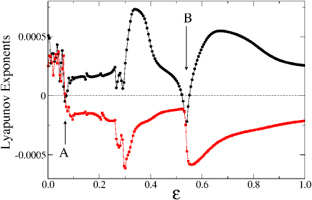
Figure 2: Two largest transverse Lyapunov exponents when $\omega_{d}=0.7$ and $\omega_{r}=1.0$. There are two transition points, A and B.

Next, we consider two response Rössler oscillators driven by the correlated signals, $x_{1}$ and $y_{1}$, instead of identical ones:

$$\dot{x}_{1} = -\omega_{d}y_{1}-z_{1},$$

$$\dot{y}_{1} = \omega_{d}x_{1}+0.165y_{1},$$

$$\dot{z}_{1} = 0.2+z_{1}(x_{1}-10),$$ (2)

$$\dot{x}_{2} = -\omega_{r}y_{2}-z_{2}+\epsilon(x_{1}-x_{2}),$$

$$\dot{y}_{2} = \omega_{r}x_{2}+0.165y_{2},$$

$$\dot{z}_{2} = 0.2+z_{2}(x_{2}-10),$$ (3)

$$\dot{x}_{3} = -\omega_{r}y_{3}-z_{3},$$

$$\dot{y}_{3} = \omega_{r}x_{3}+0.165y_{3}+\epsilon(y_{1}-y_{3}),$$

$$\dot{z}_{3} = 0.2+z_{3}(x_{3}-10),$$ (4)

where the correlated signal $x_{1}$ and $y_{1}$ of oscillator 1 are fed into oscillators 2 and 3, respectively. In real systems, noise and delay in propagating channel are unavoidable. Thus the above system models a real situation in which two response systems are driven by correlated signals, $x$ and $x^{\prime}$ where $x^{\prime}$ is a distorted version of $x$. We propose the above system for studying PS in unidirectionally coupled systems and its relation to GS.

The difference dynamics between two response oscillators is given by $\Delta\dot{\bf X}=A\Delta\bf{X}+{\Xi}(t)$ where $\Delta{\bf X}={\bf x_{2}}-{\bf x_{3}}$, $A=((0,-\omega_{r},-1),~{}(\omega_{r},0.165,0),~{}(0,0,-10))$, and ${\bf\Xi}=\mbox{diag}(\epsilon(x_{1}-x_{2}),~{}-\epsilon(y_{1}-y_{3}),~{}z_{2}x_{2}-z_{3}x_{3})$. By iterating this dynamics, we can find transverse Lyapunov exponents describing the relative motion of oscillators 2 and 3. In Fig. 2, we see two transition points, A and B, which, as we will see below, correspond to two different types of PS: namely, GPS at A and the conventional PS at B.

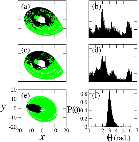
Figure 3: GPS in Eq. (2)-(4) at $\epsilon=0.2$: (a) stroboscopic phase trajectory (black dots) of oscillator 1 with oscillator 3 Strobo ; (c) oscillator 1 with oscillator 2; (e) oscillator 3 with oscillator 2; (b) (d) (f) probability distributions of (a), (c), and (e), respectively.

The phase difference between drive and response oscillators is given by

$$\dot{\phi}_{1k} = \Delta\omega-B(\theta_{1},\theta_{k})\sin\phi_{1k}+\eta_{k}(\theta_{1},\theta_{k}),$$ (5)

where, $\Delta\omega=\omega_{d}-\omega_{r}$,

$$B(\theta_{1},\theta_{k}) = \frac{\epsilon}{2}\frac{R_{1}}{R_{k}}-0.15\cos(\theta_{1}+\theta_{k}),$$

$$\eta_{k}(\theta_{1},\theta_{k}) = \frac{\epsilon(2k-5)}{2}\frac{R_{1}}{R_{k}}\sin(\theta_{1}+\theta_{k})$$

$$-(0.015-\epsilon)\sin\theta_{k}\cos\theta_{k}$$

$$+(\frac{z_{1}}{R_{1}}\sin\theta_{1}-\frac{z_{k}}{R_{k}}\sin\theta_{k}).$$

We can see a $k$-dependent term in $\eta_{k}(\theta_{1},\theta_{k})$ which is due to the driving by correlated signals from the drive oscillator in Eq. (2)-(4). We can obtain the critical point for PS transition which is $\epsilon_{c}=-2\Delta\omega=0.6$, in accordance with the argument of the former case (below Eq. (1)). The drive and response oscillators develop to a PS state at this critical value and PS between oscillators 2 and 3 is induced above this critical coupling. The critical value of the critical coupling agrees with that of the transition point indicated by point B ($\epsilon\approx 0.55$). Thus we understand that B corresponds to conventional PS transition point at which the three oscillators develop to PS simultaneously.

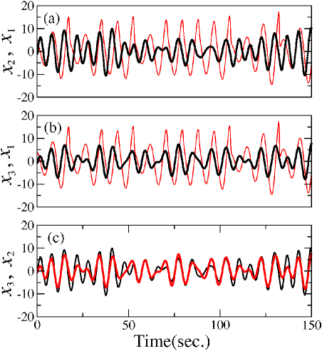
Figure 4: Temporal behaviors of drive and response oscillators in the GPS regime when $\epsilon=0.2$: (a) $x_{1}$ and $x_{2}$ (b) $x_{1}$ and $x_{3}$ (c) $x_{2}$ and $x_{3}$.

We need to inspect the phenomenon at reference point A, which is described as crossing to the negative value in one of the Lyapunov exponents. Fig. 3 shows the trajectories in phase space and probability distributions near reference point A. A PS state appears only in the response-response system (Fig. 3 (e) and (f)) without PS in the drive-response system (because probability distributions are not localized in Fig. 3 (a)-(d)), which is different from the case of the reference point B. We call this phenomenon GPS on the analogy of GS in which two state variables, ${\bf x}_{2}$ and ${\bf x}_{3}$ coverge to the same value. In GPS the phases $\theta_{2}$ and $\theta_{3}$ are bounded by a constant. Figure 4 shows the temporal behaviors of each oscillator at the same coupling strength as that of Fig. 3. We note that PS is established in oscillator 2 and 3 as the phases are mostly matched in Fig. 4 (c), while phase slippings appear in oscillators 1 and 2 (Fig. 4 (a)) or oscillators 1 and 3 (Fig. 4 (b)), intermittently. Finally, we remark that GPS is a novel phenomenon characterized by PS in the response-response system, and thus it is different from conventional PSPhaseSync .

In Fig. 5, we also observe that GPS appears when the responses are slightly detuned with frequencies of $1.0\pm 0.005$, and it destabilizes for frequencies of $1.0\pm 0.01$. This implies that GPS is a real phenomenon that should be experimentally observable Remark . And the attractor deformations observed in Fig. 3 (e) and Fig. 5 (e) seem to be originated from the driving signal of different natural frequency. The similar phenomenon is often observed in unidirectionally coupled systems with different dynamics GenSync . It was shown recently PhaseSync ; Lee that the phase defined by geometrical function like ours and the phase based on the Hilbert transformation practically coincide. So we think our result is independent of the method of defining the phase.

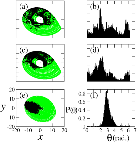
Figure 5: Appearance of GPS when two response oscillators are slightly detuned. The natural frequencies of response oscillators are $w_{r}=1.005$ (of oscillator 2) and $w_{r}=0.995$ (of oscillator 3), respectively. Others parameters are those of Fig. 3.

In conclusion, we have studied PS in unidirectionally coupled chaotic systems with parameter mismatch. And we have focusedly clarified the relationship of PS phenomena in the drive-response and PS in the response-response systems. When the driving signals are identical, PS in the drive-response system corresponds to PS in the response-response system and the system develops to GS as the coupling strength increases: PS$\rightarrow$GS. When the driving signals are correlated (but not identical), PS is established in the response-response system but not the drive-response system. We call this phenomenon GPS. The GPS state transits to PS when coupling strenght increases. The results are confirmed by the analysis of Lyapunov exponents, phase trajectories, and time series. We expect that the GPS concept could be used for analyzing weak interdependences of data coming from weakly correlated systems such as neuronal systems NeuronSync , cardiac oscillators Card , and ecological systems eco etc.

The authors thank J. Kurths, S.-Y. Lee, and M.S. Kurdoglyan for helpful discussions. This work is supported by Creative Research Initiatives of the Korean Ministry of Science and Technology.

References

- (1) Ch. Huygens, Horologium Oscillatiorium. Apud F. Muguet, Parisiis, France, 1673. English translation: The Pendulum Clock, Iowa State University Press, Ames, 1986.
- (2) H. Fujisaka and T. Yamada, Prog. Theor. Phys. 69, 32 (1983); V.S. Afraimovich, N.N. Verichev, and M.I. Rabinovich, Radiophys. Quantum Electron. 29, 747 (1986).
- (3) L.M. Pecora and T.L. Carroll, Phys. Rev. Lett. 64, 821 (1990)
- (4) D.J. DeShazer, R. Breban, E. Ott, and R. Roy, Phys. Rev. Lett. 87, 044101(2001); K.V. Volodchenko, V.N. Ivanov, and S.-H. Gong et al., Optics Letters 26, 1406 (2001).
- (5) C.M. Kim, G.S. Yim, J.W. Ryu, and Y.J. Park, Phys. Rev. Lett. 80; L. Zhu and Y.-C. Lai, Phys. Rev. E 64, 045205 (2001).
- (6) R.C. Elson, A.I. Selverston, and R. Huerta et al., Phys. Rev. Lett. 81, 5692 (1998).
- (7) L. Kocarev and U. Parlitz, Phys. Rev. Lett. 74, 5028 (1995) and references therein.
- (8) D.J. DeShazer, R. Breban, E. Ott, and R. Roy, Phys. Rev. Lett. 87, 044101 (2001).
- (9) M. Rosenblum, A. Pikovsky, and J. Kurths, Phys. Rev. Lett. 76, 1804 (1996).
- (10) K.J. Lee, Y. Kwak, and T.K. Lim, Phys. Rev. Lett. 81, 321 (1998); E. Rosa, E. Ott, and M.H. Hess, Phys. Rev. Lett. 80, 1642 (1998); K. Josić and D.J. Mar, Phys. Rev. E64, 056234 (2001).
- (11) W.-H. Kye and C.-M. Kim, Phys. Rev. E 62, 6304 (2000).
- (12) M. Rosenblum, A. Pikovsky and J. Kurths, Phys. Rev. Lett. 78, 4193 (1997).
- (13) L. Kocarev and U. Parlitz, Phys. Rev. Lett. 76, 1816 (1996); R. Brown, Phys. Rev. Lett. 81, 4835 (1998); N.F. Rulkov, M.M. Sushchik, L.S. Tsimring, and H.D.I. Abarbanel, Phys. Rev. E51, 980 (1995).
- (14) U. Parlitz, L. Junge, and W. Lauterborn, Phys. Rev. E 54, 2115 (1996).
- (15) Z. Zheng and G. Hu, Phys. Rev. E 62, 7882 (2000).
- (16) R. Q. Quiroga, A. Kraskov, T. Kreuz, and P. Grassberger, Phys. Rev. E65, 041903 (2002).
- (17) T. Yalcinkaya and Y.-C. Lai, Phys. Rev. Lett. 79, 3885 (1997).
- (18) One can collect the values of projective coordinate or phase value of a target oscillator, whenever a reference oscillator crosses a Poincaré section, e.g., we take . In this case we say that the plot of the values of is the stroboscopic trajectory in phase space with the reference oscillator. is the corresponding phase. The probability distribution is the normalized histogram of the stroboscopic phases.
- (19) On the other hand, we could not observe GPS regime in the case .
- (20) C. Schäfer, M.G. Rosenblum, H. Abel, and J. Kurth, Phys. Rev. E60, 857 (1999).
- (21) B. Blasius, A. Huppert, and L. Stone, Nature 399, 354 (1999).