A Cross-Over in the Enstrophy Decay in Two -Dimensional Turbulence in a Finite Box

Abstract

The numerical simulation of two-dimensional decaying turbulence in a large but finite box presented in this paper uncovered two physically different regimes of enstrophy decay. During the initial stage, the enstrophy $\Omega$, generated by a random Gaussian initial condition, decays as $\Omega(t)\propto t^{-\gamma}$ with $\gamma\approx 0.7-0.8$. After that, the flow undergoes a transition to a gas or fluid composed of distinct vortices. Simultaneously, the magnitude of the decay exponent crosses over to $\gamma\approx 0.4$. An exact relation for the total number of vortices, $N(t)$, in terms of the mean circulation $\Gamma$ of an individual vortex $N(t)\propto 1/\overline{\Gamma^{2}}$ is derived. A theory predicting $N(t)\propto t^{-\xi}$ and the magnitudes of exponents $\gamma=2/5$ and $\xi=4/5$ is presented and the possibility of an additional very late-time cross-over to $\gamma=1/3$ and $\xi=2/3$ is also discussed.

The interest in the problem of two-dimensional (2D) turbulence was excited by the pioneering work of Onzager¹, who recognized the role of point-vortices in 2D turbulence dynamics and suggested a theory based on some general concepts of statistical physics. In Onzager’s days the quantitative investigation of two-dimensional hydrodynamics was inhibited by the pausity of well-controlled physical experiments. Now, with advent of powerful computers, various features of the problem are much better understood due to the remarkable works of McWilliams and collaborators^2-5, Benzi et. al.⁶ and many others. Still, many important questions remained unanswered.

If a fluid in a large three-dimensional vessel of linear dimension $L$ is stirred on a length-scale ${\cal L}\ll L$, the non-linear process of generation of the small-scale velocity fluctuations leads to energy dissipation, making a steady state possible even in the limit of vanishing viscosity. In this case, universality means independence of the small-scale features of the flow upon length-scale $L$. In two dimensions, the situation is very different; the Euler equations conserve both energy and enstrophy. As a result, the most prominent dynamic feature of 2D-turbulence are two fluxes in the wave-number space⁷. The (negative) energy flux leads to formation of the slow-varying (low-frequency) large-scale motions containing almost the entire energy of the system on a time-dependent integral scale $l_{0}(t)$. The second, enstrophy flux, leads to generation of rapidly-varying small-scale velocity fluctuations responsible for the enstrophy of the flow. The short-time dynamics, when $l_{0}(t)/L\ll 1$, are characterized by a quasi-steady inertial range with the energy spectrum $E(k)\propto k^{-\frac{5}{3}}$ and the integral scale $l_{0}(t)\approx 2\pi/k_{0}(t)\propto t^{\frac{3}{2}}\ll L$. The most interesting phenomenon happens later in the evolution when $l_{0}(t)\approx L$; the energy spectrum starts piling up at $k\approx\pi/L$ forming very slow varying and very powerful motions where the major fraction of kinetic energy is concentrated^8-13. The enstrophy associated with these motions is negligibly small. Simultaneously, powerful small-scale vortices, containing almost the entire enstrophy of the flow, are formed at the centers of these large scale structures. The characteristic scale (radius),$a(t)\approx 1/k_{f}\approx const$, of these vortices is very small, $a(t)\ll L$. These complex structures depend on geometry of the problem and thus are not universal^8,12.

The time evolution of decaying two-dimensional turbulence also has three distinct intervals. During the initial stage, the ”inverse cascade” leads to population of the scales $k<k_{0}(t=0)$ with formation of vortices which merge and create the ever larger vortices. At the same time the enstrophy dissipation and some intermittency are generated around small-scales¹⁴. The total kinetic energy in the system remains almost constant while the vortex merger persists until only two coherent vortices with positive and negative vorticity are formed (McWilliams²).

Depending on the setup, the experimental and numerical data on the enstrophy decay vary rather dramatically. It has been shown that after some transient, the enstrophy $\Omega$, in turbulence initially generated as a Gaussian random velocity field, decays with time as $\Omega(t)\approx t^{-\gamma}$ with $\gamma\approx 0.7-0.8^{15}$. The recent theory¹⁶ of 2D-turbulence decay in an infinite system led to an asymptotic magnitude $\gamma=2/3$, which is close to numerical results. Later in the evolution, after a substantial depletion of the initial enstrophy, formation of the well-separated vortices containing almost entire enstrophy of a flow has been observed². This phenomenon inspired various investigators to study the dynamics of 2D-turbulence as evolution of a set of initially created point-vortices^3-6. This set up, however, yielded a different decay law for $\Omega(t)$ with $\gamma\approx 0.35-0.4^{2-6}$.

To explain this magnitude of the decay exponent, Carnevale et.al.³ based their scaling theory on numerical results by McWilliams² giving the total number of vortices in a flow $N\approx t^{-\xi}$ with $\xi\approx 0.7-0.75$. More recent simulations by Bracco et al⁴ confirmed this result giving $\xi=0.75\pm 0.05$. Observing that the entire kinetic energy, $K$, of the system is concentrated in a rotational motion of the well-separated vortices, the authors of Ref.[3] obtained $K\approx\rho N(t)\omega^{2}_{o}a^{4}=const$ and assuming that the peak vorticity of a vortex $\omega_{o}\approx const$, they obtained their decay law: $a(t)\propto N^{-\frac{1}{4}}$ $\Omega(t)\approx N(t)\omega_{o}^{2}a^{2}(t)\propto t^{-\frac{\xi}{2}}$ in a good agreement with numerical data. The observed value of the exponent $\xi\approx 0.75$ remained unexplained. The theory of Benzi et. al.⁶ was based on similar assumptions and led to almost qualitatively identical results. Unification of the outcomes obtained from these different setups is one of the goals of the work described below.

In this paper we report the results of a numerical investigation of the 2D turbulence decay in a large but finite square. (The definition of ”large” is given below.) It is shown that after an initial enstrophy decay, characterized by $\gamma\approx 0.7-0.8$, the flow undergoes transition to a state that can be represented as a gas of vortices. The enstrophy decay law in this state is $\Omega\propto t^{-\gamma}$ with $\gamma\approx 0.4$. The theory developed in this paper leads to the characteristic length-scale of a vortex $a(t)\propto N^{-\frac{1}{4}}$ exactly as in Ref.[3]. The proposed analytic model for the vortex interaction gives for the number of vortices in a system as $N(t)\propto t^{-0.8}$ and $\Omega\propto t^{-\frac{2}{5}}$, and are in a close agreement with numerical simulations. An exact expression for $N(t)\propto 1/\overline{\Gamma^{2}}$, where $\Gamma$ is a circulation of an individual vortex, is derived directly from the Navier-Stokes equations.

The problem of decay of two-dimensional (2D) turbulence we are interested in this paper is formulated in a following way. Consider a time evolution of an initial velocity field, $u(x,y,0)={\bf u}_{0}$. defined on a two-dimensional square such that $-L\leq x,y\leq L$. The field $u_{0}$ is a Gaussian random noise defined in the Fourier space in the vicinity of $k=k_{0}(t=0)=O(\frac{N\pi}{L})$ with $\overline{{\bf u}^{2}_{0}}=O(1)$ and $N=const=O(1)$. At the initial instant, $t=0$, the enstrophy is $\Omega=\overline{\omega^{2}}=\overline{(\nabla\times{\bf u})^{2}}=O(1)$. The square is large meaning that we are interested in the limit $\nu\rightarrow 0$ and $k_{0}(t=0)L\rightarrow\infty$. Still, the box is finite so we will be able to study both short time, when $k_{0}(t)L\gg 1$, and long time asymptotics when $k_{0}(t)L\approx 1$. In all our simulations the initial kinetic energy of the flow $K(t=0)=\frac{1}{2}\rho\int v^{2}({\bf x},t=0)d{\bf x}=\frac{1}{2}$ and the fluid density $\rho=1$.

The Navier-Stokes equations with the $O(\nu_{4}\nabla^{4}{\bf v})$ hyper-viscous dissipation terms were simulated using a pseudo-spectral method. To be sure that hyper-viscosity did not influence the results, two simulations with resolutions $1024^{2}$ and $2048^{2}$ were conducted. The initial random field was Gaussian with energy spectrum $E(k)=a_{s}\frac{K}{\rho k_{p}}\left(\frac{k}{k_{p}}\right)^{2s+1}e^{-\left(s+\frac{1}{2}\right)\left(\frac{k}{k_{p}}\right)^{2}}$ where $a_{s}=\frac{(2s+1)^{(s+1)}}{2^{s}s!}$ and $s=3$ as in Ref.[15]. The parameters of the simulations are given in the following table.

N	time-step	$\frac{2K}{\rho}$	$\Omega(t=0)$	$k_{p}$	$\nu_{4}$
$1024$	$0.0005$	$1$	$1170$	$32$	$2.1x10^{-10}$
$2048$	$0.00025$	$1$	$1170$	$32$	$9.6x10^{-11}$

Table 1: Numerical simulation parameters

On Fig.1 we show the time evolution of both enstrophy, $\Omega$, and energy, $K$, in a flow. During the entire simulation, kinetic energy stays constant; this is not so for the enstrophy. Initially after some transient, the enstrophy $\Omega(t)$ obeys the power law $\Omega\propto t^{-\gamma}$ with $\gamma\approx 0.7-0.8$ and is very close to the result reported before by Chasnov¹⁵. Later in the evolution, when the dimensionless time $T$ is such that $T=\sqrt{\overline{\omega^{2}}(t=0)}t\geq 200$, a cross-over to the value $\gamma\approx 0.4$ is clearly seen. On Figs. 2-3 the time evolution of vorticity field is presented. We can observe that the cross-over to a new long-time decay regime ($T\geq 200$), with $\gamma\approx 0.4$, is accompanied by formation of the well-separated distinct vortices. It is interesting, that similar structures were observed in case of the small-scale forced 2D-turbulence^9,10. One feature of Figs. 2-3 deserves a special attention. At the initial stage of decay, $10\leq T\leq 200$, the vortices are more or less homogeneously packed, while at the later times the vortex density shows a clear tendency of the flow structures to clamp together keeping the mean distance between the neighbors more or less constant. This may be an indication of a weakening of the screening of the inter-vortex interaction as the vortex density decreases. The merger itself happens in two stages; first the same-sign vortices approach each other with translational velocity $v_{o}$ and start moving as a couple (”vortex molecule”) rotating around their mutual center of mass. The merging process is relatively slow meaning that during this ”pre-merger” period, the characteristic frequency of this joint motion is $\omega_{m}$ where $\omega_{m}\approx v_{o}/a(t)\ll\omega_{o}$ and $\omega_{o}$ is the mean angular velocity of an individual vortex. This ”dance” is interrupted by a collapse with a single emerging vortex with the peak vorticity $\omega_{o}\approx constant$.

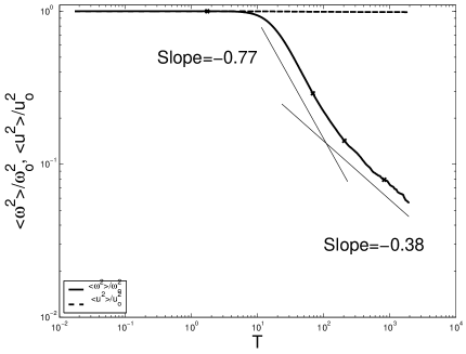
(a) ($1024^{2}$)

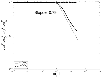
(b) ($2048^{2}$)

Figure 1: Enstrophy and energy decay as function of time

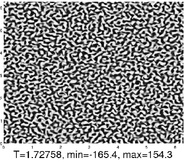
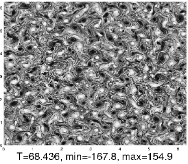
Figure 2: Vorticity field before crossover ($1024^{2}$)

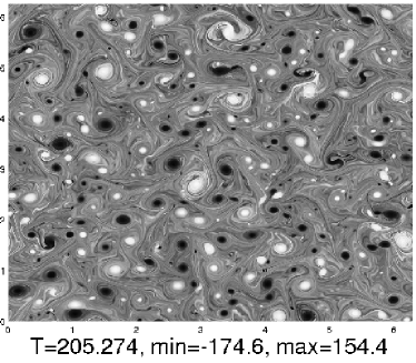
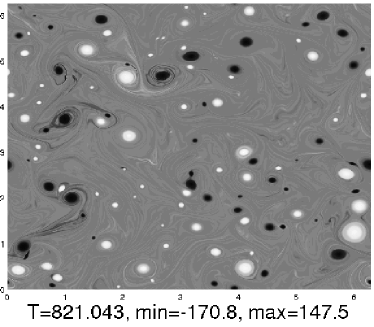
Figure 3: Vorticity field during and after crossover ($1024^{2}$)

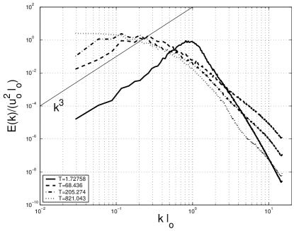
Figure 4: Time evolution of energy spectrum ($1024^{2}$)

First we present a model which is a generalization of a remarkable work by Carnevale et.all.³. After that we will demonstrate its consistency with the Navier-Stokes equations. The total kinetic energy of a flow ($[K]=grcm^{2}/sec^{2}$) is:

$$K(t)=\frac{\rho}{2}\int v^{2}({\bf x})d^{2}x=\frac{1}{2}\rho N(t)[v_{o}^{2}a^{2}+\omega_{o}^{2}a^{4}]=K(t=0)=O(1)=constant$$ (1)

We conjecture and later verify that while the $O(v_{o}^{2}a^{2})$ contribution to the total energy is small, it entirely dominates the time-scale of the merger process. According to Carnevale et al³ and our own numerical simulations we assume that $\omega_{o}\approx const$. Neglecting the $O(v_{o}^{2})$ , the equation (1) leads to the estimate obtained in Ref.[3]: $\frac{1}{2}\rho N(t)\omega_{o}^{2}(t)a(t)^{4}=K=const$ and $a(t)\approx(\frac{2K}{\rho N(t)\omega_{o}^{2}})^{\frac{1}{4}}\propto N^{-\frac{1}{4}}$

Following Carnevale et al³, we introduce the mean distance between the nearest- neighbor vortices as $R\approx L/\sqrt{N(t)}$ and estimate translational velocity $v_{o}$ of a vortex moving in the field of other vortices: as:

$$v_{o}\approx\frac{\Gamma}{R(t)}\approx\frac{\omega_{o}a^{2}\sqrt{N}}{L}=\sqrt{\frac{2K}{L^{2}\rho}}\equiv V$$ (2)

where $\Gamma\approx\omega_{o}a^{2}$ is a circulation. To complete the argument, we estimate the rotational velocity of a vortex as: $v_{R}\approx\omega_{o}a(t)=(\frac{2K\omega_{o}^{2}}{\rho N(t)})^{\frac{1}{4}}$. Thus, the ratio $\frac{v_{o}}{v_{R}}=(\frac{V^{2}}{\omega_{o}^{2}L^{2}})^{\frac{1}{4}}N^{\frac{1}{4}}\propto t^{-\frac{\xi}{4}}\rightarrow 0$ and is indeed small. It is important that according to the above estimate, while $v_{R}$ grows with time, translational velocity $v_{o}$ is a time-independent constant.

Now we need a model for $N(t)$. We consider a vortex merger process as a binary “chemical reaction” $2N\Longrightarrow N$ with the ”reaction rate” ${\cal R}(t)$, where is the inverse of the time the vortex pair spends in a bound state prior to the merger event. If vortices are well separated, the population equation is:

$$\frac{dN}{dt}=-{\cal R}N^{2}(t)$$ (3)

We recall that two same-sign vortices attract each other, tending to form a spinning dipole (bound state) with the linear dimensions (radius of the orbit) depending upon the impact parameter, relative translational velocity, and other characteristics of the collision process. It is important that the larger the relative velocity , the larger the radius of an orbit of a bound state. The rotational frequency of this bound pair is $O(v_{o}/I)$ where $I$ is the impact parameter. In the system we are dealing with, the binary collisions happen in the field of other vortices of both signs often strongly perturbing the pre-merging dipole. It is clear, and we observe it in our simulations, that only the most strongly interacting pairs stay stable under perturbations from surrounding fluid long enough to eventually merge. The most stable ones are those with linear dimension (impact parameter) not larger than a few $a(t)$ and having smallest relative velocity. Since the translational velocity $v_{o}\approx const$, describing the motion of coupled vortex pair before the merger event, is the smallest velocity-scale in the system we choose it as a rate determining parameter. The merger rate is thus estimated as: ${\cal R}\approx v_{o}/a(t)\approx v_{o}(\frac{N(t)\omega_{o}^{2}\rho}{2K})^{\frac{1}{4}}=\frac{v_{o}}{L}\sqrt{\frac{\omega_{o}L}{v_{o}}}N^{\frac{1}{4}}$. Substituting this into the above differential equation gives:

$$N=\frac{N_{0}}{(\frac{t}{t_{0}}+1)^{\frac{4}{5}}}\rightarrow N_{0}(\frac{t}{t_{0}})^{-\frac{4}{5}}$$ (4)

where $t_{0}\approx\sqrt{\frac{L}{v_{o}\omega_{o}}}$ and $N_{0}$ is an undetermined constant. This gives the enstrophy decay law as $\Omega(t)\approx N(t)\omega_{o}^{2}a^{2}(t)\propto t^{-\frac{2}{5}}$ and is extremely close to numerical result. It follows from (4) that in an infinite system ($L\rightarrow\infty$) the cross-over to $\gamma\approx 0.4$ never happens and the enstrophy decay process with $\gamma=2/3$ persists in the limit $t\rightarrow\infty$. Now we would like to discuss another possibility. If the mean distance between the nearest vortices is large ($R=O(L/\sqrt{N(t)}$), then the reaction rate ${\cal R}=O(v_{o}\sqrt{N}/L)$ and equation (5) gives $N(t)\propto t^{-\frac{2}{3}}$ and $\Omega(t)\propto t^{-\frac{1}{3}}$.

The relations derived above are the outcome of a kinetic-like considerations. It is interesting to verify their consistency with the Navier-Stokes equations. Choosing the displacement vector ${\bf r}$ parallel to the $x$-axis and assuming statistical homogeneity and isotropy of a flow , the Navier-Stokes equations lead to the relation for the correlation function of the scalar vorticity $D_{\omega}=\overline{\omega(x)\omega(x+r)}^{16-19}$:

$$\frac{\partial D_{\omega}}{\partial t}=-\frac{1}{4r}\frac{\partial}{\partial r}r\overline{(v(x+r)-v(x))(\omega(x+r)-\omega(x))^{2}}$$ (5)

Multiplying this equation by $r$ and integrating over the interval $0\leq r\leq L$ gives^16-18:

$$\frac{\partial}{\partial t}\int drr\overline{\omega(x+r)\omega(x)}=-\frac{1}{4}r\overline{(v(x+r)-v(x))(\omega(x+r)-\omega(x))^{2}}|^{L}_{0}$$ (6)

In the limit $L\rightarrow\infty$ the right side of this equation is equal to zero. To evaluate the integral, we recall that in 2D hydrodynamics the point-vortex representation of vorticity is: $\omega({\bf x})=\sum_{i}\Gamma_{i}\delta({\bf x}-{\bf X}_{i}(t))$, where ${\bf X}_{i}(t)$ is a position of the $i^{th}$ vortex and $\Gamma_{i}$ stands for its circulation. Then, recalling that the flow is filled with vortices of both signs so that $\sum_{i\neq j}\Gamma_{i}\Gamma_{j}=0$, we derive readily:

$$\int dr~{}r\overline{\omega({\bf x})\omega({\bf x}+r{\bf i})}=\int d{\bf r}\frac{1}{2\pi L^{2}}\sum_{i,j}\Gamma_{i}\Gamma_{j}\int d{\bf x}\delta({\bf x-X_{i}(t)})\delta({\bf x-X_{j}(t)}+r{\bf i})=$$

$$\sum_{i,j}\frac{\Gamma_{i}\Gamma_{j}}{2\pi L^{2}}=\sum_{i=1}^{N(t)}\frac{\Gamma_{i}^{2}}{2\pi L^{2}}=\frac{N(t)\overline{\Gamma^{2}}}{2\pi L^{2}}\approx\frac{N(t)\omega_{o}^{2}a^{4}}{2\pi L^{2}}\approx const~{}~{}~{}~{}~{}~{}~{}~{}~{}~{}~{}~{}~{}~{}~{}~{}~{}~{}~{}~{}~{}~{}~{}~{}~{}~{}~{}~{}~{}~{}~{}~{}~{}~{}~{}~{}~{}~{}~{}(7)$$

This relation, derived from purely hydrodynamic considerations, is quite important since it serves as a correct definition of both $\omega_{o}$ and $a(t)$ which are the basic ingredients of the ”kinetic theory” developed in Carnevale et.al³. The average- splitting $\overline{\Gamma^{2}}\approx\omega_{o}^{2}a^{4}$, used in derivation of the last relation in (7) is an approximation valid only if the peak vorticity and vortex radius are statistically independent. At the present time we cannot assess the quality of this approximation.

We can also start with the Navier-Stokes equations and write equation for the correlation function of the $x$-component of velocity field ( here denoted as $v$)^16-18:

$$\frac{\partial}{\partial t}\overline{v(x+r)v(x)}=\frac{1}{6r^{3}}\frac{\partial}{\partial r}r\overline{(v(x+r)-v(x))^{3}}$$

Repeating the considerations leading to (6) we obtain: $\int r^{3}\overline{v({\bf x})v({\bf x}+{\bf i}r)}dr=const$ and introducing the correlation length $a(t)$, this integral is estimated readily giving $N(t)v^{2}a^{2}\approx N(t)(v_{o}^{2}+\omega_{o}^{2}a^{4})\approx const$ where $N(t)=L^{2}/a^{2}$. This is exactly the relation (1) evaluated above from the energy conservation considerations.

The main result of this work is unification of the two different exponents $\gamma\approx 0.7-0.8$ and $\gamma\approx 0.4$ as corresponding to intermediate and long time regimes of the enstrophy decay in 2D turbulence, respectively. The exact relation $N(t)\propto 1/\overline{\Gamma^{2}}$ derived from the Navier-Stokes equation, is a direct generalization of an approximate formula $N(t)\propto a^{-4}$ obtained by Carenevale et.al.³ using the ”kinetic theory” approach and assuming the constancy of the peak vorticity of individual vortices.

We have identified three possible values of exponent $\gamma$. According to ref.[16], the initial stage of enstrophy decay in a large box ($\L\rightarrow\infty$) is characterized by $\gamma=2/3$ which is close to results of numerical simulations by Chasnov¹⁵ and the ones presented in this paper. It has been demonstrated that in a finite box, after the depletion of the initial externally introduced enstrophy, a flow composed of long-living distinct vortices emerges and the exponent crosses over to $\gamma\approx 0.4$, very close our theoretical prediction. Another cross-over to $\gamma\approx 1/3$ and $\xi=2/3$ as a very long-time asymptotics in a system with small number of vortices is predicted. To the best of our knowledge, this regime has not yet been observed.

The nature of the transition remains poorly understood. It has been shown^9-10 that in case of the small-scale forced 2D turbulence, the well-separated vortices emerge as a result of the finite-size effect (condensation). It is hard to say if this conclusion holds for freely decaying 2D turbulence but if it does, then the question of universality of exponents $\gamma$ and $\xi$ becomes extremely interesting and important. Some indications that the finite-size effects can play an important role can be found from Figs.1-4. It can be shown theoretically that as long as $k_{0}(t)L\gg 1$, the large-scale energy spectrum in this developing flow is $E(k\ll k_{0}(t))\propto k^{3}\phi(t)$. We can see that in the short-time interval, $T<200$, this is indeed approximately correct and the exponent is $\gamma\approx 0.7-0.8$. At the longer times ($T>200$), when $k_{0}(t)L\approx 1$, the energy spectrum starts strongly deviate from the $k^{3}$-curve. This is definitely due to the finite size- effects. Simultaneously, the well-separated vortices emerge and the exponent crosses over to $\gamma\approx 0.4$.

References.

1. L. Onzager, Nuovo Cimento 6(2), 279 (1949)
2 . J.C. McWilliams, J.Fluid Mech 219, 361 (1990)
3. G.F.Carnevale, J.C.McWilliams, Y.Pomeau, J.B.Weiss and W.R.Young, Phys.Rev.Lett.66, 2735 (1991).
4.A.Bracco, J.C.McWilliams, G.Murante,A.Provenzale,J.B.Weiss, Phys.Fluids 12, 2931 (2000).
5. M.V.Melander, J.C.McWilliams, and N.Zabusski, J.Fluid mech. 178, 137 (1987).
6 R.Benzi, S.Patarnello and P.Santangelo, J.Phys.A 21, 1221 (1988)
7. R.H.Kraichnan, Phys.Fluids 10, 1417 (1967)
8. U. Frisch and P-L Sulem, Phy.Fluids 27, 1921 (1984)
9. L.M. Smith and V.Yakhot, Phys.Rev.Lett. 71, 352 (1993)
10. L.M. Smith and V. Yakhot, J.Fluid Mech. 274 (1994)
11. G.Bofetta, A.Celani and M. Vergassola, Phys. rev.E 61, R29 (2000).
12. J. Paret and P. Tabeling, Phys. Fluids 12, 3126 (1998)
13. R.H.Kraichnan and D. Montgomery, Reports Prog.Phys. 43, 547 (1980)
14. L.M. Smith V. Yakhot, Phys.Rev.E55, 5458 (1997)
15. J.R.Chasnov, Phys. Fluids 9, 171 (1997)
16. V.Yakhot, Phys.Rev.Lett. 2004 (in press).
17. A.S. Monin and A.M.Yaglom, vII, The MIT press, Cambridge, 1975
18. L.D. Landau and E. M. Lifshitz, Pergamon Press, Oxford, 1982
19. L.G. Loitsyanskii,Trudy Tsentr. Aero.-Gidrodyn. Inst., 3, 33 (1939), (in Russian)