Optical pulse propagation in fibers with random dispersion

Abstract

The propagation of optical pulses in two types of fibers with randomly varying dispersion is investigated. The first type refers to a uniform fiber dispersion superimposed by random modulations with a zero mean. The second type is the dispersion-managed fiber line with fluctuating parameters of the dispersion map. Application of the mean field method leads to the nonlinear Schrödinger equation (NLSE) with a dissipation term, expressed by a 4th order derivative of the wave envelope. The prediction of the mean field approach regarding the decay rate of a soliton is compared with that of the perturbation theory based on the Inverse Scattering Transform (IST). A good agreement between these two approaches is found. Possible ways of compensation of the radiative decay of solitons using the linear and nonlinear amplification are explored. Corresponding mean field equation coincides with the complex Swift-Hohenberg equation. The condition for the autosolitonic regime in propagation of optical pulses along a fiber line with fluctuating dispersion is derived and the existence of autosoliton (dissipative soliton ) is confirmed by direct numerical simulation of the stochastic NLSE. The dynamics of solitons in optical communication systems with random dispersion-management is further studied applying the variational principle to the mean field NLSE, which results in a system of ODE’s for soliton parameters. Extensive numerical simulations of the stochastic NLSE, mean field equation and corresponding set of ODE’s are performed to verify the predictions of the developed theory.

,

1 Introduction

Propagation of optical pulses in fibers with non-uniform dispersion remains to be a field of intensive research. The relevant studies are motivated by their application to modern optical communication systems. Random fluctuations of the dispersion coefficient is inherent to existing optical fibers, which deteriorates the performance of communication lines based on both standard and dispersion-managed solitons [1]. Therefore, the proper compensation of the pulse distortion caused by random fluctuations of the fiber dispersion is of vital importance, especially for long haul optical communication systems.

The previous investigations were concerned with the analysis of the modulational instability (MI) of electromagnetic waves in fibers with random dispersion. It was shown that the randomness can reduce the MI gain for anomalous dispersion region and generate the instability for the whole spectrum of modulations in the normal dispersion region [2, 3, 4]. Recently the performance of dispersion-managed soliton system with random variations of span length and span path-average dispersions has been studied numerically in Ref. [5]. The comprehensive analysis of the dynamics of solitons implies the solution of the nonlinear Schrödinger equation (NLSE) with randomly varying coefficients, which is a rather complex problem. However, in the particular case, when a uniform fiber dispersion is superimposed by weak random modulations, the perturbation theory based on the Inverse Scattering Transform (IST) can be applied. In the framework of this approach the decay law for optical solitons was derived which describes their radiative damping due to emission of linear waves [6, 9]. The case of dispersion-managed (DM) solitons is more complicated because here one has the superposition of the random fluctuations and strong periodic modulations of the dispersion. In recent works [10, 11, 12, 13] the variational approach was employed to analyze the dynamics of optical pulses in systems with random dispersion-management. It was shown that the DM soliton is subject to disintegration due to random variations of the dispersion map parameters. The averaged equation in the frequency domain was derived in [14, 15, 16], where an interesting idea of pinning (compensation of the accumulated effect of fluctuations) is proposed. Numerical simulations of the dynamics of DM solitons in systems with random dispersion-management are presented in [10, 11, 19, 20]. Analytical description of the DM soliton dynamics in fluctuating media remains to be an open problem, since the radiative effects cannot be taken into account in the frame of the variational approach. However, there exists a limit pertaining to strong dispersion-management, where the NLSE with periodic coefficients is nearly integrable [21]. The development of the stochastic perturbation theory similar to the IST approach may be successful in this limit. This problem deserves a separate consideration.

In this study we apply the mean field method (MFM) for the analysis of propagation of optical pulses in fibers with random dispersion, including the DM case. The advantage of this method consists in that, it doesn’t depend on the fact whether the basic deterministic equation is integrable or not.

The paper is organized as follows. In section II we derive the mean field equation for the case of uniform dispersion perturbed by random modulations and compare the predictions of this approach with the corresponding result of the IST based perturbation theory. The condition for the existence of autosoliton in random media is derived. The section III is devoted to analysis of the DM soliton dynamics in the framework of MFM. We show that the variational approach applied to the mean field equation with a frequency dependent damping leads to a system of ODE’s for DM soliton parameters. And in the last section IV, we briefly summarize the main results of this study.

2 Mean field method and IST approach

The propagation of optical pulses in a fiber with uniform dispersion superimposed by random modulations was considered in the framework of the perturbation theory based on the IST [6]. Assuming the perturbation to be of the form $R=\epsilon(z)u_{tt},$ where $\epsilon(z)$ is a weak random process, the radiative decay of a soliton was calculated. The decay law for the pulse amplitude was derived from the energy conservation and the dynamic balance between the radiative component and localized mode. It was shown that the amplitude of the soliton decays with the propagation distance as $1/z^{1/4}$ for $z<1/\sigma^{2}$, where $\sigma^{2}$ is the noise level. In addition, the decay rate was revealed to be highly dependent on the pulse duration $\sim t_{0}^{-4}$, i.e. the influence of the randomness is superior on short pulses, particularly in the femtosecond range.

The extension of this approach for more general cases (e.g. dispersion-managed solitons) is in general not possible. Therefore, it is of interest to apply another approach which is independent on the fact whether the underlying deterministic equation is integrable or not. One of such possibilities is provided by the mean field method [22]. Despite the well known troubles of this approach for random nonlinear wave equations [23, 24], one can obtain reasonably well description in the case of weak fluctuations, and/or small distances of propagation.

In this section we apply the MFM and the perturbation theory based on the IST to the problem of optical pulse propagation in fibers with random dispersion. By comparing the predictions of these two approaches we reveal the limits of validity of the MFM.

Optical pulse propagation in fibers is well described by the NLSE

$$iu_{z}+\frac{d(z)}{2}u_{tt}+|u|^{2}u=i\delta u+i\mu|u|^{2}u.$$ (1)

Here $\delta,\ \mu$ are the coefficients of linear and nonlinear amplification (damping) respectively. In our model these terms are supposed to compensate the damping originated from the randomness of the fiber dispersion. Below we consider the case, when the dispersion coefficient $d(z)$ is the sum of the constant and random parts, i.e. $d(z)=1+\epsilon(z)$ with

$$<\epsilon>=0,\ <\epsilon(z)\epsilon(z^{\prime})>=B(z-z^{\prime},l_{c})_{l_{c}\rightarrow 0}\rightarrow\sigma^{2}\delta(z-z^{\prime}).$$ (2)

The noise is assumed to be small compared to the constant part of the dispersion.

To derive the equation averaged over fluctuations we apply the mean field method, representing the field as consisting of the mean value and small fluctuating part $u=<u>+\delta u,<\delta u>=0,\delta u\ll<u>$, where $<u>$ is a slowly varying mean field. According to this method we can use the decoupling $<|u|^{2}u>\approx|<u>|^{2}u$. This corresponds to neglecting by fluctuations of the nonlinearity, and the approximation is valid for propagation distances $z<<1/\sigma^{2}$. In typical optical experiments this requirement is satisfied. In general the decoupling procedure is inaccurate since the scattered field $\delta u$ grows with propagation distance and becomes comparable with $<u>$, that violates the assumption $\delta u\ll<u>$. In order to decompose the mean $<\epsilon(z)u_{tt}>$ we use the Furutsu-Novikov formula

$$<\epsilon(z)F(u)>=\int_{0}^{z}B(z-z^{\prime})<\frac{\delta F(u)}{\delta\epsilon(z^{\prime})}>dz^{\prime}.$$ (3)

Of particular interest is the case of white noise fluctuations, when $B(x)=\sigma^{2}\delta(x)$. Also the causality principle will be useful

$$\frac{\delta u(z)}{\delta\epsilon(z^{\prime})}=0,\quad\mbox{ if }\ z^{\prime}<0,\ \ z^{\prime}>z.$$ (4)

Then integrating Eq.(1) over $z^{\prime}$ from $0$ to $z$ and taking variational derivative (with the causality principle in mind) we obtain

$$<\epsilon(z)u_{tt}(z,t)>=\frac{i\sigma^{2}}{4}<u>_{tttt}.$$ (5)

In the result we get the equation for averaged pulse profile with a fourth order dissipative term (for simplicity we dropped averaging symbol in $<u(z,t)>$)

$$iu_{z}+\frac{1}{2}u_{tt}+|u|^{2}u=-i\gamma u_{tttt}+i\delta u+i\mu|u|^{2}u,$$ (6)

where $\gamma=\sigma^{2}/4,\ \sigma$ being the noise strength.

As it is apparent from this equation, the effect of random dispersion on the pulse evolution is described as the pulse propagation in a uniform medium with the frequency depending dissipation. Formally this equation coincides with the complex Swift-Hohenberg equation. Thus we can expect the existence of dissipative solitons in nonlinear media with fluctuating dispersion.

At first we examine the decay rate of a pulse under the action of the 4th order dispersion coefficient in Eq.(6). For the weak noise case this term is small and we can apply the perturbation theory. The single soliton propagation is conveniently described using the equations for the energy $N=\int|u|^{2}dt$ and momentum $P=\mbox{Im}(\int u_{t}^{*}udt)$.

$$\frac{dN}{dz}=2\int_{-\infty}^{\infty}[\delta|u|^{2}+\mu|u|^{4}-\gamma|u_{tt}|^{2}]dt,$$ (7)

$$\frac{dP}{dz}=2\mbox{Im}\int_{-\infty}^{\infty}[\delta u+\mu|u|^{2}u+\gamma u_{tttt}]u_{t}^{*}dt.$$ (8)

We look for the single soliton solution in the form

$$u(z,t)=\eta\mbox{sech}[\eta(t+\Omega z)]e^{-i\Omega t+i(\eta^{2}-\Omega^{2})z/2}.$$ (9)

Substituting Eq.(9) into Eqs. (7),(8) we obtain the system of equations for the soliton amplitude and velocity

$$\frac{d\eta}{dz} = 2\eta[\delta-\gamma(\frac{7}{15}\eta^{4}+2\eta^{2}\Omega^{2}+\Omega^{4})+\frac{2}{3}\mu\eta^{2}],$$ (10)

$$\frac{d\Omega}{dz} = -\frac{8}{3}\gamma\Omega\eta^{2}(\frac{7}{5}\eta^{2}+\Omega^{2}).$$ (11)

Parameters $\delta,\mu$ are absent in the second equation, since the soliton velocity is not affected by such type of perturbations. For $\Omega=0$ one can find the decay law of the soliton due to the 4th order dispersive dissipation, which follows from Eq.(10)

$$\eta(z)=\frac{\eta_{0}}{(1+\frac{14}{15}\sigma^{2}\eta_{0}^{4}z)^{1/4}}\approx\eta_{0}(1-\frac{7}{30}\sigma^{2}\eta_{0}^{4}z+O(\sigma^{4})).$$ (12)

Now we can compare the prediction of the MFM with that of the perturbation theory based on the IST [6] and thus find the limits of applicability of the MFM (within the limits of the error of the IST method). In the frame of IST based perturbation approach, the decrease of the soliton amplitude due to radiation of random waves under fluctuations of dispersion can be estimated from the balance equation for the norm $N=\int|u|^{2}dt$, which is the integral of motion. The norm can be represented as

$$N=2\eta+\frac{1}{\pi}\int^{\infty}_{-\infty}\mbox{Ln}|a(\lambda)|^{-2}d\lambda,$$ (13)

where $\lambda=2k$ is the spectral parameter, $k$ is the wavenumber, $a(\lambda),b(\lambda)$ are the Jost coefficients of the Zakharov-Shabat linear spectral problem and $|a|^{2}+|b|^{2}=1$. For the weak noise case $\mbox{Ln}(|a|^{-2})\approx|b(\lambda)|^{2}$. The balance equation can be obtained by differentiation of the norm with respect to $z$

$$\frac{d<N>}{dz}=-\frac{1}{2\pi}\int_{-\infty}^{\infty}Q(\lambda)d\lambda-\frac{1}{\pi}\int_{-\infty}^{\infty}(|b|^{2})_{\eta}\frac{d\eta}{dz}d\lambda+4\delta\eta+\frac{8}{3}\eta^{3},$$ (14)

where

$$Q(\lambda)=2{\rm Re}<b(\lambda)\frac{db^{*}(\lambda)}{dz}>,$$

is the spectral power of emitted radiation by the soliton. The Jost coefficient $b(\lambda)$ can be calculated using the perturbation theory based on the IST [7, 8]. It should be noted that the total wave is given by

$$u(z,t)=u_{s}(z,t)+u_{c}(z,t),$$ (15)

where

$$u_{c}=\frac{1}{i\pi}\int_{-\infty}^{\infty}\frac{b}{a}(\lambda)\frac{(\lambda+i\eta\tanh(z))^{2}}{(\lambda+i\eta)^{2}}e^{2i\lambda t}d\lambda+$$

$$\frac{\nu^{2}}{i\pi}\frac{\exp(2i(2\xi(t-t_{s})+\phi_{s}))}{\cosh(z)^{2}}\int_{-\infty}^{\infty}\frac{b^{\ast}}{a^{\ast}}(\lambda)\frac{1}{\lambda-i\eta}e^{-2i\lambda t}d\lambda.$$ (16)

Here $u_{s}$ is the soliton part of the total wave. The first component of $u_{c}$ represents the emitted wavepacket. The second component is due to interaction between the soliton and the emitted wavepacket and it is appreciable only nearby the soliton. We will be interested in the decay of a soliton under emission far from the soliton, assuming that this emission is lost and has no back action on the soliton.

The equation for the amplitude is

$$\frac{d\eta}{dz}=-\frac{\epsilon\eta^{5}}{1+5\epsilon z\eta^{4}},\quad\epsilon=\frac{4}{15}\sigma^{2}.$$ (17)

The solution reduces to the algebraic equation

$$\eta+\epsilon z\eta^{5}=\eta_{0}.$$ (18)

Since $\eta-<\eta>\sim\epsilon$ we can replace $<\eta^{5}>\approx<\eta>^{5}$.

For distances of propagation $z<1/\sigma^{2}$ one can neglect the second term in the denominator of Eq.(17) and find the decay law for the amplitude

$$<\eta(z)>=\frac{\eta_{0}}{(1+\frac{16}{15}\sigma^{2}\eta_{0}^{4}z)^{1/4}}\approx\eta_{0}(1-\frac{4}{15}\sigma^{2}\eta_{0}^{4}z+O(\sigma^{4})).$$ (19)

This equation gives almost the same decay rate as Eq.(12) (see [18]).

Thus, the IST approach conforms with the picture of soliton propagation in uniform media with the effective frequency dependent ($\sim\omega^{4}$) losses. Also the IST and MFM predict the strong $\sim 1/t_{0}^{4}$ dependence of the decay rate on the pulse duration. The comparison shows that the mean field theory underestimates the soliton decay rate relative to the IST as given by the ratio $\beta=r_{MFM}/r_{IST}=0.875$. This discrepancy between numerical constants in Eq.(12) and Eq.(19) is due to the approximate character of the mean field equation, where we have neglected by the renormalization of the nonlinear term.

In Fig.1 we report the comparison of predictions of different models regarding the decay law of the pulse (decreasing of its amplitude) in the course of propagation along a fiber line with randomly varying dispersion. It is seen that all the models well describe the initial stage of the radiative damping. The MF NLS Eq.(6) and decay law Eq.(12) better describe the damping at distances $z>1/\sigma^{2}$, compared to the algebraic Eq.(18). The curve labeled stochastic NLS is obtained by the averaging over 70 realizations.

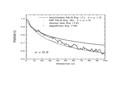
Figure 1: Decay law for the pulse amplitude according to different models. The initial pulse has the form $u(0,t)=\eta_{0}\mbox{sech}(\eta_{0}t)$ with $\eta_{0}=1$. The fiber dispersion randomly varies around $d_{0}=1$ with a mean square fluctuations   $\sigma=0.3$.

Numerical integration of the stochastic NLS Eq.(1) and MF NLS Eq.(6) are performed by the split-step fast Fourier transform. Absorption on the domain boundaries is employed to imitate the infinite length. The system ODE’s Eq.(10), Eq.(11) and Eq.(3) are solved using the procedure DOPRI8 [25], which is based on the Runge-Kutta scheme with adaptive stepsize control.

Inspecting the equation for the field momentum $P$ one can see that $\Omega_{z}=0$. This is due to the fact that the numbers of quanta emitted by the soliton in forward and backward directions are equal. Therefore the predictions of the MFM and IST for $\Omega$ coincide only at the fixed point, where $\Omega=0$. The ratio of amplitudes at the fixed point is $r=\eta_{MFM}/\eta_{IST}\approx 0.97$ for the case of linear amplification, and $r=0.93$ for nonlinear amplification.

The decay of a soliton can be compensated by linear and/or nonlinear amplifications. This results in formation of an autosoliton. In our case, when the pulse power loss due to 4th order dispersion effect $i\gamma u_{tttt}$ is compensated by the linear $i\delta u$ and/or nonlinear $i\mu|u|^{2}u$ amplification in Eq.(1), such an autosoliton can be created. A distinctive property of these solitons is that, they recover the stable waveform when deformed. Fig.2 demonstrates such an aspect of autosolitons, when the power dissipation due to 4th order dispersion term is compensated by linear/nonlinear amplification. Note that the linear amplification gives rise to more pronounced oscillations around the fixed point during transient period compared to nonlinear amplification. At longer propagation distances the oscillations are dumped out and a stable dissipative soliton is formed.

 

Figure 2: Autosoliton acquires its stable form at some propagation distance when its amplitude initially assigned the value greater or lower than corresponding fixed point value $\eta=1.0$. Obtained by numerical solution of the MF NLS Eq.(6) for $\sigma=0.3,\ \gamma=\sigma^{2}/4=0.0225$, with: (a) linear amplification $\delta=0.01,\ \mu=0.0$, and (b) nonlinear amplification $\delta=0.0,\ \mu=0.015.$

The amplitude of the autosoliton at the fixed point can be found from the balance equation (14) of the IST

$$\eta^{2}_{1,2st}=\frac{5\mu}{2\sigma^{2}}\Biggl{(}1\pm\sqrt{1+\frac{6\delta\sigma^{2}}{5\mu^{2}}}\Biggr{)}.$$ (20)

Two types of fixed points exist. The first type $\eta_{1st}$ is defined by the competition between the dissipation (induced by the randomness of the fiber dispersion) and the linear/nonlinear amplifications.

For $\delta=0,\mu>0$ (the nonlinear amplification dominates) we find

$$\eta^{2}_{1st}=\frac{5\mu}{\sigma^{2}},$$ (21)

and similarly for $\mu=0,\delta>0$ (linear amplification dominates)

$$\eta^{2}_{1st}=\sqrt{\frac{15\delta}{2\sigma^{2}}}.$$ (22)

The second type of fixed points is defined by the competition between the linear dissipation and nonlinear amplification.

$$\eta_{2st}\approx\sqrt{\frac{3|\delta|}{2\mu}}-\frac{9|\delta|^{2}\sigma^{2}}{20\mu^{3}},$$ (23)

i.e. the fluctuations reduce the value of amplitude in this case.

The fixed points for the soliton amplitude (at $\sigma=0.3,\delta=0.01,\ \mu=0.015$) as predicted by Eqs.(21), (22) are as follows : $\eta_{1st}=(5\mu/\sigma^{2})^{1/2}\simeq 0.91$, and $\eta_{1st}=(15\delta/2\sigma^{2})^{1/4}\simeq 0.96$. The fixed points of ODE (10) for the same parameters give $\eta=(40\mu/7\sigma^{2})^{1/2}\simeq 0.976$, $\eta=(60\delta/7\sigma^{2})^{1/4}\simeq 0.988$, which is the better approximation to PDE simulation of Fig.2, when we assume that the effect of noise $\sigma$ is accounted by the 4th order dispersive dissipation $\gamma=\sigma^{2}/4$.

Simulations of the stochastic NLS Eq.(1), is presented in Fig.3. Compensation of the damping (due to the randomness of the dispersion) by a linear amplification gives rise to a stable soliton. To verify the property of autolitons observed in Fig.2, we assigned the amplitude greater and lower values, compared to the stationary one $\nu_{st}=1.06$. As expected, the soliton adjusts itself to the stationary amplitude at some propagation distance. Similar behavior is observed when the combination of linear amplification and nonlinear damping is applied (Fig.3b). However, it should be pointed out that the stable pulse propagation is limited by the growth of the zero mode under amplification. When the initial pulse amplitude is close to this solution the instability starts to at distances $z\sim 1/\mu$ (see f.e.[26]).

 

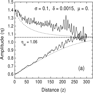
Figure 3: Autosoliton from stochastic NLSE simulations. (a) Evolution of the soliton’s amplitude towards the stationary value as obtained by numerical solution of the stochastic Eq.(1) (solid lines), and as predicted by the ODE model Eq.(10) (dashed lines). Dash-dot line is the stationary value of the amplitude. (b) Autosoliton resulted from the combined effect of a linear amplification and nonlinear dissipation.

The phase trajectories according to Eq.(10) and Eq.(11) is shown in Fig.4. The fixed point appears to be of sink type.

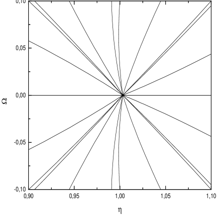
Figure 4: The phase trajectories corresponding to ODE model Eq.(10) and Eq.(11). $\sigma=0.1,\ \delta=0.0015,\ \mu=0.$

Thus, summarizing the results of this section we note, that the optical pulse propagation in fibers with random dispersion can be described as propagation in a uniform fiber with the effective frequency dependent damping. The effect of randomness of the fiber dispersion is accounted by a term with 4th order derivative of the wave envelope. Application of this idea to dispersion-managed solitons will be considered in the next section.

3 Dispersion-managed soliton in a fiber with random dispersion

The dispersion-managed optical communication line consists of fiber sections with alternating anomalous and normal dispersion coefficients [27]. Now the function $d(z)$ is the sum of periodically varying dispersion $d_{0}(z)$ and the random part $d_{1}(z)$ i.e $d(z)=d_{0}(z)+d_{1}(z)$. The usual scale of the DM map is $\sim$ 100 km, so we can consider the random modulations of the dispersion in the white noise limit with $\delta(z)$ correlation. Due to strong variations of the dispersion within the unit cell (the strong dispersion-management regime), locally one has the linear dynamics. The effect of nonlinearity is small in the scale of a unit cell, while accumulated on longer distances, can lead to formation of a breathing DM soliton. Therefore we can expect that the influence of the random modulations of dispersion will result in the frequency dependent damping in the form calculated in the previous section and the nonlinear corrections to this damping will be small.

Performing the averaging over fluctuations yields the following equation

$$iu_{z}+\frac{d_{0}(z)}{2}u_{tt}+|u|^{2}u=-i\gamma u_{tttt}+i\delta u+i\mu|u|^{2}u.$$ (24)

In the case of strong dispersion-management (when $d(z)=(1/\epsilon)d(z/\epsilon),\epsilon\ll 1$, the averaging procedure can be justified [28]. Introducing the variable $\zeta=z/\epsilon$ we obtain the equation

$$iu_{\zeta}+\frac{d(\zeta)}{2}u_{tt}+\epsilon(|u|^{2}-i\delta-i\mu|u|^{2})u=0,$$ (25)

where $d(z)=d_{0}(\zeta)+d_{1}(\zeta),d_{1}\sim\epsilon^{1/2}$. Let us consider the case when $d_{1}\sim\sqrt{\epsilon}$ and thus $d_{1}^{2}\sim\epsilon$. One can decompose the field as $u=<u>+\delta u,\delta u\sim\sqrt{\epsilon}$, and obtain the following estimates for the correction $|\delta u|^{2},\delta u^{2}\sim\epsilon$. Thus, the nonlinear corrections from fluctuations to the averaged equation are of order $\epsilon^{2}$ and can be neglected in comparison with terms $<d_{1}(\zeta)u_{tt}>\sim\epsilon|<u>|^{2}<u>\sim\epsilon$.

The variational approach is proved to be effective for exploring the dispersion-managed soliton [29, 30]. In the presence of nonconservative terms in Eq.(24) we can use the modified variational equations. The equations for the pulse parameters are [31, 32]

$$\frac{\partial L}{\partial\eta_{i}}-\frac{d}{dz}\frac{\partial L}{\partial\eta_{i}}=\int_{-\infty}^{\infty}(R\frac{\partial u^{*}}{\partial\eta_{i}}+c.c.)$$ (26)

Here $L$ is the averaged Lagrangian $L=\int L(z,t)dt$. Employing the Gaussian anzats for the waveform

$$u(z,t)=A(z)\exp[-\frac{t^{2}}{2a(z)^{2}}+i\frac{b(z)t^{2}}{2}+i\phi(z)].$$ (27)

we obtain the following system of ODE’s from the Eq.(26)

$$(a^{2})_{z} = 2d_{0}(z)a^{2}b+6\gamma a^{2}[\frac{1}{a^{4}}-b^{4}a^{4}]-\frac{5}{2\sqrt{2}}\mu A^{2}a^{2},$$

$$(A^{2})_{z} = -d_{0}(z)A^{2}b-\frac{3}{2}\gamma A^{2}[\frac{3}{a^{4}}+2b^{2}-b^{4}a^{4}]+2\delta A^{2}+\frac{13}{4\sqrt{2}}\mu A^{4},$$

$$b_{z} = \frac{d_{0}(z)}{a^{4}}-d_{0}(z)b^{2}-\frac{A^{2}}{\sqrt{2}a^{2}}-12\gamma b(\frac{1}{a^{4}}+b^{2}).$$ (28)

When $\gamma=\delta=\mu=0$, we reproduce the variational equations for a DM soliton [29].

In order to verify the validity of the mean field equation (24) and corresponding variational equations (3) for description of the DM soliton dynamics we compared the result of their numerical solution with that of the original stochastic equation (1), averaged over 50 realisations of random paths. As an initial condition we take the waveform Eq.(27). Parameters of the dispersion map are: $D_{1}=30,\ D_{2}=-28,\ z_{1}=z_{2}=0.078,\ z_{d}=z_{1}+z_{2}$. Fluctuations of the fiber dispersion coefficient is supposed to be of type Eq.(2), and $d(z)=d_{0}(z)[1+\epsilon(z)]$. Satisfactory agreement of these data is displayed in Fig.5.

Figure 5: (a) Comparison of pulse decay rates obtained by numerical integration of the stochastic NLS Eq.(1)  (broken line), the averaged equation Eq.(24)  (solid line), and system of ODE’s (3)  (dashed line). DM map parameters and initial conditions are $D_{1}=30,\ D_{2}=-28,\ z_{1}=z_{2}=0.078,\ z_{d}=0.156,\ A(0)=1.52,\ a(0)=1.059,\ b(0)=0,$ and $\gamma=\sigma^{2}/4,\ \sigma=0.05\div 0.1,\ \delta=\mu=0.$

A characteristic feature of the pulse decay process due to the 4th order dispersion term is that, the pulse amplitude rapidly decreases at initial stage, after that almost linear law is followed. This behavior can be understood from the fact, that $u_{tttt}$ term depends on the pulse shape: its value is bigger when the pulse is more sharp in the initial stage, and becomes small when the pulse is dumped and broadened.

Now we try to compensate the pulse damping due to randomness of the fiber dispersion (which is accounted in the mean field equation as a 4th order derivative term), by linear and/or nonlinear amplification. The Fig.6 demonstrates that this is indeed achievable.

 

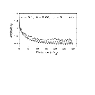
Figure 6: (a) Compensation of the pulse decay by means of linear amplification gives rise to a stable DM soliton: broken line - stochastic NLS Eq.(1), dashed line - ODE (3), solid line - mean field Eq.(24). (b) Combined action of linear and nonlinear amplifications on a longer distance DM soliton propagation. The inset shows the dispersion map (unperturbed -solid line, purturbed - dashed line). DM map parameters and initial conditions are similar to those of figure 5.

An important kind of randomness inherent to real dispersion-managed systems is related to the fluctuations of the lengths of fiber spans $z_{1},\ z_{2}$. In Fig. 7 we illustrate that the decay of a DM soliton due to the randomness of fiber span lengths can be compensated by a suitable linear amplification. Comparison with the non-amplified case ($\delta=0$) shows the effective stabilization of the DM soliton.

 

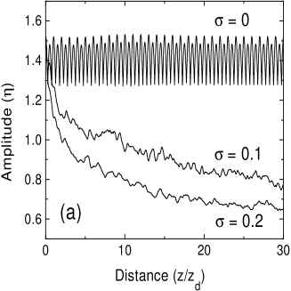
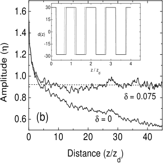
Figure 7: (a) Decay of the amplitude of a DM soliton at different strengths ($\sigma=0\div 0.2$) of fluctuations of the fiber span lengths $z_{1}\cdot(1+\varepsilon(z)),\ z_{2}\cdot(1+\varepsilon(z))$ according to Eq.(1) with $\delta=\mu=0.$ (b) Compensation of the pulse decay (at $\sigma=0.2$) by means of a linear amplification ($\delta=0.075,\ \mu=0$) gives rise to a stable DM soliton. The inset shows the dispersion map (unperturbed -solid line, purturbed - dashed line).

Now let us analyze the fixed points of the system. These points correspond to the stable propagation of a DM soliton under fluctuations of the dispersion map parameters. Equating the left hand sides of Eqs.(3) to zero and assuming $b\sim\delta,\mu,\gamma\ll 1$, we obtain

$$a_{0}^{2} = \frac{\sqrt{2}d_{0}}{A_{0}^{2}},$$ (29)

$$A_{0}^{2} = \frac{2\sqrt{2}\mu d_{0}^{2}}{3\gamma}\Biggl{(}1\pm\sqrt{1+\frac{21\delta\gamma}{4\mu^{2}d_{0}^{2}}}\Biggr{)},$$ (30)

$$b_{0} = \frac{1}{2d_{0}}\Bigl{(}\frac{5\mu A_{0}^{2}}{2\sqrt{2}}-\frac{6\gamma}{a_{0}^{4}}).$$ (31)

According to Eq.(29), the stable DM soliton propagation in optical fibers with random dispersion is possible only in the region of anomalous dispersion ($d_{0}>0$).

4 Conclusion

We have studied analytically and numerically the propagation of optical solitons in fibers with random dispersion. The cases when the unperturbed dispersion is uniform and periodically modulated (DM) are considered. It is shown that the optical pulse dynamics can be successfully described in the framework of the mean field method. The limits of validity of the MFM is revealed by comparison with the results of the perturbation theory, based on the IST. It is shown that when the linear and nonlinear gain/damping are included, corresponding mean field equation coincides with the Swift-Hohenberg equation. Analysis revealed the existence of dissipative solitons in fibers with fluctuating dispersion. The system of variational equations for parameters of the DM soliton has been derived, which takes into account the nonconservative effects due to the randomness of the fiber dispersion. We have analyzed the fixed points of this system and found conditions for the stable propagation of DM solitons in a fiber with gain and fluctuating dispersion. The analytical results are confirmed by direct numerical simulations of the full stochastic NLS equation.

5 Acknowledgements

This work was partially supported by the US CRDF (Award ZM-2095). B.B. thanks the Physics Department of the University of Salerno, Italy, for a two years research grant.

References

- [1] L. F. Mollenauer, P. V. Mamyshev, and M. J. Neubelt, Opt. Lett. 21 (2000) 1274; J. Gripp and L. F. Mollenauer, Opt. Lett. 23 (1998) 1603.
- [2] M. Karlsson, J. Opt. Soc. Am. B15 (1996) 2269.
- [3] F. Kh. Abdullaev, S. A. Darmanyan, A. Kobyakov, and F. Lederer, Phys. Lett. A220 (1996) 213.
- [4] J. Garnier and F.Kh. Abdullaev, Physica D145 (2000) 65.
- [5] C. Xie, L. F. Mollenauer, and N. Mamysheva, J. Lightwave Technol., 21 (2003) 769.
- [6] F. Kh. Abdullaev, J. G. Caputo, and N. Flytzanis, Phys. Rev. E50 (1994) 1552.
- [7] V. I. Karpman, Physica Scripta, 20 (1978) 462.
- [8] D. Kaup, Phys. Rev. A9 (1990) 5689.
- [9] F. Kh. Abdullaev, J. G. Caputo and M.P. Soerensen, in New Trends in Optical Transmission Systems, Ed. A. Hasegawa, Kluwer AP, Dodrecht (1998).
- [10] F. Kh. Abdullaev and B. B. Baizakov, Opt. Lett. 25 (2000) 93.
- [11] B. A. Malomed and A. Berntson, J. Opt. Soc. Am. B18 (2002) 1243.
- [12] F. Kh. Abdullaev, J. Bronski, and G. C. Papanicolaou, Physica D135 (2000) 369.
- [13] T. Schafer, R. Moore, and C.K.R.T. Jones, Opt.Commun. 214 (2002) 353.
- [14] M. Chertkov, I. Gabitov, and J. Moeser, in Nonlinearity and Disorder: Theory and Applications, Eds: F. Kh. Abdullaev, O. Bang, and M. P. Soerensen, Kluwer AP, Dodrecht, 2001.
- [15] M. Chertkov, I. Gabitov, and J. Moeser, Proc. Natl. Acad. Sci. U.S.A. 98 (2001) 14208.
- [16] M. Chertkov, I. Gabitov, P. Luchnikov, J. Moeser, and Z. Toroczkai, J.Opt.Soc.Am. B 19 (2002) 2538.
- [17] M. Chertkov, I. Gabitov, I. Kolokolov, and A. Lebedev, Shedding and Interaction of Solitons in Imperfect Medium, Preprint LANL, 2001;
- [18] After original submission this paper, an article by M. Chertkov et al., Phys. Rev. E 67, (2003) 036615 appeared, where the decay law Eq. (12) was confirmed by means of direct perturbation theory for solitons.
- [19] M. Matsumoto and H. Haus, IEEE Phot. Technol. Lett., 9 (1977) 785.
- [20] K. Blow et al, Techn. Dijest NLGW, OSA Florida (2001).
- [21] V. E. Zakharov, S. V. Manakov, Pisma Zh. Eksp. Teor. Fiz., 70 (1999) 573 [JETP Letters, 70 (1999) 578].
- [22] I. V. Klyatzkin, Stochastic Equations and Waves in Random Media, Nauka, Moscow 1980. (In Russian).
- [23] V. V. Konotop and L. Vazquez, Nonlinear Random Waves, World Scientific, Singapore 1994.
- [24] F. Kh. Abdullaev, Theory of Solitons in Inhomogeneous Media, Wiley, Chichester 1994.
- [25] E. Hairer, S.P. Norsett and G. Wanner, Solving Ordinary Differential Equations I. Nonstiff Problems. 2nd edition. Springer series in computational mathematics, (Springer-Verlag,Heidelberg, 1993).
- [26] N. Akhmediev and A. Ankiewicz, in Spatial Solitons 1, edited by S. Trillo and W.E. Torruelas, Springer-Verlag, Berlin (2000).
- [27] F. M. Knox, N. J. Doran, K. J. Blow, and I. Bennion, Electron. Lett. 32 (1995) 54.
- [28] V. Zharnitsky, E. Grenier, C.K.R.T. Jones, and S.K. Turitsyn, Physica D 152-3 (2001) 794.
- [29] I. Gabitov, S. Turitsyn, Opt. Lett. 21 (1996) 327; I. Gabitov, E. S. Shapiro, and S. K. Turitsyn, Opt. Commun. 134 (1997) 317; S. K. Turitsyn, I. Gabitov, E. W. Ledke, et. al, Opt. Commun. 151 (1998) 117.
- [30] B. A. Malomed, Opt. Commun. 136 (1997) 313.
- [31] A. Bondeson, M. Lisak, and D. Anderson, Phys. Scripta 20 (1979) 479.
- [32] A. Maimistov, Zh. Eksp. Teor. Fiz. 104 (1993) 3620 [JETP 77 (1993) 727].