Fractal dimension of transport coefficients
in a deterministic dynamical system

Abstract

In many low-dimensional dynamical systems transport coefficients are very irregular, perhaps even fractal functions of control parameters. To analyse this phenomenon we study a dynamical system defined by a piece-wise linear map and investigate the dependence of transport coefficients on the slope of the map. We present analytical arguments, supported by numerical calculations, showing that both the Minkowski-Bouligand and Hausdorff fractal dimension of the graphs of these functions is 1 with a logarithmic correction, and find that the exponent $\gamma$ controlling this correction is bounded from above by 1 or 2, depending on some detailed properties of the system. Using numerical techniques we show local self-similarity of the graphs. The local self-similarity scaling transformations turn out to depend (irregularly) on the values of the system control parameters.

1 Introduction

Various transport coefficients associated with a particle moving in low-dimensional periodic array of scatterers are often very irregular functions of control parameters. For example, the diffusion coefficient of a particle moving in the flower-shaped billiard (a 2D Lorentz gas with periodically distributed scatterers of six-petal flower shape) was found to be a very irregular function of the petal curvature [1], and the conductivity of the classical Lorentz gas (with disc scatterers) varies rapidly with the applied field [2]. The reaction rate and the diffusion coefficient in the reaction-diffusion multibaker model also turned out to be irregular, fractal-like functions of the map’s shift [3]. Similar behaviour was found for the diffusion coefficient of a particle thrown onto a periodically corrugated floor and subject to various types of external force, including Hamiltonian [4] and dissipative [5, 6] systems. In chaotic systems with two degrees of freedom the modes governing the relaxation to the thermodynamic equilibrium form a fractal structure with a nontrivial fractal dimension which can be related to the Lapunov exponent and the diffusion coefficient of the system [7, 8, 9]. Another example is provided by a deterministic dynamical system with dynamics defined by iteration of a one-dimensional map: the mean velocity and the drift coefficient in this system were shown to be irregular, nowhere differentiable functions of the system control parameters [10, 11, 12, 13, 14].

It is natural to ask what the origin of these “irregularities” is, how to describe them quantitatively, and to what extent they are universal. Answering all these questions is far from trivial. One of the reasons why irregular behaviour of transport coefficients is so difficult to investigate is that until very recently our knowledge about this phenomenon was based mainly on numerical simulations. Although several different techniques of calculating these quantities were developed, e.g. the transition matrix technique combined with the escape-rate formalism [6, 13, 14, 15, 16, 17, 18], the Green-Kubo formula [6, 14, 15], or the periodic-orbit formalism [15, 19], they all lead to complicated and time-consuming numerical calculations of limited accuracy. Moreover, quite often these techniques are applicable only for some special values of the control parameters. What is worse, as a model becomes more realistic, the results are getting less accurate. For this reason the most precise data have been obtained for very simple, one-dimensional “toy models”, while the question whether a more realistic 2D Lorentz gas (with scatterers of disc shape) exhibits any irregularities in the transport coefficient as functions of the disc radius is still a subject of controversy [6, 20].

This situation improved considerably when Groeneveld and Klages [10] gave exact formulae for the transport coefficients in a simple one-dimensional deterministic dynamical system, introduced by Grossmann and Fujisaka [21], and defined by a piece-wise linear map with two control parameters: the slope and the bias. Their solution has two important features. First, it is complete, i.e. applicable for any (physically meaningful) values of the control parameters. Second, it reduces the problem of determining the transport coefficients to finding the sum of a quickly converging series. For the first time we thus have a model exhibiting irregular behaviour of the transport coefficients, for which a solution permitting an efficient numerical implementation is available.

Klages and Klauß [11] have recently used this exact solution to examine in detail irregular dependency of the drift velocity and diffusion coefficient on the control parameters of the system. Their aim was to verify an earlier hypothesis [12, 13] that the graphs of these quantities as functions of the map slope are so irregular that actually they form fractals. Using two numerical techniques: the box counting and the autocorrelation function methods, they found that the local fractal dimensions of these graphs are well-defined on small finite subintervals, but highly irregular functions of the control parameters. In other words they found that these graphs cannot be described with a single fractal dimension, but rather by a set of quickly varying local fractal dimensions. Taking this into account they put forward a hypothesis that the local fractal dimensions of these graphs as functions of the slope are fractal themselves.

However, our recent numerical calculations [22] suggest that the Minkowski-Bouligand fractal dimension $\Delta$ of the graph of the diffusion coefficient as a function of the slope is equal 1, and that the convergence to this limit is slowed down by a logarithmic correction. Thanks to this logarithmic term the curve is a fractal. We also proposed a conjecture that the exponent controlling this correction depends on the slope of the map and equals either 1 or 2, depending on existence and detailed properties of a Markov partition. That $\Delta=1$ seems to be at odds with the above-cited results of [11], because the Minkowski-Bouligand dimension, if exists, is equivalent to the box-counting dimension [24]. However, one should note that while in our studies we focused on the point-wise dimension calculated only for those system control parameters that correspond to finite Markov partitions, Klages and Klauß computed the box-counting dimension on intervals of finite length, and these two values need not be the same. The aim of our present study is to support our earlier findings analytically. We also present new numerical results that confirm these results.

The structure of the paper is as follows. Section 2 introduces the mathematical formalism. This includes the definition of the model, a brief description of the Minkowski-Bouligand dimension, the “oscillation” method of calculating it for continuous curves, and precise formulation of our hypothesis about the logarithmic corrections. Our main results are contained in section 3, which presents a detailed calculation of the fractal dimension of the graph of the diffusion coefficient as a function of the slope for the case of zero bias. It also includes the derivation of the upper bound for the exponent controlling the logarithmic corrections. Section 4 contains a brief discussion of how our results can be generalized for the case of arbitrary bias and for other transport coefficients. Section 5 contains numerical results. These include analysis of the factors determining the value of the logarithmic correction as well as a study of self-similarity of the graphs. Finally, section 6 is devoted to discussion of results and conclusions.

2 Basic formalism

2.1 The model

Following Groeneveld and Klages [10] we investigate a dynamical system with the equation of motion defined by a one-dimensional map $M_{a,b}\colon\mathbf{R}\to\mathbf{R}$ parameterized by some real numbers $a$ and $b$

$$x_{n+1}=M_{a,b}(x_{n})$$ (1)

where $x_{n}$ represents position of a particle and $n$ is a discrete-time variable. The map is a piece-wise linear function given by

$$M_{a,b}(x)=\left\{\begin{array}[]{l@{\quad:\quad}l}ax+b&x\in[-\textstyle\frac{1}{2},\textstyle\frac{1}{2})\\ M_{a,b}(x+n)-n&x\in\mathbf{R}\end{array}\right.$$ (2)

where $n$ is an arbitrary integer, and the slope $a>1$ and the bias $b\in\mathbf{R}$ are the control parameters of the system (detailed analysis of the system symmetries [10] leads to the conclusion that the values of $b$ can be restricted to $-\textstyle\frac{1}{2}\leq b<\textstyle\frac{1}{2}$). The interval $[-\textstyle\frac{1}{2},\textstyle\frac{1}{2})$ will be called “the fundamental interval” and denoted by $I_{0}^{-}$. However, instead of $I_{0}^{-}$ one can choose $I_{0}^{+}=(-\textstyle\frac{1}{2},\textstyle\frac{1}{2}]$ as the fundamental interval in (2). It turns out that the transport coefficients (defined below) are the same whether we choose $I_{0}^{-}$ or $I_{0}^{+}$ as the fundamental interval. This equivalence has been employed in the derivation of the explicit forms of the transport coefficients [10].

The main features of the dynamical system defined by map $M_{a,b}$ are depicted in figures 1a and 1b. They show $M_{a,b}(x)$ for $a=2.83$ and $b=0.1$ and its action on two initial points $x_{0}$. In particular, figure 1a presents the trajectory of $x_{0}=-\textstyle\frac{1}{2}$ using the fundamental interval $[-\textstyle\frac{1}{2},\textstyle\frac{1}{2})$, while figure 1b shows the trajectory of $x_{0}=\textstyle\frac{1}{2}$ with the fundamental interval $(-\textstyle\frac{1}{2},\textstyle\frac{1}{2}]$. We chose these two trajectories because, as will be explained, they determine all transport properties of the system. The trajectories seem to be rather weakly correlated (which is typical for $b\neq 0$) and “random”. This randomness is related to the fact that, for nearly all values of $a$ and $b$, the iteration of the deterministic map $M_{a,b}$ is equivalent to a stochastic Markov process of a random-walk type [17, 25, 26]: the deterministic trajectory of any point $x_{0}$ can be regarded as a particular realisation of a random-walk process, and taking the average over the initial states $x_{0}$ is equivalent to taking the averages over the corresponding Gibbs ensemble. For this reason the process defined by $M_{a,b}$ (or similar maps) is often called “deterministic diffusion”. The two basic transport coefficients, the drift velocity $J$ and diffusion constant $D$, are defined as

$$J=\lim_{n\to\infty}\frac{\langle x_{n}\rangle}{n},\qquad D=\lim_{n\to\infty}\frac{\langle x_{n}^{2}\rangle-\langle x_{n}\rangle^{2}}{2n},$$ (3)

where $\langle\cdots\rangle$ denotes the average over the uniform ensemble of initial values $x_{0}$. Figure 1 illustrates also the role of using different fundamental intervals. Had we generated both trajectories using the same fundamental interval, they would differ only by a simple translation defined by (2).

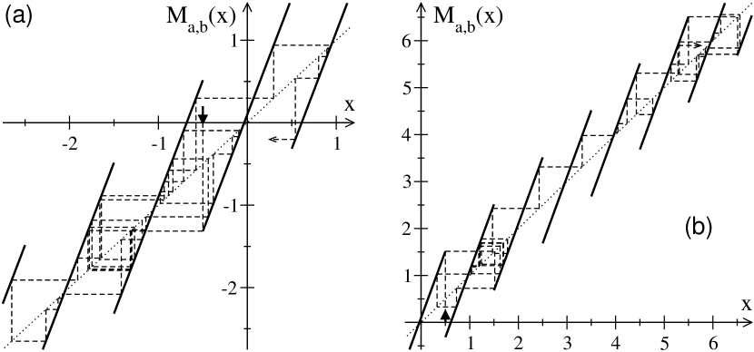
Figure 1: (a) The map $M_{a,b}(x)$ for particular values of the slope $a=2.83$ and the bias $b=0.1$ (thick solid lines); the dashed lines represent the first 33 terms of the trajectory of the point $x_{0}$ under subsequent iterations of $M$ with $x_{0}=-\textstyle\frac{1}{2}$ and the fundamental interval $I_{0}^{-}$. The arrow indicates the initial position $x_{0}$.
(b) The same as in (a), but for $x_{0}=\textstyle\frac{1}{2}$ and the fundamental interval $I_{0}^{+}$. In both cases the transport coefficients are $J\approx 0.128$ and $D\approx 0.0543$.

2.2 Explicit form of the transport coefficients

We will now briefly summarize Groeneveld and Klages’s [10] method of calculating the transport coefficient for the model defined by the map $M_{a,b}$. For each $a>1,b\in\mathbb{R}$, and $\epsilon=\pm$ one can define two infinite sequences of numbers, $y_{r}^{\epsilon}$ and $n_{r}^{\epsilon}$, $r=0,1,\ldots$, consisting of reals and integers, respectively. Their values are uniquely determined by demanding that their first terms are given by

$$y_{0}^{\epsilon}=\frac{\epsilon}{2},\qquad n_{0}^{\epsilon}=0,$$ (4)

and for each $r>0$

$$n_{r}^{\epsilon}+y_{r}^{\epsilon}=ay^{\epsilon}_{r-1}+b,$$ (5)

with additional conditions

$$n_{r}^{\epsilon}\in\mathbb{Z},\quad\textrm{and}\quad y_{r}^{\epsilon}\in I^{\epsilon}_{0}.$$ (6)

Next we define “N-moments”:

$$N_{r}^{\epsilon} = -\frac{\epsilon}{2}+\sum_{s=1}^{r}n_{s}^{\epsilon},$$ (7)

$$N_{k,l}^{\epsilon} = \frac{1}{k!l!}\sum_{r=0}^{\infty}a^{-r}(N_{r}^{\epsilon})^{k}r^{l},$$ (8)

$$N_{k,l} = N^{+}_{k,l}-N^{-}_{k,l},$$ (9)

where $k,l\geq 0$. The basic transport coefficients, $J$ and $D$ can be now expressed ([10], cf. [23]) as

$$J=\frac{N_{2,0}}{N_{1,1}},\qquad D=\frac{N_{3,0}-N_{2,1}J+N_{1,2}J^{2}}{N_{1,1}}.$$ (10)

In the particular case of $b=0$ we have, by symmetry, $J=0$; hence the diffusion coefficient takes on a simpler form

$$D=\frac{N_{3,0}}{N_{1,1}}.$$ (11)

We will also use two important properties derived in Ref. [10]. First

$$N_{1,1}>0,$$ (12)

so that $D$ and $J$ are well-defined for any $a\neq 0$ and $b$. Second, all numbers $n_{r}^{\epsilon}$ are bounded:

$$|n_{r}^{\epsilon}|<\textstyle\frac{1}{2}a+|b|.$$ (13)

2.3 Minkowski-Bouligand fractal dimension of the graph of a continuous function

Let $E$ be a bounded set in the plane. The $\epsilon$-Minkowski sausage of $E$, denoted by $E(\epsilon)$, is the set of all the points whose distance to $E$ is less then $\epsilon$. Let $\mathcal{A}(E(\epsilon))$ be the area of $E(\epsilon)$. Then the Minkowski-Bouligand fractal dimension is defined as [24]

$$\Delta(E)=\lim_{\epsilon\to 0}\left(2-\frac{\log\mathcal{A}(E(\epsilon))}{E(\epsilon)}\right),$$ (14)

provided that this limit exists. In this case it is equivalent to the box-counting dimension [24]. A general relation between the Minkowski-Bouligand dimension $\Delta$ and the Hausdorff dimension $\Delta_{H}$ reads $\Delta\geq\Delta_{H}$. It is conjectured that for all strictly self-similar fractals $\Delta=\Delta_{H}$.

It has been recently proved [10] that the transport coefficients corresponding to the map $M_{a,b}$ are continuous (but not differentiable) functions of the slope $a$ even though $N_{j,k}$ are generally not continuous in $a$. Therefore we can calculate $\Delta$ for the graphs of $D(a)$ or $J(a)$ using the fact that the Minkowski-Bouligand dimension of a continuous real function $f(t)$ defined on an interval $[t_{0},t_{1}]$ can be evaluated through analysis of its Hölder exponents [24] and $\tau$-oscillations [24]. The latter are defined as

$$\textrm{osc}_{\tau}(f;t)=\sup_{|t-t^{\prime}|\leq\tau}f(t^{\prime})-\inf_{|t-t^{\prime}|\leq\tau}f(t^{\prime}).$$ (15)

The Hölder exponents are related to the oscillations as follows. If there exist constants $c>0$ and $0<H\leq 1$ such that for all $\tau$

$$\textrm{osc}_{\tau}(f;t)\leq c\tau^{H}$$ (16)

then $f$ is called a Holderian of exponent $H$ at $t$. If constants $c$ and $H$ are independent of $t$ then the fractal dimension $\Delta$ of $f$ satisfies

$$\Delta\leq 2-H.$$ (17)

Similarly, if there exist constants $c>0$ and $H$ such that for all $\tau$

$$\textrm{osc}_{\tau}(f;t)\geq c\tau^{H}$$ (18)

then $f$ is called an anti-Holderian of exponent $H$ at $t$; if $c$ and $H$ are independent of $t$ then

$$\Delta\geq 2-H.$$ (19)

Relations (17) and (19) constitute a convenient means of calculating the Minkowski-Bouligand dimension $\Delta$. Note that although they are supposed to hold “for all $\tau$”, in practice it suffices to prove their validity only in the limit of $\tau\to 0$.

2.4 Conjecture about the logarithmic correction to the fractal dimension

In [22] we proposed the following conjecture: for the map $M_{a,b}$ in the limit of $\tau\to 0$

$$\frac{\textrm{osc}_{\tau}(D;a)}{\tau}\simeq{\mathcal{C}}(a)\left[-\log(\tau)\right]^{\gamma(a)},\quad\mathrm{with}\;\mathcal{C}(a),\gamma(a)>0.$$ (20)

Together with (15) – (19) this implies that the fractal dimension of the graph of the diffusion coefficient $D$ as a function of the control parameter $a$ is equal 1, but the convergence to this limiting value is logarithmically slow, with the exponent $\gamma$ controlling the convergence rate.

To justify this statement note that since $\lim_{\tau\to 0}(-\log\tau)^{\gamma}/\tau^{H-1}=0$ for any $\gamma\geq 0$ and $H<1$, conjecture (20) implies that $D(a)$ is Holderian of any $H<1$. Using (17) we find that the fractal dimension of its graph is bounded from above by any number of the form $2-H$, with $H<1$. Now we can take the limit of $H\uparrow 1$ to see that $\Delta$ cannot exceed 1. Similarly (20) implies that $D(a)$ is anti-Holderian of exponent $H=1$, and so $\Delta\geq 1$. Hence $\Delta=1$.

In the above analysis we have tacitly assumed that the coefficient $\mathcal{C}(a)$ in (20) can be bounded from below and above by positive constants independent of $a$. We will address this problem in section 5.2.

Since $D$ is a continuous, nowhere differentiable function of $a$ [10], the fractal dimension $\Delta$ must be $\geq 1$ and exponent $\gamma$ must be strictly positive. This reasoning constitutes an alternative derivation of the lower bound for $\Delta$ and explains why $\gamma(a)>0$. Our numerical calculations (performed for the bias $b=0$) indicated that exponent $\gamma$ depends on the slope $a$ and is equal either to 1 or 2, depending on periodicity properties of the sequences $y_{k}^{\pm}$ [22]. In particular, we conjectured that $\gamma=2$ for the slopes $a$ generating disjoint sequences $y_{k}^{+}$ and $y_{k}^{-}$, and $\gamma=1$ otherwise.

Note that even though $\Delta=1$, the graph of $D(a)$ is not an ordinary, smooth curve of dimension 1. Actually, owing to the logarithmic term in (20), this graph is nowhere rectifiable (i.e., any of its arcs is “of infinite length”), which is typical of fractals [24]. Therefore the graph of $D(a)$ locally resembles a well-known family of Takagi functions [6, 14, 15, 24], for their graphs are also nonrectifiable, their dimension is $\Delta=1$, and they satisfy (20) with $\gamma(a)=1$ for all $a$. Takagi functions appear naturally in many contexts related to deterministic diffusion [6, 7, 14, 15].

Since hypothesis (20) opens a convenient way to explore fractal properties of graphs of the diffusion coefficient, its detailed analysis, carried out with both analytical and numerical methods, is one of the main goals of our present paper.

3 Fractal dimension of the diffusion coefficient for $b=0$

In the case of zero bias ($b=0$) the diffusion coefficient $D$ vanishes for the slopes $a\leq 2$. Therefore we shall consider only the nontrivial case of

$$a>2.$$ (21)

The basic properties of the diffusion coefficient are encoded in the sequences $(n_{k}^{\epsilon})$, introduced in Sec. 2.1. Before we will be able to tackle the problem of evaluating the fractal dimension of $D(a)$, we need to derive several useful properties of these sequences.

3.1 Basic properties of $n_{k}$ and $y_{k}$ for $b=0$

3.1.1 Symmetry.

For $b=0$ the sequences $n_{k}^{\pm}$ and $y_{k}^{\pm}$ satisfy

$$n_{k}^{+}=-n_{k}^{-},\qquad y_{k}^{+}=-y_{k}^{-},$$ (22)

so it will suffice to concentrate on the sequences $n_{k}^{+}$ and $y_{k}^{+}$; for simplicity we will denote their terms as $n_{k}$, $y_{k}$, respectively. These sequences may be either periodic or not. Periodic sequences $n_{k}$ (and $y_{k}$) correspond to the so called Markov partitions of the interval $I_{0}^{+}$ (or $I_{0}^{-}$) [13, 14, 17, 25]. Parameters $a$ for which sequences $n_{k}$ and $y_{k}$ are periodic will be called “Markov slopes”. They form a dense set on $(1,\infty)$ [10].

3.1.2 Discontinuity in $a$.

The numbers $n_{k}$, as well as $y_{k}$, can be considered as functions of $a$. Equation (5) implies that all functions $n_{k}(a)$ and $y_{k}(a)$, $k=1,2,\ldots,$ are discontinuous in $a$, which has a profound impact on the functional dependence of the transport coefficients $J$ and $D$ on $a$. This is illustrated in figure 2. Figure 2a presents the quantity of our primary interest: the diffusion coefficient $D$ as a function of the slope $a$ for $4\leq a\leq 6$ and for the vanishing bias $b=0$. Although highly irregular, this function is continuous [10]. One might expect that so are $N_{3,0}(a)$ and $N_{1,1}(a)$, because their quotient equals to $D$. However, as depicted in figures 2b and 2c, actually they are discontinuous. From (7) – (9) we conclude that this must be related to discontinuity of functions $n_{k}^{\pm}(a)$. Two of them, $n_{2}^{+}(a)$ and $n_{3}^{+}(a)$, are shown in figures 2d and 2e, respectively (as horizontal line segments). For completeness, in the same figures are also depicted the graphs of $y_{2}^{+}(a)$ and $y_{3}^{+}(a)$. As expected, there is a clear correlation between discontinuities of $n_{k}(a)$, $y_{k}(a)$ and discontinuities of $N_{3,0}(a)$, $N_{1,1}(a)$. Moreover, there is also a correlation between these discontinuities and “irregularities” of $D(a)$.

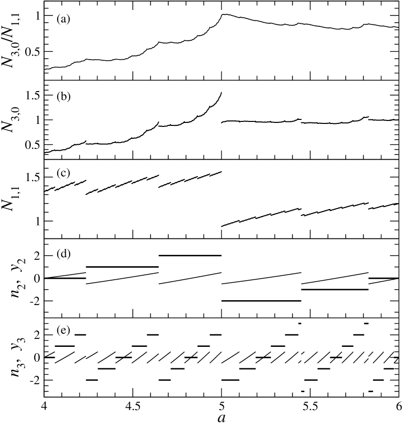
Figure 2: Graphs of the basic quantities used in the mathematical derivation as functions of the slope $a$, calculated for the bias $b=0$. (a) The diffusion coefficient $D=N_{3,0}/N_{1,1}$; (b) $N_{30}$; (c) $N_{11}$; (d) $n_{2}$ (horizontal, thick lines) and $y_{2}$ (thinner curves); (e) $n_{3}$ (horizontal, thick lines) and $y_{3}$ (thinner, almost linear curves). Except for $D$, all of them are discontinuous. $N_{jk}$ are continuous on a dense set $\bar{\Xi}$ and discontinuous on a dense set $\Xi$ which is the union of all discontinuity points of $n_{1}(a),n_{2}(a),n_{3}(a)\ldots$ (see text for details).

The union of all discontinuity points of $n_{k}(a)$ for all $k$ will be denoted by $\Xi$ and we will introduce $\bar{\Xi}$ as the complement of $\Xi$ on the interval $(1,\infty)$. Importance of these two sets is related to the fact that functions $N_{k,l}(a)$ are continuous on $\bar{\Xi}$ and discontinuous on $\Xi$. Moreover, functions $n_{k}(a)$ and $y_{k}(a)$ are also continuous on $\bar{\Xi}$ (however, in contrast to $N_{k,l}(a)$, they can be also continuous on some points of $\Xi$). Both $\Xi$ and $\bar{\Xi}$ are dense on $(1,\infty)$ [10].

3.1.3 Approximate linearity of $y_{k}(a)$.

Figures 2d and 2e suggest that $y_{2}(a)$ and $y_{3}(a)$ consist of almost linear segments even though in reality they are polynomials of degree $2$ and $3$, respectively. Moreover, the density of discontinuity points of $n_{3}$ is considerably greater than that of $n_{2}$. These two important observations can be justified in a more formal way. First of all note that (5) implies

$$y_{k}^{\prime}=y_{k-1}+ay_{k-1}^{\prime}=\sum_{j=0}^{k-1}y_{k-1-j}a^{j},$$ (23)

where we used a short-hand notation $y_{k}^{\prime}=\rmd y_{k}(a)/\rmd a$. Therefore, since $|y_{k}(a)|\leq\textstyle\frac{1}{2}$ and $y_{0}=\textstyle\frac{1}{2}$, the derivative $\rmd y_{k}(a)/\rmd a$ is bounded

$$\frac{a^{k-1}(a-2)+1}{2(a-1)}\leq y_{k}^{\prime}\leq\frac{a^{k}-1}{2(a-1)}.$$ (24)

Taking into account (21) we conclude that for large $k$

$$y_{k}^{\prime}\sim a^{k-1}.$$ (25)

Since the range of each $y_{k}$ is limited to $[-\textstyle\frac{1}{2},\textstyle\frac{1}{2}]$, the distance between two consecutive discontinuity points of $y_{k}(a)$, denoted as $\delta_{k}(a)$, is of order $\lesssim a^{1-k}$, i.e. decreases rapidly with $k$. Similar reasoning leads to the conclusion that the second derivative of $y_{k}(a)$ is of order $\lesssim 2(k-1)a^{k-1}$. Thus the maximal error resulting from truncating the Taylor series of $y_{k}(a)$ after the linear term for the displacement $\delta_{k}(a)\sim a^{1-k}$ is of order $(k-1)/a^{k-1}$ and vanishes quickly as $k$ goes to infinity. Therefore functions $y_{k}(a)$ can actually be approximated to a high accuracy by piece-wise linear segments.

3.1.4 The limits of $a$ going to $a_{0}$ from below and from above.

Although functions $N_{k,l}(a)$ are discontinuous on $\Xi$, they are left continuous. Moreover, it turns out that for any $a_{0}\in(1,\infty)$ the limit of $N_{k,l}(a)$ for $a$ going to $a_{0}$ from above is also well-defined. We will denote it by $\tilde{N}_{k,l}(a_{0})$. Its value can be related to $N_{k,l}(a_{0})$ as follows. For $a_{0}\in\bar{\Xi}$, by definition of $\tilde{\Xi}$, $\tilde{N}_{k,l}(a_{0})=N_{k,l}(a_{0})$. On the other hand, for $a_{0}\in\Xi$ the sequence $n_{0}(a_{0}),n_{1}(a_{0}),\ldots$ is strictly periodic. Denoting the period length by $L$ we thus have $n_{k}(a_{0})=n_{k+L}(a_{0})$ for all $k\geq 0$. For $a$ tending to $a_{0}$ from above the sequence $n_{k}(a)$ will converge to a new sequence $\tilde{n}_{k}(a_{0})$

$$\tilde{n}_{k}(a_{0})=\cases{n_{k}(a_{0}),&$k<L$\\ n_{k}(a_{0})+1,&$k=L$\\ -n_{k}(a_{0}),&$k>L$}$$ (26)

Now $\tilde{N}_{k,l}(a_{0})=\lim_{a\to a_{0}+}N_{k,l}(a_{0})$ can be determined upon substituting $\tilde{n}_{k}(a_{0})$ for $n_{k}$ in (7) – (9). Functions $\tilde{N}_{k,l}(a)$ are right continuous. As argued in [10], all transport coefficients of the system defined by the map $M_{a,b}$ are continuous in $a$. Consequently, functions $\tilde{N}_{k,l}(a_{0})$ can replace $N_{k,l}(a)$ in (10) to calculate the transport coefficients of the system. It is also interesting to note that even though the functions $N_{k,l}(a)$ and $\tilde{N}_{k,l}(a)$ are different, their graphs must be the same. For this reason figure 2b actually shows both $N_{3,0}(a)$ and $\tilde{N}_{3,0}(a)$. Similar conclusion pertains also to figure 2c.

3.2 Oscillations at elements of $\bar{\Xi}$

Let $a_{0}$ be an arbitrary element of $\bar{\Xi}$. This means that all functions $y_{k}(a)$ are continuous at $a_{0}$, and so for each integer $k$ there exists $\varepsilon_{0}>0$ such that $y_{0},y_{1},\ldots,y_{k}$ and $n_{0},n_{1},\ldots,n_{k}$ are continuous and differentiable functions of $a$ on the interval $(a_{0}-\varepsilon_{0},a_{0}+\varepsilon_{0})$. Therefore for any $a\in(a_{0}-\varepsilon_{0},a_{0}+\varepsilon_{0})$ all functions $n_{j}(a)$ up to $j=k$ are independent of $a$. Let $0<\tau<\varepsilon_{0}$. Since $y_{k}(a)$ is continuous on $(a_{0}-\varepsilon_{0},a_{0}+\varepsilon_{0})$, we can write down its Taylor expansion about $a_{0}$ and, following our discussion in section 3.1.3, truncate it after the linear term, obtaining $y_{k}(a_{0}+\tau)\approx y_{k}(a_{0})+\tau y_{k}^{\prime}(a_{0})$.

Let $\mu(\tau;a)$ be the maximum integer $j$ such that $y_{j}(a)$ and $n_{j}(a)$ are continuous on $(a-\tau,a+\tau)$. This means that for any $a_{0}\in\bar{\Xi}$ and a fixed $\mu$ numbers $\mu$ and $\tau$ are related through $y_{\mu}(a_{0})+\tau y_{\mu}^{\prime}(a_{0})\approx\textstyle\frac{1}{2}$ or $y_{\mu}(a_{0})-\tau y_{\mu}^{\prime}(a_{0})\approx-\textstyle\frac{1}{2}$ (whichever gives smaller $\tau$). This, together with (25), leads to the following implicit equation for $\mu(\tau;a)$:

$$\mu(\tau;a)\approx\log_{a}\frac{\textstyle\frac{1}{2}-|y_{\mu(\tau;a)}|}{\tau}.$$ (27)

There are two cases: either the sequence $y_{0}(a_{0}),y_{1}(a_{0}),\ldots$ is periodic (i.e. the system has a Markov partition) or not. In the former case the numerator in (27) is bounded from above and below by positive numbers; in the limit of $\tau\to 0$ we thus have

$$\mu(\tau;a)\approx\log_{a}\tau^{-1}+\mathrm{const}\qquad(\mbox{for }a\in\bar{\Xi}).$$ (28)

Clearly $\mu(\tau;a)\to\infty$ as $\tau\to 0$. In other words, in the limit $\tau\to 0$ (which is essential for the analysis of Hölder exponents), the number of functions in the sequences $y_{k}(a)$ and $n_{k}(a)$ that are continuous on $(a-\tau,a+\tau)$ goes to infinity.

The case where the sequence $y_{0}(a_{0}),y_{1}(a_{0}),\ldots$ is not periodic is far more complicated. The main problem comes from the fact that now the numerator in (27) can get arbitrarily close to zero, which may invalidate (28). In the present approach we restrict ourselves to the cases where the system has a Markov partition and so the sequence $y_{0}(a_{0}),y_{1}(a_{0}),\ldots$ is periodic.

As expressed by (11), the diffusion coefficient is the quotient of two quantities, $N_{3,0}$ and $N_{1,1}$. However, by a straightforward calculation we can verify that for any $\tau>0$ and any functions $f(t)$ and $g(t)$ bounded on $[t-\tau,t+\tau]$ (no matter if continuous or not, but the lower bound for $|g|$ must be $\neq 0$)

$$\textrm{osc}_{\tau}(f/g) = \textstyle\max_{\tau}(f/g)-\min_{\tau}(f/g)$$ (29)

$$\leq \frac{\textrm{osc}_{\tau}(f)\max_{\tau}(g)+\textrm{osc}_{\tau}(g)\min_{\tau}(f)}{\min_{\tau}(g)\max_{\tau}(g)}$$

$$\leq c_{1}\textrm{osc}_{\tau}(f)+c_{2}\textrm{osc}_{\tau}(g)$$

where we used a short-hand notation $\max_{\tau}(f)\equiv\sup_{|t-t^{\prime}|\leq\tau}f(t^{\prime})$ and $\min_{\tau}(f)\equiv\inf_{|t-t^{\prime}|\leq\tau}f(t^{\prime})$, while $c_{1}$ and $c_{2}$ are some nonnegative parameters independent of $\tau$.

Thanks to (12) we can apply (29) to $D(a)$, substituting $N_{3,0}$ for $f$, $N_{1,1}$ for $g$, and $a$ for $t$. The problem of finding the $\tau$-oscillations of the diffusion coefficient $D$ can be thus reduced to that of finding $\textrm{osc}_{\tau}(N_{3,0};a)$ and $\textrm{osc}_{\tau}(N_{1,1};a)$.

Equation (8) implies that for arbitrary integers $k,l$ and $a=a_{0}\pm\tau$

$$N_{k,l}(a_{0})-N_{k,l}(a)\leq\frac{2}{k!l!}\sum_{r=\mu(\tau;a_{0})}^{\infty}\left\{a_{0}^{-r}[N_{r}^{+}(a_{0})]^{k}-a^{-r}[N_{r}^{+}(a)]^{k}\right\}r^{l},$$ (30)

with $\mu$ related to $\tau$ through equation (28). Here we have employed the fact that, by definition of $\mu$, $n_{r}(a)=n_{r}(a_{0})$ and hence $N_{r}^{+}(a)=N_{r}^{+}(a_{0})$ for all $r<\mu(\tau;a)$. Using (13) we conclude that

$$|N_{r}^{+}|\leq c^{*}_{1}r+c^{*}_{2},$$ (31)

with $c_{1}^{*}\geq 0,c_{2}^{*}>0$ being some constants. It will be convenient to assume that $c^{*}_{1}$ denotes the smallest possible value satisfying (31), $c^{*}_{1}\equiv\limsup_{r\to\infty}|N_{r}^{+}(a_{0})|/r$.

Thanks to (31) an upper (as well as lower) bound for $N_{k,l}(a_{0})-N_{k,l}(a)$ can be found by substituting arithmetic sequences for $N_{r}^{+}(a_{0})$ and $N_{r}^{+}(a)$ in (30). Their common differences may be different, but the terms for $r=\mu$ must be the same or differ by a small number less than $\textstyle\frac{1}{2}a+|b|$, cf (13). This leads to

$$|N_{k,l}(a)-N_{k,l}(a_{0})|\lesssim a^{-\mu}\mu^{k+l-1}, \qquad\textrm{for }c^{*}_{1}>0,$$ (32)

$$|N_{k,l}(a)-N_{k,l}(a_{0})|\lesssim a^{-\mu}\mu^{l}, \qquad\textrm{for }c^{*}_{1}=0.$$ (33)

This important result can be also obtained by noticing that the major contribution to the sum in (30) comes from its first few terms. Hence, using (28),

$$|N_{k,l}(a_{0}\pm\tau)-N_{k,l}(a_{0})|\lesssim\tau\ln^{k+l-1}(\tau^{-1}), c_{1}^{*}>0,$$ (34)

$$|N_{k,l}(a_{0}\pm\tau)-N_{k,l}(a_{0})|\lesssim\tau\ln^{l}(\tau^{-1}), c_{1}^{*}=0,$$ (35)

which implies

$$\textrm{osc}_{\tau}(N_{k,l};a)\lesssim\tau\ln^{k+l-1}(\tau^{-1}), c_{1}^{*}>0,$$ (36)

$$\textrm{osc}_{\tau}(N_{k,l};a)\lesssim\tau\ln^{l}(\tau^{-1}), c_{1}^{*}=0.$$ (37)

Consequently, by (29) and (11),

$$\textrm{osc}_{\tau}(D;a)\lesssim\tau\ln^{2}(\tau^{-1}), \qquad c_{1}^{*}>0,$$ (38)

$$\textrm{osc}_{\tau}(D;a)\lesssim\tau\ln(\tau^{-1}), \qquad c_{1}^{*}=0.$$ (39)

for all $a\in\bar{\Xi}$.

Equations (38) and (39) give the upper bound for the exponent $\gamma$ controlling the logarithmic correction to the local fractal dimension. As we can see, this upper bound depends on $c^{*}_{1}$. This constant has a simple physical interpretation. If the trajectories of points $x_{0}=\pm\textstyle\frac{1}{2}$ under $M_{a,b}$ (like those depicted in figure 1) remain confined inside a neighborhood of the origin, we can take $c^{*}_{1}=0$, which implies $0<\gamma\leq 1$. Otherwise $c^{*}_{1}>0$ and $0<\gamma\leq 2$.

3.3 Oscillations at elements of $\Xi$

The argumentation presented in section 3.2 might seem of little use for elements of the set $\Xi$, at which functions $N_{k,l}(a)$ are discontinuous. However functions $N_{k,l}(a)$ are left continuous and have a well-defined limit from the right, $\tilde{N}_{k,l}(a)$. Functions $\tilde{N}_{k,l}(a)$ are right continuous and, as argued in section 3.1.3, can replace $N_{k,l}(a)$ in calculations of the transport coefficients. This suggests a method of circumventing the problems related to discontinuity. The oscillation of the diffusion coefficient $D$ on the interval $[a_{0}-\tau,a_{0}+\tau]$ with $a_{0}\in\Xi$ can be calculated as the maximum of two values: the oscillation of $(N_{3,0}/N_{1,1})(a)$ on $[a-\tau,a]$ and the oscillation of $(\tilde{N}_{3,0}/\tilde{N}_{1,1})(a)$ on $[a,a+\tau]$. In each case we can now apply the reasoning of section 3.2 (its most delicate point, validity of approximation (28), can be justified rigorously because the sequence $n_{k}(a)$ is periodic for all $a\in\Xi$). This implies that (38) and (39) are valid also for all $a\in\Xi$, which suggests that the fractal dimension of the diffusion coefficient is 1 for all Markov slopes $a\in(1,\infty)$.

4 The case $b\neq 0$

Besides the fractal properties of the diffusion coefficient $D$, in the asymmetric case $b\neq 0$ we can investigate also those of the drift $J$, which for $b\neq 0$ is also a highly irregular function of the control parameters [10]. It turns out that the methods developed in section 3 can be readily extended to the case of nonvanishing bias $b$ and to the analysis of arbitrary transport coefficients. Therefore we will only discuss the major differences and difficulties appearing when applying these methods to the more general case $b\neq 0$.

First, although derivation of the basic relation (27) remains practically unchanged, we see that restricting our calculations to the case $1<a\leq 2$ is fully acceptable only for $b=0$. This is related to the fact that for $b\neq 0$ the transport coefficients can assume nontrivial values also for $a\leq 2$ [10], so this parameter region also deserves attention. The assumption $a>2$ greatly simplifies the proof of (25) (cf. (24)); without it we have to take into account correlations between consecutive terms of the sequences $y_{k}^{\pm}$. Our numerical analysis shows that (24), and hence (27), is valid also for $1<a\leq 2$ (at least in the limit of $k\to\infty$), but we failed to find a rigorous proof of it.

Second, the sequences $n_{k}^{+}$ and $n_{k}^{-}$ are no longer related to each other by (22) and in practice must be considered as independent of each other. This, fortunately, is not a serious difficulty – actually relation (22) was used mainly to simplify notation.

Third, just as in the case $b=0$, we can justify transition from (27) to (28) only in the case where both $n_{k}^{+}$ and $n_{k}^{-}$ are periodic, i.e. when the system has a Markov partition.

Fourth, we still need an analytical argument justifying our claim that the graph of $(D;a)$ is uniformly anti-Holderian for all $b$.

Although in section 3 we focused on the fractal properties of the diffusion coefficient $D$, our analysis was as general as possible. In particular inequalities (36) and (37) were derived for functions $N_{k,l}(a)$ with arbitrary $k,l$. Since all transport coefficients, including the drift velocity $J$, can be expressed as functions of the quotients $N_{k,l}/N_{1,1}$ [10], the methods of section 3 can be applied for arbitrary transport coefficients.

Consequently, we can follow the ideas of section 3 to argue that the local fractal dimension of the graphs of transport coefficients as functions of $a$ is 1 for the control parameters $a$ and $b\in\mathbb{R}$ such that $a>2$ and the system has a Markov partition. Based on our numerical calculations [22] and heuristic arguments we conjecture the same fractal behaviour for all other pairs $(a,b)$.

5 Numerical results

5.1 The role of $c^{*}_{1}$

Equations (38) and (39) imply that the exponent $\gamma$ controlling the logarithmic correction is bounded from above by 2 for $c^{*}_{1}>0$ and by 1 for $c^{*}_{1}=0$. On the other hand, however, in [22] we conjectured that the value of $\gamma$ depends on properties of the periods of sequences $y_{k}^{+}$ and $y_{k}^{-}$ (i.e., whether they consist of the same or different terms). A question arises whether the two approaches lead to the same conclusions for $\gamma$ and if not, what does its value really depend on?

To answer it we will study a particular case of the bias $b=0$ and the slope $a$ equal to the largest root of $a^{5}-2a^{4}-2a^{3}+2a^{2}+1$, i.e. $a\approx 2.455$. The trajectory of $x_{0}^{+}=\textstyle\frac{1}{2}$ is $x_{1}^{+}\approx 1.23,x_{2}^{+}\approx 1.56,x_{3}^{+}\approx 0.92,x_{4}^{+}\approx 0.80,x_{5}^{+}=x_{0}^{+},\ldots$, and so the sequence $x^{+}_{m}$ is periodic, $x_{5+m}^{+}=x_{m}^{+}$. The trajectory of $x_{0}^{-}$ is given by $x_{m}^{-}=-x_{m}^{+}$, and hence is periodic, too. Since all terms of the sequence $x_{k}^{-}$ are different from those of $x_{k}^{+}$, according to [22] the value of $\gamma$ should be 2. This is in conflict with (39), as the trajectories of $x_{0}=\pm\textstyle\frac{1}{2}$ are bounded, hence $c^{*}_{1}=0$ and, following (39), $\gamma\leq 1$. We checked this numerically using the arbitrary precision arithmetic library GMP [27]. Our results are presented in figure 3. It clearly suggests that $\gamma=1$. This implies that our earlier hypothesis about the logarithmic correction exponent $\gamma$ was incorrect. Our present, deeper insight into mathematical nuances of the problem leads to the conclusion that the main factor determining the value of $\gamma$ (at least for systems with periodic trajectories of $x_{0}=\pm\textstyle\frac{1}{2}$) is whether the constant $c^{*}_{1}$ vanishes or not.

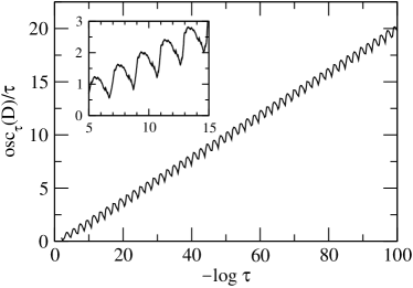
Figure 3: Oscillations of the diffusion coefficient $D$ for $b=0$ and $a$ equal to the largest root of $a^{5}-2a^{4}-2a^{3}+2a^{2}+1$, i.e. $a\approx 2.455$, rescaled in accordance with (20) and calculated on intervals $(a-\tau,a+\tau)$ for $10^{-100}\leq\tau\leq 10^{-2}$. The inset presents a blowup of the results and reflects periodicity of the curve.

Figure 3, and especially the inset in it, indicates also that in the case of the map $M_{a,b}$ oscillations of the diffusion coefficient really deserve their name. Apparently the graph of $\textrm{osc}_{\tau}(D)/\tau$ as a function of $\log\tau^{-1}$ is a composition of a linear and periodic, “oscillating” function. The period length $\lambda$ of these “oscillations of oscillations” can be estimated using (28),

$$\lambda=a^{L},$$ (40)

where $L$ is the period of $y_{k}^{\pm}$; in our case $L=5$, $\lambda=a^{5}\approx 89$, $\log\lambda\approx 1.95$, in excellent agreement with the data in figure 3.

5.2 The uniformly Hölder and anti-Hölder conditions for $D(a)$

As we explained in section 2.4, analysis of Hölder exponents can be useful in exploration of fractal properties of a curve if this curve is uniformly Holderian (or anti-Holderian), i.e. if the coefficient $\mathcal{C}(a)$ in (20) can be bounded from below (or above) by a constant number. We decided to check these properties numerically for the vanishing bias $b$, as in this particular case all Markov slopes $a$ are algebraic numbers. They can be thus generated in a systematic way by first generating polynomials with integer coefficients and then identifying Markov slopes with the largest roots of the polynomials. Moreover, the coefficients of each such polynomial determine the numbers $n_{r}^{\epsilon}$, hence whether the constant $c_{1}^{*}$ vanishes or not, and thus whether the exponent $\gamma(a)$ in our conjecture (20) is expected to equal 1 or 2, respectively.

To check whether $D(a)$ is uniformly anti-Holderian we concentrated on the case $\gamma(a)=1$, i.e. $c_{1}^{*}=0$. Using a computer program we found all Markov slopes $a\in(2;8]$ that are algebraic numbers of degree $d\leq 4$ and correspond to $c_{1}^{*}=0$. Then, for each such a slope, we calculated the coefficient $\mathcal{C}(a)$. To this end we assumed that at each investigated slope the graph of $\mathrm{osc}_{\tau}(D;a)$ as a function of $\log\tau^{-1}$ behaves like the one depicted in figure 3. To increase accuracy we eliminated local periodic oscillations of the curves by using (40). As expected, the points of each curve at abscissas forming an arithmetic sequence with a common difference $\log\lambda$ turned out to form practically a straight line with the slope quickly converging; we identified this limiting slope with $\mathcal{C}(a)$. In each case the sum of squares of the residuals from the best-fit line was less than $10^{-10}$. The results obtained in this way are depicted in figure 4a. As expected, the density of the points increases with $a$. Moreover, apparently they lie on a continuous curve that crosses the $x$-axis only at $a=2$. These findings are supported by the results depicted in the inset of this figure and obtained for all Markov slopes $a\in(2;3]$ that correspond to $c_{1}^{*}=0$ and $d\leq 6$. That $\mathcal{C}(a)$ tends to a continuous curve implies that the graph of $D$ as a function of $a$ is uniformly anti-Holderian with $H=1$ and $\gamma=1$ at least on the set of all Markov slopes $a>2$ for which $c_{1}^{*}=0$. Note that this set is dense on $(2,\infty)$.

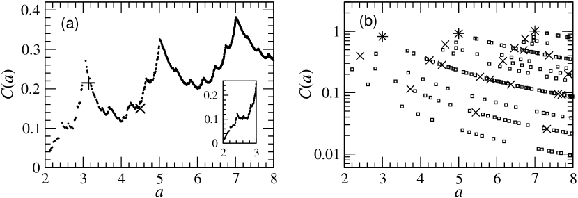
Figure 4: (a) The coefficient $\mathcal{C}(a)$ for all Markov slopes $a\in(2;8]$ that correspond to $\gamma=1$ and are algebraic numbers of degree $d\leq 4$ (2054 data points). The inset presents the same quantity calculated for $a\in(2;3]$ and $d\leq 6$ (439 data points). The plus ($+$) and cross ($\times$) signs mark the estimated values of $\mathcal{C}(a)$ for non-Markov slopes $a=\pi$ and $a=4.5$, respectively. (b) The same as in (a), but for $\gamma=2$ and $d=1$ (stars), $d=2$ (crosses), and $d=3$ (small squares). The logarithmic scale for the ordinate axis was used to visualize the structure of $\mathcal{C}(a)$.

To check whether $D(a)$ is uniformly Holderian we focused on the Markov slopes with $\gamma(a)=2$, i.e., $c_{1}^{*}\neq 0$. We investigated numerically all Markov slopes $a\in(2;8]$ that are algebraic numbers of degree $d\leq 3$ and correspond to $c_{1}^{*}\neq 0$ (286 data points). We found that at each such a slope the exponent $\gamma$ is actually equal to 2. However, as seen in figure 4b, the coefficient $\mathcal{C}(a)$ turned out to be a highly irregular, discontinuous function of $a$. Fortunately, this function is apparently bounded from above. Taking into account our earlier result for $c_{1}^{*}=0$, we conclude that the graph of the diffusion coefficient $D$ as a function of the slope $a$ is uniformly Holderian (with $H=1$ and $\gamma=2$) at least on the (dense) set of all Markov slopes.

The analysis of the Hölder and anti-Hölder condition at non-Markov slopes is far more difficult. Such values of $a$ were already investigated numerically in [22]. The conclusion was that in this case most probably $\gamma=1$, but this property cannot be definitely established numerically due to very poor convergence. In several cases there is a clear linear trend in graphs of $\mathrm{osc}_{\tau}(D;a)$ as a function of $\log\tau^{-1}$, which permits to estimate the value of $\mathcal{C}(a)$ (assuming $\gamma(a)=1$). For example, using the data of [22], we can estimate $\mathcal{C}(\pi)\approx 0.215$ and $\mathcal{C}(4.5)\approx 0.15$. As seen in figure 4, these values are very close to those obtained for the nearby Markov slopes. However, for many other values of $a$ no reasonable numerical estimation of $\mathcal{C}(a)$ is possible.

5.3 Oscillations of $N_{k,l}(a)$

Results of section 3.2 reveal that the logarithmic corrections to fractal dimensions of graphs of transport coefficients must be attributed to similar logarithmic corrections in functions $N_{k,l}(a)$. For $a\in\tilde{\Xi}$ these latter functions are continuous in $a$ and we expect them to satisfy (20) with $N_{k,l}$ substituted for $D$, i.e., for $\tau\to 0$

$$\frac{\textrm{osc}_{\tau}(N_{k,l};a)}{\tau}\sim\left[\log(\tau^{-1})\right]^{\gamma_{k,l}(a)}$$ (41)

where, following (36) and (37),

$$0\leq\gamma_{k,l}\leq k+l-1 \textrm{for }c_{1}^{*}>0,$$ (42)

$$0\leq\gamma_{k,l}\leq l \textrm{for }c_{1}^{*}=0.$$ (43)

This conjecture relates the fractal nature of transport coefficients to fractality of functions $N_{k,l}(a)$ which—although of no immediate physical meaning—have much simpler form and are more amenable to rigorous treatment.

To verify (41) – (43) we have calculated oscillations of $N_{3,0}$ and $N_{1,1}$ for the vanishing bias $b$ and two values of the slope $a$: the largest root of $a^{5}-4a^{4}+2a^{3}+3a^{2}-2a+4$ (i.e., for $a\approx 3.04$) and the largest root of $a^{5}-4a^{4}-4a^{2}+a+4$ (i.e., for $a\approx 4.20$). For these parameter values the system has a Markov partition [22]; moreover, the constant $c^{*}_{1}=0$ for $a\approx 3.04$ and $c^{*}_{1}>0$ for $a\approx 4.20$.

Our results for $a\approx 3.04$ and $a\approx 4.20$ are depicted in figures 5a and 5b, respectively. As we can see, our data clearly indicate that in both cases $\gamma_{1,1}=1$. However, $\gamma_{3,0}=0$ in figure 5a (i.e., for $c^{*}_{1}=0$) and $\gamma_{3,0}=2$ in figure 5b (i.e., for $c^{*}_{1}>0$). All these results are in perfect agreement with (43) and actually correspond to the upper bounds implied by these equations. Note that for $c^{*}_{1}=0$ equation (43) actually gives not only the upper bound, but the exact value of $\gamma_{k,0}=0$ for all $k>0$.

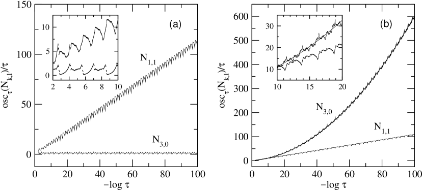
Figure 5: Oscillations of $N_{1,1}$ and $N_{3.0}$ rescaled in accordance with (41) calculated on intervals $(a-\tau,a+\tau)$ for $10^{-100}\leq\tau\leq 10^{-2}$, with $b=0$ and $a$ equal to the largest root of (a) $a^{5}-4a^{4}+2a^{3}+3a^{2}-2a+4$, (b) $a^{5}-4a^{4}-4a^{2}+a+4$. Results for $N_{3,0}$ in the right panel were fitted by a quadratic (a solid line, hardly distinguishable from numerical data). The insets are blowups of the curves to show their periodicity and discontinuity in $a$.

The insets in figure 5 suggest that, just as in the case of graphs of $\textrm{osc}_{\tau}(D)/\tau$ discussed in section 5.1, on finer scales the graphs of $\textrm{osc}_{\tau}(N_{k,l})/\tau$ as functions of $\log\tau^{-1}$ have periodic components. Their period lengths $\lambda$ can be calculated using (28), which gives $\lambda=a^{6}\approx 794$ for $a\approx 3.04$ (figure 5a) and $\lambda=a^{4}\approx 311$ for $a\approx 4.20$ (figure 5b). These theoretical values are in excellent agreement with numerical data used to produce figure 5.

5.4 Self-similarity of the graphs

In the limit of $\tau\to 0$ the periodicity of the curves presented in figures 3 and 5 becomes practically perfect. This phenomenon could be a consequence of local self-similarity of functions $D(a)$ and $N_{k,l}(a)$ under enlargement of their graphs by a scale factor $\lambda$. To verify this hypothesis in figure 6a we have plotted the graph of the diffusion coefficient $D$ as a function of the slope $a$, with the origin moved to the point $a_{0}\approx 2.455$ and $D_{0}\equiv D(a_{0})\approx 0.0967$. Then we plotted three consecutive blowups of this graph obtained by magnifying it about the new origin by scale factors $\lambda$, $\lambda^{2}$, $\lambda^{3}$, where $\lambda=a_{0}^{5}\approx 89$. As we can see in figure 6a, this simple transformation of graphs does not lead to perfectly self-similar structures; nevertheless, the curves thus obtained do exhibit some kind of similarity.

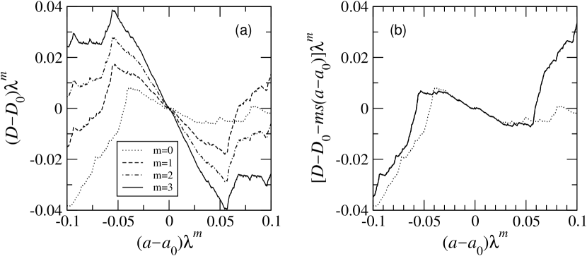
Figure 6: (a) The graph of the diffusion coefficient obtained for the slope $a_{0}\approx 2.455$ and the bias $b=0$ (dotted line) and its consecutive $\lambda$-fold magnifications about the point $(a_{0},D_{0})$, where $\lambda=a_{0}^{5}\approx 89$ and $D_{0}\equiv D(a_{0})\approx 0.0967$. (b) The same as in (a), except that now each $\lambda$-fold magnification has been followed by a linear transformation $(x,y)\mapsto(x,y-sx)$ with $s\approx-0.1969$; all 4 curves have been plotted, but those obtained for $m=1,2,3$ differ from each other by less than the line width.

The effect of actual self-similarity can be achieved if each $\lambda$-fold enlargement will be followed by a correction transformation related to the nonvanishing logarithmic correction exponent $\gamma$. The 2-step transformation $T$ can be expressed as

$$T(x,y)=(\lambda x,\lambda y-\kappa_{1}(\lambda x)),$$ (44)

where $\lambda$ is the scale factor and $\kappa_{1}$ is a correction term. Our numerical results suggest that for $\gamma=1$ this complementary step is a simple linear transformation, $\kappa_{1}(x)=sx$, with $s$ being a constant depending on the slope $a$, the bias $b$ and the function the self-similarity transformation $T$ is applied to. In the case of the data shown in figure 6 the constant $s\approx-0.1969$. The net effect of this two-step scaling procedure applied iteratively $m=0,1,2,3$ times is depicted in figure 6b. As we can see, the convergence is very fast and the curves obtained after $m=$ 1, 2 and 3 elementary 2-step transformations are already practically indistinguishable from each other. Closer analysis of the numerical data for $m=0,\ldots,10$ revealed that with each 2-step transformation we get closer to the self-similar limit curve by about two significant figures. Similar behaviour was found for several other points $a_{0}$, both for graphs of the diffusion coefficient $D(a)$ and the auxiliary functions $N_{1,1}(a)$, $N_{3,0}(a)$, provided that the corresponding logarithmic correction exponent $\gamma$ was 1. Note that transformation of type (44) holds also for Takagi functions.

For $\gamma=1$ the net effect of applying consecutively $m$ transformation $T$ is

$$T_{m}(x,y)=(\lambda^{m}x,\lambda^{m}y-m\kappa_{1}(\lambda^{m}x)),$$ (45)

where linearity in $m$ of the correction term corresponds to $\gamma=1$. For $\gamma=2$ the situation gets more complicated. We now expect that the correction term after $m$ self-similarity transformations is quadratic in $m$,

$$T_{m}(x,y)=(\lambda^{m}x,\lambda^{m}y-m^{2}\kappa_{2}(\lambda^{m}x)-m\kappa_{1}(\lambda^{m}x)),$$ (46)

with some real functions $\kappa_{1}$ and $\kappa_{2}$. A side-effect of such a form of the correction term is that, in contrast to the case $\gamma=1$, now the second step in each elementary 2-step transformation depends on $m$ and hence slightly differs from each other. We have confirmed (46) numerically, finding the convergence to be very fast. In particular, figure 7 presents results obtained for the slope $a_{0}\approx 4.20$ and bias $b_{0}=0$ (these parameters were already used in figure 5b). On the left panel we show correction functions $\kappa_{1}$ and $\kappa_{2}$. As we can see, $\kappa_{2}$ is linear, while $\kappa_{1}$ is an irregular (perhaps fractal) function of its argument. Although the graph of $\kappa_{1}(x)$ in figure 7a is quite similar to that of $D(a)$ (dotted line in figure 7b), these two functions are different. On the right panel we present effects of applying $T_{m}$, $m=0,1,2,3$, to the graph of $D(a)$ in the vicinity of the point $(a_{0},D(a_{0}))$. The convergence to the self-similar limit is very fast. Actually for $m>1$ the graphs of $T_{m}$ in figure 7b differ from each other by less than the line width.

Figure 7: (a) Correction functions $\kappa_{1}$ and $\kappa_{2}$ used in self-similarity transformation (46) for the graph of the diffusion coefficient $D(a)$ about the point ($a_{0},D_{0})$ with $a_{0}\approx 4.20$, $D_{0}=D(a_{0})$, and the bias $b=0$. (b) The self-similarity effect of applying $T_{m}$, as described by (46), to the graph of $D(a)$, for the same parameter values as those used to generate panel (a). Note that the dotted line (corresponding to $m=0$) actually represents the graph of the original function $D(a)$ translated by a vector $(-a_{0},-D_{0})$ and $x$ can be interpreted as $\lambda^{m}(a-a_{0})$. The graphs obtained for $m\geq 1$ are practically indistinguishable from each other.

6 Summary and conclusions

We have analysed both analytically and numerically the local (Minkowski-Bouligand) fractal dimension of graphs of transport coefficients as functions of the slope $a$ in a simple dynamical system defined by a piece-wise linear map $M_{a,b}$. We showed that for all values of the control parameters $a$ and $b$ such that the system defined by $M_{a,b}$ has a Markov partition, the dimension of such graphs is 1, probably with a logarithmic correction. This correction renders the curves nowhere rectifiable (i.e., any of their arcs is “of infinite length”), which is typical of fractals. Our results imply also that the Hausdorff dimension of these curves is 1, too.

We have also found the upper bound for the exponent $\gamma$ controlling the logarithmic correction. This bound turned out to be either 1 or 2, depending on whether a constant $c^{*}_{1}$ vanishes or not, or, equivalently, whether the trajectories of $x_{0}=\pm\textstyle\frac{1}{2}$ remain bounded or not. This finding extends our earlier conjecture [22] about factors determining the value of $\gamma$.

Using numerical calculations we have shown that at Markov slopes $a$ the graph of the diffusion coefficient is actually self-similar under the action of a special, two-step scaling transformation. The first step is a simple uniform enlargement by a scale factor $\lambda$. This transformation must be followed by the second step, a “correction” transformation of the graph, which is related to the non-zero value of the exponent $\gamma$ controlling the logarithmic correction to the local fractal dimension. We found the precise formula for the value of the scale factor $\lambda$ as well as a general form of the correction transformations. In particular, we found that the scale factor $\lambda$ depends on the slope $a$ and the periodicity of the trajectories of points $x_{0}=\pm\textstyle\frac{1}{2}$. The correction transformations turned out linear (affine) for $\gamma=1$ and different, more complicated for $\gamma=2$. At non-Markov slopes the graphs are probably not self-similar.

The graphs of transport coefficient have thus surprisingly reach spectrum of local fractal properties. Our numerical results suggest that the curves are self-similar on a dense set of points (at which the system has a Markov partition), but at each such a point the scale factor and the correction transformation are different. In this sense the curves are multifractals.

Our analytical approach has, however, some limitations. The most serious one is related to the fact that it is applicable only to systems in which the trajectories of points $x_{0}=\pm\textstyle\frac{1}{2}$ are periodic (or, equivalently, to systems with a Markov partition). We believe that the typical value of $\gamma$ at non-Markovian slopes $a$ is 1, but in general this value can take on any value between 1 and 2. This conjecture, however, requires further studies. Proving that the investigated curves are uniformly Holderian with $H=1$ and $\gamma=2$ and anti-Holderian with $H=1$ and $\gamma=1$ is another open problem. So far we have been able to justify these properties only numerically.

Numerical results suggest that our analytical approach gives not only the upper bound, but the exact value of $\gamma$. To prove this hypothesis rigorously would require finding a “tight” lower bound for $\gamma$. However, as is well known [24], finding the lower bound of a fractal dimension is usually much more difficult that finding the upper one. This is also true in our case. For example, when we were looking for the upper bound of oscillations of the quotient of two functions, we did not have to take into account the fact that actually their values were correlated. Applying the same general assumption for the lower bound of $\gamma$ yields only a trivial result $\gamma\geq 0$. Therefore finding a better lower bound for the logarithmic correction is another problem for future studies.

Another question is how to reconcile our results with those obtained by Klages and Klauß [11], who analysed the box-counting dimension of $D(a)$ on intervals of finite length and found it to be greater than 1. One possible way of answering this problem could be to analyse how the local self-similarity of the curves depends on the box size.

Although most of our analysis was carried out explicitly for the graph of the diffusion coefficient $D$ as a function of the slope $a$ for a vanishing bias $b$, we showed how it can be generalized for other transport coefficients and for arbitrary bias $b$. Similarly we expect that the main conclusions derived here for the simple piece-wise linear map $M_{a,b}$ remain valid also in the case of more realistic (and complex) dynamical systems. After all, in our model the main reason for irregular, fractal dependence of the transport coefficients on the slope $a$ is an extreme sensitivity of the (periodic) Markov orbits on the control parameters; similar sensitivity is observed in more complex models, e.g. the multiBaker or the Lorentz gas [1, 2, 3, 6, 17]. Transport coefficients in these models were already called ”fractal”, but only in the sense of ”unexpectedly irregular”. We hope that our present approach will help justifying a conjecture that the transport coefficients in those more realistic models form fractals in a strictly mathematical sense of this term.

References

References

- [1] Harayama T Klages R and Gaspard P 2002 Phys. Rev. E 66 026211
- [2] Lloyd J et al1995 Chaos 5 536
- [3] Gaspard P and Klages R 1998 Chaos 8 409
- [4] Harayama T and Gaspard P 2001 Phys Rev. E 64 036215
- [5] Mátyás L and Klages R 2004 Physica D 187 165
- [6] Klages R 2003 Microscopic Chaos, Fractals, and Transport in Nonequilibrium Steady States (Dresden: Max Planck Institut, habilitation thesis)
- [7] Gilbert T Dorfman J R and Gaspard P 2001 Nonlinearity 14 339
- [8] Gaspard P Claus I, Gilbert T and Dorfman J R 2001 Phys. Rev. Lett. 86 1506
- [9] Claus I and Gaspard P 2002 Physica D 168 266
- [10] Groeneveld J and Klages R 2002 J. Stat. Phys. 109 821
- [11] Klages R and Klauß T 2003 J. Phys. A: Math. Gen. 36 5747
- [12] Klages R and Dorfman J R 1995 Phys. Rev. Lett. 74 387
- [13] Klages R and Dorfman J R 1999 Phys. Rev. E 59 5361
- [14] Klages R 1996 Deterministic Diffusion in One-Dimensional Chaotic Dynamical Systems (Berlin: Wissenschaft und Technik Verlag)
- [15] Dorfman J R 1999 An Introduction to Chaos in Nonequilibrium Statistical Mechanics (Cambridge: Cambridge University Press)
- [16] Gaspard P and Nicolis G 1990 Phys. Rev. Lett. 65 1693
- [17] Vollmer J 2002 Phys. Rep. 372 131
- [18] Gaspard P 1992 J. Stat. Phys. 68 673
- [19] Cvitanović P et al2003 Chaos: classical and quantum (Copenhagen: Niels Bohr Insitute, http://www.nbi.dk/ChaosBook/)
- [20] Klages R and Dellago Ch 2000 J. Stat. Phys. 101, 145.
- [21] Grossmann S and Fujisaka H 1982 Phys. Rev. A 26 1779
- [22] Koza Z 2004 Acta Phys. Polon. B 35 1365
- [23] Koza Z 1999 J. Phys. A: Math. Gen. 32 7637
- [24] Tricot C 1995 Curves and Fractal Dimension (Berlin: Springer)
- [25] Nicolis G and Nicolis C 1988 Phys. Rev. A 38 427
- [26] Claes I and Van den Broeck C 1993 J. Stat. Phys. 70 1215
- [27] http://www.swox.com/gmp