Analysis of dynamical tunnelling experiments with a Bose-Einstein condensate

Abstract

Dynamical tunnelling is a quantum phenomenon where a classically forbidden process occurs, that is prohibited not by energy but by another constant of motion. The phenomenon of dynamical tunnelling has been recently observed in a sodium Bose-Einstein condensate. We present a detailed analysis of these experiments using numerical solutions of the three dimensional Gross-Pitaevskii equation and the corresponding Floquet theory. We explore the parameter dependency of the tunnelling oscillations and we move the quantum system towards the classical limit in the experimentally accessible regime.

I Introduction

Cold atoms provide a system which is particularly suited to study quantum nonlinear dynamics, quantum chaos and the quantum-classical borderland. On relevant timescales the effects of decoherence and dissipation are negligible. This allows us to study a Hamiltonian quantum system. Only recently dynamical tunnelling was observed in experiments with ultra-cold atoms Hensinger et al. (2001a); Hensinger et al. (2003). “Conventional” quantum tunnelling allows a particle to pass through a classical energy barrier. In contrast, in dynamical tunnelling a constant of motion other than energy classically forbids to access a different motional state. In our experiments atoms tunnelled back and forth between their initial oscillatory motion and the motion 180^∘ out of phase. A related experiment was carried out by Steck, Oskay and Raizen Steck et al. (2001, 2002) in which atoms tunnelled from one uni-directional librational motion into another oppositely directed motion.

Luter and Reichl Luter and Reichl (2002) analyzed both experiments calculating mean momentum expectations values and Floquet states for some of the parameter sets for which experiments were carried out and found good agreement with the observed tunnelling frequencies. Averbukh, Osovski and Moiseyev Averbukh et al. (2002) pointed out that it is possible to effectively control the tunnelling period by varying the effective Planck’s constant by only 10%. They showed one can observe both suppression due to the degeneracy of two Floquet states and enhancement due to the interaction with a third state in such a small interval.

Here we present a detailed theoretical and numerical analysis of our experiments. We use numerical solutions of the Gross-Pitaevskii equation and Floquet theory to analyze the experiments and to investigate the relevant tunnelling dynamics. In particular we show how dynamical tunnelling can be understood in a two and three state framework using Floquet theory. We show that there is good agreement between experiments and both Gross-Pitaevskii evolution and Floquet theory. We examine the parameter sensitivity of the tunnelling period to understand the underlying tunnelling mechanisms. We also discuss such concepts as chaos-assisted and resonance-assisted tunnelling in relation to our experimental results. Finally predictions are made concerning what can happen when the quantum system is moved towards the classical limit.

In our experiments a sodium Bose-Einstein condensate was adiabatically loaded into a far detuned optical standing wave. For a sufficient large detuning, spontaneous emission can be neglected on the time scales of the experiments (160 $\mu$s). This also allows to consider the external degrees of freedom only. The dynamics perpendicular to the standing wave are not significant, therefore we are led to an effectively one-dimensional system. The one-dimensional system can be described in the corresponding two-dimensional phase space which is spanned by momentum and position coordinates along the standing wave. Single frequency modulation of the intensity of the standing wave leads to an effective Hamiltonian for the center-of-mass motion given by

$$H=\frac{p_{x}^{2}}{2m}+\frac{\hbar\Omega_{\mathrm{eff}}}{4}\left({1-2\varepsilon\sin}\left({\omega t+\phi}\right)\right)\sin^{2}(kx)$$ (1)

where the effective Rabi frequency is $\Omega_{\mathrm{eff}}=\Omega^{2}/\delta$, $\Omega=\Gamma\sqrt{I/I_{\mathrm{sat}}}$ is the resonant Rabi frequency, $\varepsilon$ is the modulation parameter, $\omega$ is the modulation angular frequency, $\Gamma$ is the inverse spontaneous lifetime, $\delta$ is the detuning of the standing wave, $t$ is the time, $p_{x}$ the momentum component of the atom along the standing wave, and $k$ is the wave number. Here $I$ is the spatial-mean of the intensity of the unmodulated standing wave (which is half of the peak intensity) so $\Omega=\Gamma\sqrt{I_{\mathrm{peak}}/2I_{\mathrm{sat}}}$ where $I_{\mathrm{sat}}=hc\Gamma/\lambda^{3}$ is the saturation intensity. $\lambda$ is the wavelength of the standing wave. $\phi$ determines the start phase of the amplitude modulation. Using scaled variables Moore et al. (1995) the Hamiltonian is given by

$$\mathcal{H}=p^{2}/2+2\kappa(1-2\varepsilon\sin\left(\tau+\phi\right))\sin^{2}(q/2)$$ (2)

where $\mathcal{H}=(4k^{2}/m\omega^{2})H$, $q=2kx$, and $p=(2k/m\omega)p_{x}$.

The driving amplitude is given by

$$\kappa=\omega_{r}\Omega_{\mathrm{eff}}/\omega^{2}=\frac{\hbar k^{2}\Omega_{\mathrm{eff}}}{2\omega^{2}m}=\frac{4U_{0}\omega_{r}}{\omega^{2}\hbar}$$ (3)

where $\omega_{r}=\hbar k^{2}/2m$ is the recoil frequency, $\tau=t\omega$ is the scaled time variable and $U_{0}$ is the well depth. The commutator of scaled position and momentum is given by

$$\left[p,q\right]=i{\mathchoice{\hbox{\lower 0.70007pt\hbox{$\mathchar 22\relax$}}}{\hbox{\lower 0.70007pt\hbox{$\mathchar 22\relax$}}}{\hbox{\lower 0.48996pt\hbox{$\scriptstyle\mathchar 22\relax$}}}{\hbox{\lower 0.35004pt\hbox{$\scriptscriptstyle\mathchar 22\relax$}}}\mkern-8.0muk},$$ (4)

where the scaled Planck’s constant is ${\mathchoice{\hbox{\lower 0.70007pt\hbox{$\mathchar 22\relax$}}}{\hbox{\lower 0.70007pt\hbox{$\mathchar 22\relax$}}}{\hbox{\lower 0.48996pt\hbox{$\scriptstyle\mathchar 22\relax$}}}{\hbox{\lower 0.35004pt\hbox{$\scriptscriptstyle\mathchar 22\relax$}}}\mkern-8.0muk}=8\omega_{r}/\omega.$ For $\kappa=1.2$ and $\varepsilon=0.20$ the classical Poincaré surface of section is shown in Fig. 1.

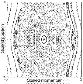
Figure 1: Poincaré section for a classical particle in an amplitude-modulated optical standing wave. Momentum and position (one well of the standing wave) of the particle along the standing wave are plotted stroboscopically with the stroboscopic period being equal to the modulation period. The central region consists of small amplitude motion. Chaos (dotted region) separates this region from two period-1 regions of regular motion (represented in the Poincaré section as sets of closed curves) located left and right of the centre along momentum $p=0$ . Further out in momentum are two stable regions of motion known as librations. At the edges are bands of regular motion corresponding to above barrier motion. It is plotted for modulation parameter $\varepsilon=0.20$ and scaled well depth $\kappa=1.20$.

Two symmetric regular regions can be observed about $(q=0,p=1)$ and $(q=0,p=-1)$. These regions correspond to oscillatory motion in phase with the amplitude modulation in each well of the standing wave. In the experiment Hensinger et al. (2001a); Hensinger et al. (2003) atoms are loaded in a period-1 region of regular motion by controlling their initial position and momentum and by choosing the starting phase of the amplitude modulation appropriately. Classically atoms should retain their momentum state when observed stroboscopically (time step is one modulation period). A distinct signature of dynamical tunnelling is a coherent oscillation of the stroboscopically observed mean momentum as shown in Fig. 2 and reported in ref. Hensinger et al. (2001a).

In Sec. II we introduce the theoretical tools to analyze dynamical tunnelling by discussing Gross-Pitaevskii simulations and the appropriate Floquet theory. We present a thorough analysis of the experiments from ref. Hensinger et al. (2001a) in Sec. III. After showing some theoretical results for the experimental parameters we give a small overview of what to expect when some of the system parameters in the experiments are varied in Sec. IV and give some initial analysis. In Sec. V we point to pathways to analyze the quantum-classical transition for our experimental system and give conclusions in Sec. VI.

II Theoretical analysis of the dynamic evolution of a Bose-Einstein condensate

II.1 Dynamics using the Gross-Pitaevskii equation

The dynamics of a Bose-Einstein condensate in a time-dependent potential in the mean-field limit are described by the Gross-Pitaevskii equation Dalfovo et al. (1999); Parkins and Walls (1997)

$$i\hbar\frac{\partial\Psi\left(\mathbf{r},t\right)}{\partial t} =\bigg{[}-\frac{\hbar}{2m}\nabla^{2}+V_{trap}\left(\mathbf{r},t\right)+V\left(\mathbf{r},t\right)$$

$$\hskip 28.45274pt+N\frac{4\pi\hbar^{2}a}{m}\left|\Psi\left(\mathbf{r},t\right)\right|^{2}\bigg{]}\Psi\left(\mathbf{r},t\right)$$ (5)

where $N$ is the mean number of atoms in the condensate, $a$ is the scattering length with $a=2.8$ nm for sodium. $V_{trap}\left(\mathbf{r}\right)$ is the trapping potential which is turned off during the interaction with the standing wave and $V\left(\mathbf{r},t\right)$ is the time dependent optical potential induced by the optical standing wave. The Gross-Pitaevskii equation is propagated in time using a standard numerical split-operator, fast Fourier transform method. The size of the spatial grid of the numerical simulation is chosen to contain the full spatial extent of the initial condensate (therefore all the populated wells of the standing wave), and the grid has periodic boundary conditions at each side (a few unpopulated wells are also included on each side).

To obtain the initial wave function a Gaussian test function is evolved by imaginary time evolution to converge to the ground state of the stationary Gross-Pitaevskii equation. Then the standing wave is turned on adiabatically with $V\left(\mathbf{r},t\right)$ approximately having the form of a linear ramp. After the adiabatic turn-on, the condensate wave function is found to be localized at the bottom of each well of the standing wave. The standing wave is shifted and the time-dependent potential now has the form

$$V\left(\mathbf{r},t\right)=\frac{\hbar\Omega_{\mathrm{eff}}}{4}\left({1-2\varepsilon\sin}\left({\omega t+\phi}\right)\right)\sin^{2}(kx+\varphi)$$ (6)

where $\varphi$ is the phase shift which is applied to selectively load one region of regular motion Hensinger et al. (2001a). The position representation of the atomic wave function $\left|\Psi\left(\mathbf{r}\right)\right|^{2}$ just before the modulation starts (and after the phase shift) is shown in Fig. 3 ($t=0T$).

The Gross-Pitaevskii equation is used to model the experimental details of a Bose-Einstein condensate in an optical 1-D lattice. The experiment effectively consists of many coherent single-atom experiments. The coherence is reflected in the occurrence of diffraction peaks in the atomic momentum distribution (see Fig. 4). Utilizing the Gross-Pitaevskii equation, the interaction between these single-atom experiments is modelled by a classical field. Although ignoring quantum phase fluctuations in the condensate, the wave nature of atoms is still contained in the Gross-Pitaevskii equation and dynamical tunnelling is a quantum effect that results from the wave nature of the atoms. The assumption for a common phase for the whole condensate is well justified for the experimental conditions as the timescales of the experiment and the lattice well depth are sufficiently small. It will be shown in the following (see Fig. 8) that the kinetic energy is typically of the order of $10^{5}$ Hz which is much larger than the non-linear term in the Gross-Pitaevskii equation 5 which is on the order of 400 Hz. The experimental results, in particular dynamical tunnelling could therefore be modelled by a single particle Schrödinger equation in a one-dimensional single well with periodic boundary conditions. Nevertheless the Gross-Pitaevskii equation is used to model all the experimental details of a Bose-Einstein condensate in an optical lattice to guarantee maximum accuracy. We will discuss and compare the Gross-Pitaevskii and the Floquet approaches below (last paragraph of section II).

Theoretical analysis of the dynamical tunnelling experiments will be presented in this paper utilizing numerical solutions of the Gross-Pitaevskii equation. Furthermore we will analyze the system parameter space which is spanned by the scaled well depth $\kappa,$ the modulation parameter $\varepsilon$ and the scaled Planck’s constant ${\mathchoice{\hbox{\lower 0.70007pt\hbox{$\mathchar 22\relax$}}}{\hbox{\lower 0.70007pt\hbox{$\mathchar 22\relax$}}}{\hbox{\lower 0.48996pt\hbox{$\scriptstyle\mathchar 22\relax$}}}{\hbox{\lower 0.35004pt\hbox{$\scriptscriptstyle\mathchar 22\relax$}}}\mkern-8.0muk}$. In fact variation of the scaled Planck’s constant in the simulations allows one to move the quantum system towards the classical limit.

II.2 Floquet analysis

The quantum dynamics of a periodically driven Hamiltonian system can be described in terms of the eigenstates of the Floquet operator $F$, which evolves the system in time by one modulation period. In the semiclassical regime, the Floquet eigenstates can be associated with regions of regular and irregular motion of the classical map. However when $\hbar$ is not sufficiently small compared to a typical classical action the phase-space representation of the Floquet eigenstates do not necessarily match with some classical (regular or irregular) structuresDyrting et al. (1993); Mouchet et al. (2001). However, initial states localized at the stable region around a fixed point in the Poincaré section can be associated with superpositions of a small number of Floquet eigenstates. Using this state basis, one can reveal the analogy of the dynamical tunnelling experiments and conventional tunnelling in a double well system. Two states of opposite parity which can be responsible for the observed dynamical tunnelling phenomenon are identified. Floquet states are stroboscopic eigenstates of the system. Their phase space representation therefore provides a quantum analogue to the classical stroboscopic phase space representation, the Poincaré map.

Only very few states are needed to describe the evolution of a wave packet that is initially strongly localized on a region of regular motion. A strongly localized wavepacket is used in the experiments (strongly localized in each well of the standing wave) making the Floquet basis very useful. In contrast, describing the dynamics in momentum or position representation requires a large number of states so that some of the intuitive understanding which one can obtain in the Floquet basis is impossible to gain. For example, the tunnelling period can be derived from the quasi-eigenenergies of the relevant Floquet states, as will be shown below.

For an appropriate choice of parameters the phase space exhibits two period-1 fixed points, which for a suitable Poincaré section lie on the momentum axis at $\pm p_{0}$, as in reference Hensinger et al. (2001a). For certain values of the scaled well depth $\kappa$ and   modulation parameter $\varepsilon$ there are two dominant Floquet states $|\phi_{\pm}\rangle$ that are localized on both fixed points but are distinguished by being even or odd eigenstates of the parity operator that changes the sign of momentum. A state localized on just one fixed point is therefore likely to have dominant support on an even or odd superposition of these two Floquet states:

$$|\psi\left(\pm p_{0}\right)\rangle\approx\left(|\phi_{+}\rangle\pm|\phi_{-}\rangle\right)/\sqrt{2}.$$ (7)

The stroboscopic evolution is described by repeated application of the Floquet operator. As this is a unitary operator,

$$F|\phi_{\pm}\rangle=e^{\left(-i2\pi\phi_{\pm}/{\mathchoice{\hbox{\lower 0.49005pt\hbox{$\mathchar 22\relax$}}}{\hbox{\lower 0.49005pt\hbox{$\mathchar 22\relax$}}}{\hbox{\lower 0.34297pt\hbox{$\scriptstyle\mathchar 22\relax$}}}{\hbox{\lower 0.24503pt\hbox{$\scriptscriptstyle\mathchar 22\relax$}}}\mkern-8.0muk}\right)}|\phi_{\pm}\rangle.$$ (8)

$\phi_{\pm}$ are the Floquet quasienergies. Thus at a time which is $n$ times the period of modulation, the state initially localized on $+p_{0}$, evolves to

$$|\psi\left(n\right)\rangle\approx\left(e^{\left(-i2\pi n\phi_{+}/{\mathchoice{\hbox{\lower 0.49005pt\hbox{$\mathchar 22\relax$}}}{\hbox{\lower 0.49005pt\hbox{$\mathchar 22\relax$}}}{\hbox{\lower 0.34297pt\hbox{$\scriptstyle\mathchar 22\relax$}}}{\hbox{\lower 0.24503pt\hbox{$\scriptscriptstyle\mathchar 22\relax$}}}\mkern-8.0muk}\right)}|\phi_{+}\rangle+e^{\left(-i2\pi n\phi_{-}/{\mathchoice{\hbox{\lower 0.49005pt\hbox{$\mathchar 22\relax$}}}{\hbox{\lower 0.49005pt\hbox{$\mathchar 22\relax$}}}{\hbox{\lower 0.34297pt\hbox{$\scriptstyle\mathchar 22\relax$}}}{\hbox{\lower 0.24503pt\hbox{$\scriptscriptstyle\mathchar 22\relax$}}}\mkern-8.0muk}\right)}|\phi_{-}\rangle\right)/\sqrt{2}.$$ (9)

Ignoring an overall phase and defining the separation between Floquet quasienergies as

$$\Delta\phi=\phi_{-}-\phi_{+},$$ (10)

one obtains

$$|\psi\left(n\right)\rangle\approx\left(|\phi_{+}\rangle+e^{\left(-i2\pi n\Delta\phi/{\mathchoice{\hbox{\lower 0.49005pt\hbox{$\mathchar 22\relax$}}}{\hbox{\lower 0.49005pt\hbox{$\mathchar 22\relax$}}}{\hbox{\lower 0.34297pt\hbox{$\scriptstyle\mathchar 22\relax$}}}{\hbox{\lower 0.24503pt\hbox{$\scriptscriptstyle\mathchar 22\relax$}}}\mkern-8.0muk}\right)}|\phi_{-}\rangle\right)/\sqrt{2}.$$ (11)

At

$$n={\mathchoice{\hbox{\lower 0.70007pt\hbox{$\mathchar 22\relax$}}}{\hbox{\lower 0.70007pt\hbox{$\mathchar 22\relax$}}}{\hbox{\lower 0.48996pt\hbox{$\scriptstyle\mathchar 22\relax$}}}{\hbox{\lower 0.35004pt\hbox{$\scriptscriptstyle\mathchar 22\relax$}}}\mkern-8.0muk}/2\Delta\phi$$ (12)

periods, the state will form the anti-symmetric superposition of Floquet states and thus is localized on the other fixed point at $-p_{0}$. In other words the atoms have tunnelled from one of the fixed points to the other. This is reminiscent of barrier tunnelling between two wells, where a particle in one well, in a superposition of symmetric and antisymmetric energy eigenstates, oscillates between wells with a frequency given by the energy difference between the eigenstates.

Tunnelling can also occur when the initial state has significant overlap with two non-symmetric states. For example, if the initial state is localized on two Floquet states, one localized inside the classical chaotic region and one inside the region of regular motion, a distinct oscillation in the stroboscopic evolution of the mean momentum may be visible. The frequency of this tunnelling oscillation depends on the spacing of the corresponding quasi-eigenenergies in the Floquet spectrum. In many cases multiple tunnelling frequencies occur in the stroboscopic evolution of the mean momentum some of which are due to tunnelling between non-symmetric states.

Quantum dynamical tunnelling may be defined in that a particle can access a region of phase space in a way that is forbidden by the classical dynamics. This implies that it crosses a Kolmogorov-Arnold-Moser (KAM) surface Berry (1978); Arnold (1979). The clearest evidence of dynamical tunnelling can be obtained by choosing the scaled Planck’s constant ${\mathchoice{\hbox{\lower 0.70007pt\hbox{$\mathchar 22\relax$}}}{\hbox{\lower 0.70007pt\hbox{$\mathchar 22\relax$}}}{\hbox{\lower 0.48996pt\hbox{$\scriptstyle\mathchar 22\relax$}}}{\hbox{\lower 0.35004pt\hbox{$\scriptscriptstyle\mathchar 22\relax$}}}\mkern-8.0muk}$ sufficiently small so that the atomic wavefunction is much smaller than the region of regular motion (the size of the wave function is given by ${\mathchoice{\hbox{\lower 0.70007pt\hbox{$\mathchar 22\relax$}}}{\hbox{\lower 0.70007pt\hbox{$\mathchar 22\relax$}}}{\hbox{\lower 0.48996pt\hbox{$\scriptstyle\mathchar 22\relax$}}}{\hbox{\lower 0.35004pt\hbox{$\scriptscriptstyle\mathchar 22\relax$}}}\mkern-8.0muk}$). Furthermore it should be centered inside the region of regular motion. However, even if the wave packet is larger than the region of regular motion and also populates the classical chaotic region of phase space one can still analyze quantum-classical correspondence and tunnelling. One assumes a classical probability distribution of point particles with the same size as the quantum wave function and compares the classical evolution of this point particle probability distribution with the quantum evolution of the wave packet. A distinct difference between the two evolutions results from the occurrence of tunnelling assuming that the quantum evolution penetrates a KAM surface visibly.

II.3 Comparison

Using the Gross-Pitaevskii equation one can exactly simulate the experiment because the momentum or position representation is used. Therefore the theoretical simulation can be directly compared with the experimental result. In contrast Floquet states do not have a straightforward experimental intuitive analogue. In the Floquet states analysis one can compare the quasienergy splitting between the tunnelling Floquet state with the experimentally measured tunnelling period. The occurrence of multiple frequencies in the experimentally observed tunnelling oscillations might also be explained with the presence of more than two dominant Floquet states, the tunnelling frequencies being the energy splitting between different participating Floquet states. Using the Gross-Pitaevskii approach one can simulate the experiment with high precision. The same number of populated wells as in the experiment can be used and the turn-on of the standing wave can be simulated using an appropriate turn-on Hamiltonian. Therefore one can obtain the correct initial state with high precision. Furthermore the mean-field interaction is simulated which is not contained in the Floquet approach.

III Numerical simulations of the experiments

III.1 Gross-Pitaevskii simulations

In this section experimental results that were discussed in a previous paper Hensinger et al. (2001a) are compared with numerical simulations of the Gross-Pitaevskii (GP) equation.

In the experiment Hensinger et al. (2001a) the atomic wave function was prepared initially to be localized around a period-1 region of regular motion. Figure 2 shows the stroboscopically measured mean momentum as a function of the interaction time with the standing wave for modulation parameter $\varepsilon=0.29$, scaled well depth $\kappa=1.66$, modulation frequency $\omega/2\pi=250$ kHz and a phase shift of $\varphi=0.21\cdot 2\pi.$

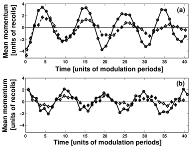
Figure 2: Stroboscopic mean momentum as a function of the interaction time with the modulated standing wave measured in modulation periods, $n$, for modulation parameter $\varepsilon=0.29$, scaled well depth $\kappa=1.66$, modulation frequency $\omega/2\pi=250$ kHz and a phase shift $\varphi=0.21\cdot 2\pi.$ (a) and (b) correspond to the two different interaction times $n+0.25$ and $n+0.75$ modulation periods, respectively. Results from the dynamic evolution of the Gross-Pitaevskii equation are plotted as solid line (circles) and the experimental data are plotted as dashed line (diamonds).

(a) and (b) correspond to the two different interaction times $n+0.25$ (standing wave modulation ends at a maximum of the amplitude modulation) and $n+0.75$ modulation periods (standing wave modulation ends at a minimum of the amplitude modulation), respectively. Results from the simulations (solid line, circles) are compared with the experimental data (dashed line, diamonds). Dynamical tunnelling manifests itself as a coherent oscillation of the stroboscopically observed mean momentum. This occurs in contrast to the classical prediction in which atoms should retain their momentum state when observed stroboscopically (time step is one modulation period). There is good agreement between experiment and theory as far as the tunnelling period is concerned. However, the experimentally measured tunnelling amplitude is smaller than the theoretical prediction.

It should be noted that the theoretical simulations do not take account of any possible spatial and temporal variations of the scaled well depth (eg. light intensity), which could possibly lead to the observed discrepancy. It was decided to produce simulations without using any free parameters. However the uncertainty associated with the experiment would allow small variations of the modulation parameter $\varepsilon$ and the scaled well depth $\kappa.$ There was a 10% uncertainty in the value of the scaled well depth $\kappa$ and a 5% uncertainty in the modulation parameter $\varepsilon$ (all reported uncertainties are 1 s.d. combined systematic and statistical uncertainties). Both temporal and spatial uncertainty during one run of the experiment are contained in these values as well as the systematic total measurement uncertainty. It was verified that there are no important qualitative changes when varying the parameters in the uncertainty regime for the simulations presented here. However, the agreement between experiment and theory often can be optimized (not always non-ambiguously, meaning that it is sometimes hard to decide which set of parameters produces the best fit). Although the theoretical simulation presented does not show any decay in the mean momentum curve, a slight change of parameters inside the experimental uncertainty can lead to decay which is most likely caused by another dominant Floquet state whose presence leads to the occurrence of a beating of the tunnelling oscillations which appears as decay (and revival on longer time scales). A detailed analysis of the corresponding Floquet states and their meaning will be presented in Sec. III.3. An example of how a change of parameters inside the experimental uncertainty in the simulations can optimize the agreement between theory and experiment is shown in Fig. 6 and Fig. 7. Both figures are described in more detail later in this section. Another reason for the observed discrepancy could be the evolution of non-condensed atoms that is not contained in the GP approach and the interaction of non-condensed atoms with the condensate. With a sufficiently long adiabatic turn-on time of the far detuned standing wave the production of non-condensed atoms should be negligible. The interaction of the condensate with non-condensed atoms should also be negligible due to the low atomic density (note that in the experiments the condensate is expanded before the standing wave is turned on). However, further studies are needed to give an exact estimate of these effects.

The position representation of the atomic wave function $\left|\Psi\left(x\right)\right|^{2}$ is plotted stroboscopically after multiples of one modulation period in Fig. 3 for the same parameters as Fig. 2.

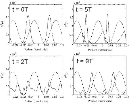
Figure 3: Position representation of the atomic wave function as a function of the number of modulation periods calculated using the Gross-Pitaevskii equation. The wave packet is plotted stroboscopically at a phase so it is located classically approximately at its highest point in the potential well. The position of the standing wave wells is also shown (dotted line). Dynamical tunnelling can be observed. At $t=5T$ most atoms have tunnelled into the other period-1 region of regular motion. The position axis is given in Fermi units (scaled by the mean Thomas-Fermi diameter).

The position of the standing wave wells is also shown (dotted line), their amplitude is given in arbitrary units. The position axis is scaled with the mean Thomas-Fermi diameter. The initial modulation phase is chosen so that the wavepacket should be located classically approximately at its highest point of the potential well Hensinger et al. (2003). Choosing this stroboscopic phase the two regions of regular motion are always maximally separated in position space. Using this phase for the stroboscopic plots enables the observation of dynamical tunnelling in position space as the two regions of regular motion are located to the left and to the right of the minimum of the potential well, being maximally spatially separated. In contrast, in the experiments, tunnelling is always observed in momentum space (the standing wave is turned off when the regions of regular motion are at the bottom of the well, overlapping spatially but having oppositely directed momenta) as it is difficult to optically resolve individual wells of the standing wave. The first picture in Fig. 3 ($t=0T$) shows the initial wave packet before the modulation is turned on. Subsequent pictures exemplify the dynamical tunnelling process. At $t=2T,$ half the atoms have tunnelled; most of the atoms are in the other region of regular motion at $t=5T$. The atoms have returned to their initial position at about $t=9T$. The double peak structure at $t=5T$ and the small central peak at $t=2T$ could indicate that Floquet states other than the two dominant ones are also loaded which is likely as a relatively large Planck’s constant was used enabling the initial wave packet to cover a substantial phase space area.

Figure 4 shows simulations of the stroboscopically measured momentum distributions $\left|\Psi\left(p\right)\right|^{2}$ as bar graphs for the same parameters as Fig. 3.

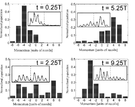
Figure 4: Momentum distributions as a function of the interaction time with the modulated standing wave calculated using numerical solutions of the Gross-Pitaevskii equation for the same parameters as Fig. 3. Initially atoms have mostly negative momentum ($t=0.25T$). After approximately 5 modulation periods most atoms populate a state with positive momentum, therefore having undergone dynamical tunnelling. Corresponding experimental data from reference Hensinger et al. (2001a) is also included as insets.

Corresponding experimental data from reference Hensinger et al. (2001a) are also included as insets. The momentum distributions are plotted at $n+0.25$ modulation periods, where $n$ is an integer. At this modulation phase the amplitude modulation is at its maximum and atoms in a period-1 region of regular motion are classically at the bottom of the well having maximum momentum. The two period-1 regions of regular motion can be distinguished in their momentum representation at this phase as they have opposite momenta. At $t=0.25T$ the atoms which were located initially half way up the potential well as shown in Fig. 3 at $t=0T$ have “rolled” down the well having acquired negative momentum. Momentum distributions for subsequent times illustrate the dynamical tunnelling process. At $t=5.25$ modulation periods most atoms have reversed their momentum and they return to their initial momentum state at approximately $t=9.25T$. The simulations are in reasonable agreement with the experimentally measured data.

Dynamical tunnelling is sensitive to the modulation parameter, the scaled well depth and the scaled Planck’s constant. To illustrate this, tunnelling data along with the appropriate evolution of the Gross Pitaevskii equation will be shown for another two parameter sets. Even though this represents only a small overview of the parameter dependency of the tunnelling oscillations it may help to appreciate the variety of features in the atomic dynamics. Figure 5 shows the theoretical simulation and the experimental data for $\varepsilon=0.28$, $\kappa=1.49$, $\omega/2\pi=250$ kHz, and $\varphi=0.22\cdot 2\pi.$ The mean momentum is plotted stroboscopically with the intensity modulation at maximum ($n+0.25$ modulation periods, $n$ being an integer). The solid line (circles) is produced by a Gross-Pitaevskii simulation and the dashed line (diamonds) consists of experimental data.

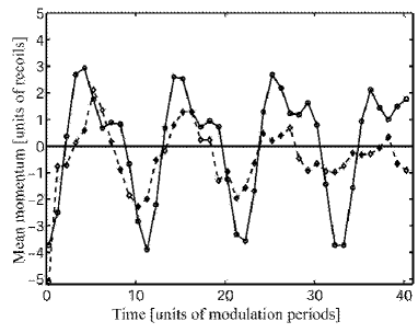
Figure 5: Mean momentum as a function of the interaction time with the modulated standing wave measured in modulation periods, $n,$ for $\varepsilon=0.28$, $\kappa=1.49$, $\omega/2\pi=250$ kHz, and $\varphi=0.22\cdot 2\pi.$ The points are plotted stroboscopically with an interaction time of $n+0.25$ modulation periods which corresponds to turning off the standing wave at maximum. Results from the dynamic evolution of the Gross-Pitaevskii equation are plotted as solid line (circles) and the experimental data is plotted as dashed line (diamonds).

There are approximately 3.5 tunnelling periods in 40 modulation periods in the theoretical curve.

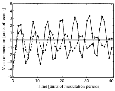
Figure 6: Mean momentum as a function of the interaction time with the modulated standing wave measured in modulation periods, $n$, for modulation parameter $\varepsilon=0.30$, scaled well depth $\kappa=1.82$, modulation frequency $\omega/2\pi=222$ kHz and phase shift $\varphi=0.21\cdot 2\pi$. The points are plotted stroboscopically with an interaction time of $n+0.25$ modulation periods which corresponds to turning off the standing wave at maximum. Results from the dynamic evolution of the Gross-Pitaevskii equation are plotted as solid line (circles) and the experimental data is plotted as dashed line (diamonds).

Figure 6 shows the mean momentum as a function of the interaction time with the standing wave for modulation parameter $\varepsilon=0.30$, scaled well depth $\kappa=1.82$, modulation frequency $\omega/2\pi=222$ kHz and phase shift $\varphi=0.21\cdot 2\pi$. For these parameters the tunnelling frequency is larger than for the parameters shown in Fig. 5.

The simulation shows good agreement with the experiment. However, the theoretical mean momentum tunnelling amplitude is larger than the one measured in the experiment and the theoretical tunnelling frequency for this set of parameters is slightly larger than the experimentally measured one.

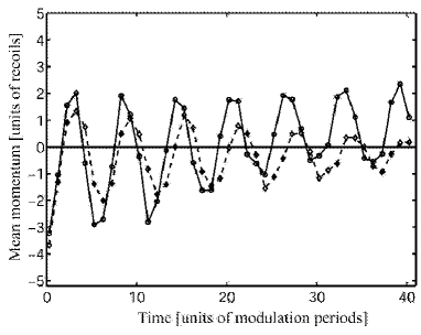
Figure 7: Mean momentum as a function of the interaction time with the modulated standing wave measured in modulation periods, $n$, using the same parameters as Fig. 6 but the modulation parameter $\varepsilon$ is reduced from 0.30 to 0.28 for the theoretical simulation. A much better fit is obtained.

Figure 7 illustrates that one can achieve much better agreement between experiment and simulation if one of the parameters is varied inside the experimental regime of uncertainty. The theoretical curve in this figure is obtained using the same parameters as in Fig. 6, but the modulation parameter $\varepsilon$ is reduced from 0.30 to 0.28. The tunnelling amplitude and frequency is now very similar to the experimental results. Note that the experimental data is not centered at zero momentum. This is also the case in the theoretical simulations for both $\varepsilon=0.28$ and $\varepsilon=0.30$. The mean momentum curve appears much more sinusoidal than the one for $\varepsilon=0.29$, $\kappa=1.66$, $\omega/2\pi=250$ kHz and $\varphi=0.21\cdot 2\pi$ (Fig. 2). This could imply that the initial wave function has support on fewer Floquet states.

III.2 Stroboscopic evolution of the system energies

Calculating the expectation values of the relevant system energies can give important information about the relevant energy scales and it might also help to obtain a deeper insight into the stroboscopic evolution of a Bose-Einstein condensate in a periodically modulated potential. Figure 8 shows the energy expectation values for the mean-field energy, the potential energy and the kinetic energy given in Hz (scaled by Planck’s constant).

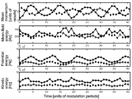
Figure 8: Stroboscopic evolution of mean-field energy, the kinetic energy and the potential energy. The energies are given in Hz (energy is scaled with Planck’s constant). For comparison the mean momentum is also shown as a function of the interaction time with the standing wave (in units of modulation periods). The solid (circles) and dashed (diamonds) curves correspond to the two different interaction times $n+0.25$ and $n+0.75$ modulation periods, respectively. The evolution is plotted for modulation parameter $\varepsilon=0.29$, scaled well depth $\kappa=1.66$, modulation frequency $\omega/2\pi=250$ kHz and a phase shift $\varphi=0.21\cdot 2\pi$.

For comparison the stroboscopic mean momentum expectation values are also shown. The energy and momentum expectation values are plotted stroboscopically and the solid (circles) and dashed (diamonds) curves correspond to the two different interaction times $n+0.25$ and $n+0.75$ modulation periods, respectively. Figure 8 is plotted for modulation parameter $\varepsilon=0.29$, scaled well depth $\kappa=1.66$, modulation frequency $\omega/2\pi=250$ kHz and a phase shift of $\varphi=0.21\cdot 2\pi$ which corresponds to Fig. 2. The mean-field energy is three orders of magnitude smaller than the potential or the kinetic energy. While the kinetic energy does not show a distinct oscillation, an oscillation is clearly visible in the stroboscopic potential energy evolution. This oscillation frequency is not equal to the tunnelling frequency but it is smaller as can be seen in Fig. 8. One obtains a period of approximately 8.9 modulation periods compared to a tunnelling period of approximately 10.0 modulation periods. Considering the energy scales one should note that this oscillation is also clearly visible in the stroboscopic evolution of the total energy of the atoms. The origin of this oscillation is not known yet and will be the subject of future investigation.

III.3 Floquet analysis for some experimental parameters

Time and spatial periodicity of the Hamiltonian allow utilization of the Bloch and Floquet theorems Mouchet et al. (2001); Ashcroft and Mermin (1976). Because of the time periodicity, there still exists eigenstates of the evolution operator over one period (Floquet theorem). Its eigenvalues can be written in the form $e^{-i2\pi\phi_{n}\tau/{\mathchoice{\hbox{\lower 0.49005pt\hbox{$\mathchar 22\relax$}}}{\hbox{\lower 0.49005pt\hbox{$\mathchar 22\relax$}}}{\hbox{\lower 0.34297pt\hbox{$\scriptstyle\mathchar 22\relax$}}}{\hbox{\lower 0.24503pt\hbox{$\scriptscriptstyle\mathchar 22\relax$}}}\mkern-8.0muk}}$ where $\phi_{n}$ is called the quasienergy of the states. $n$ is a discrete quantum number. Due to the spatial $\lambda/2$-periodicity, in addition to $n$, these states are labeled by a continuous quantum number, the so called quasi-momentum $\vartheta\in\left[-2\pi/\lambda,2\pi/\lambda\right[$ (Bloch theorem). The quasienergy spectrum $\phi_{n}(\vartheta)$ is therefore made of bands labelled by $n$ (see for instance Fig. 10). More precisely, the states can be written as

$$\left|\phi_{n,\vartheta}\left(\tau\right)\right\rangle=e^{\left(-i2\pi\phi_{n}\left(\vartheta\right)\tau/{\mathchoice{\hbox{\lower 0.49005pt\hbox{$\mathchar 22\relax$}}}{\hbox{\lower 0.49005pt\hbox{$\mathchar 22\relax$}}}{\hbox{\lower 0.34297pt\hbox{$\scriptstyle\mathchar 22\relax$}}}{\hbox{\lower 0.24503pt\hbox{$\scriptscriptstyle\mathchar 22\relax$}}}\mkern-8.0muk}\right)}e^{\left(-i\vartheta q\right)}\left|\psi_{n,\vartheta}\left(\tau\right)\right\rangle$$ (13)

where $\left\{\left|\psi_{n,\vartheta}\left(\tau\right)\right\rangle\right\}$ is now strictly periodic in space and time (i.e. not up to a phase).

The evolution of the initial atomic wave function can be easily computed from its expansion on the $\left|\phi_{n,\vartheta}\left(0\right)\right\rangle$ once the Floquet operator has been diagonalized. The $\left|\psi_{n,\vartheta}\left(\tau\right)\right\rangle$ are the eigenstates of the modified Floquet-Bloch Hamiltonian

$$\mathcal{H}=\left(p+{\mathchoice{\hbox{\lower 0.70007pt\hbox{$\mathchar 22\relax$}}}{\hbox{\lower 0.70007pt\hbox{$\mathchar 22\relax$}}}{\hbox{\lower 0.48996pt\hbox{$\scriptstyle\mathchar 22\relax$}}}{\hbox{\lower 0.35004pt\hbox{$\scriptscriptstyle\mathchar 22\relax$}}}\mkern-8.0muk}\vartheta\right)^{2}/2+2\kappa(1-2\varepsilon\sin\tau)\sin^{2}(q/2)$$ (14)

subjected to strictly periodic space-time boundary conditions.

Dominant Floquet states may be determined by calculating the inner product of the Floquet states with the initial atomic wavefunction. To obtain a phase space representation of Floquet states in momentum and position space one can calculate the Husimi or Q-function. It is defined as

$$Q\left(q,p,\tau\right)=\frac{1}{2\pi{\mathchoice{\hbox{\lower 0.70007pt\hbox{$\mathchar 22\relax$}}}{\hbox{\lower 0.70007pt\hbox{$\mathchar 22\relax$}}}{\hbox{\lower 0.48996pt\hbox{$\scriptstyle\mathchar 22\relax$}}}{\hbox{\lower 0.35004pt\hbox{$\scriptscriptstyle\mathchar 22\relax$}}}\mkern-8.0muk}}\left|\left\langle q+ip|\phi\right\rangle\right|^{2}$$ (15)

where $|q+ip\rangle$ is the coherent state of a simple harmonic oscillator with frequency $\omega_{0}$ chosen as $\sqrt{\kappa}$ in scaled units. The position representation $\left\langle q^{\prime}|q+ip\right\rangle$ of the coherent state Klauder and Skagerstam (1985); Cohen-Tannoudji et al. (1977) is given by

$$\left\langle q^{\prime}|q+ip\right\rangle=\left(\frac{\omega_{0}}{\pi{\mathchoice{\hbox{\lower 0.70007pt\hbox{$\mathchar 22\relax$}}}{\hbox{\lower 0.70007pt\hbox{$\mathchar 22\relax$}}}{\hbox{\lower 0.48996pt\hbox{$\scriptstyle\mathchar 22\relax$}}}{\hbox{\lower 0.35004pt\hbox{$\scriptscriptstyle\mathchar 22\relax$}}}\mkern-8.0muk}}\right)^{1/4}\exp\left\{-\left[\frac{q^{\prime}-q}{2\Delta}\right]^{2}+ip\frac{q}{{\mathchoice{\hbox{\lower 0.70007pt\hbox{$\mathchar 22\relax$}}}{\hbox{\lower 0.70007pt\hbox{$\mathchar 22\relax$}}}{\hbox{\lower 0.48996pt\hbox{$\scriptstyle\mathchar 22\relax$}}}{\hbox{\lower 0.35004pt\hbox{$\scriptscriptstyle\mathchar 22\relax$}}}\mkern-8.0muk}}\right\}$$ (16)

up to an overall phase factor and where $\Delta=\sqrt{\frac{{\mathchoice{\hbox{\lower 0.49005pt\hbox{$\mathchar 22\relax$}}}{\hbox{\lower 0.49005pt\hbox{$\mathchar 22\relax$}}}{\hbox{\lower 0.34297pt\hbox{$\scriptstyle\mathchar 22\relax$}}}{\hbox{\lower 0.24503pt\hbox{$\scriptscriptstyle\mathchar 22\relax$}}}\mkern-8.0muk}}{2\omega_{0}}}$. Floquet analysis will be shown for some of the experimental parameters which were presented in the previous section.

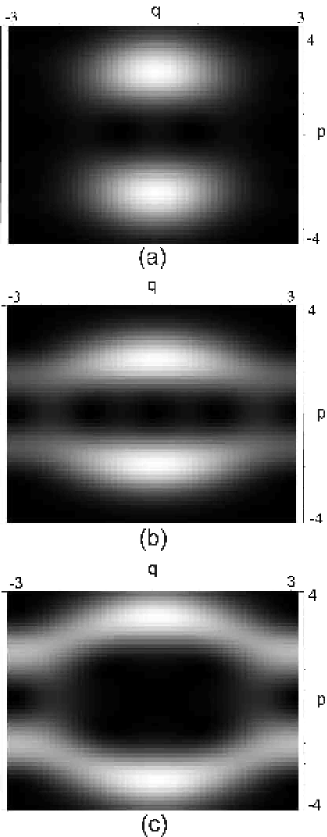
Figure 9: Phase space representations of two Floquet states for $\vartheta=0$ that are involved in the dynamical tunnelling are shown in (a) and (b). The Floquet states correspond to the experimental parameters: modulation parameter $\varepsilon=0.29$, scaled well depth $\kappa=1.66$ and modulation frequency $\omega/2\pi=250$ kHz, which were utilized to obtain the experimental results shown in Fig. 2. A third state, shown in (c) also has significant overlap with the initial experimental state.

Figure 9 shows contour plots of the Husimi functions of two Floquet states with opposite parity ((a), (b)) for these parameters whose presence allows dynamical tunnelling to occur. Both of them are approximately localized on the classical period-1 regions of regular motion and they were selected so that the initial atomic wave function has significant overlap with them (26% and 44%, respectively). The initial experimental state has also significant overlap (22%) with a third state that is shown in Fig. 9(c). The overlap is calculated using a coherent state that is centered on the periodic region of regular motion, which is a good approximation of the initial experimental state. The quasi-eigenenergy spectrum for this set of parameters is shown in Fig. 10.

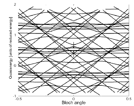
Figure 10: Quasi-eigenenergy spectrum for parameters modulation parameter $\varepsilon=0.29$, scaled well depth $\kappa=1.66$ and modulation frequency $\omega/2\pi=250$ kHz. The quasi-eigenenergy is measured in reduced energy units and it is a function of the Bloch angle. The Bloch angle is equal to the quasi-momentum multiplied with the spatial period $\lambda/2$ of the lattice. Each line corresponds to one Floquet state labelled by $n$ (see Eq.13). The quasi-eigenenergy of most Floquet states is strongly dependent on the quasi-momentum but it is not the case for the states of the tunnelling doublet. Recall that the quasi-momentum $\vartheta$ is proportional to the phase taken by a state when spatially translated by $\lambda/2$. In other words, fixing $\vartheta$ imposes on the states some conditions on the boundary of one elementary cell $[q,q+\lambda/2]$. If a state is localized deep inside a cell, changing the boundary conditions (i.e. $\vartheta$) will not affect the state so much and the corresponding quasienergies appear as curves that are approximately parallel to the $\vartheta$ axis. However, one should expect a strong $\vartheta$-dependence for a state that spread over at least $\Delta q\sim\lambda/2$.

The quasi-eigenenergies are plotted as a function of the quasi-momentum (Bloch angle). Each line corresponds to one Floquet state labelled by $n$ (see Eq.13). The arrows point to the two Floquet states shown in Fig. 9(a) and (b) that correspond to the tunnelling splitting in Eq.  10. Most of the other lines correspond to Floquet states which lie in the classical chaotic phase space region. Examples of phase space representations of such Floquet states can be found in reference Mouchet et al. (2001). Note that the spectrum is $2\pi{\mathchoice{\hbox{\lower 0.70007pt\hbox{$\mathchar 22\relax$}}}{\hbox{\lower 0.70007pt\hbox{$\mathchar 22\relax$}}}{\hbox{\lower 0.48996pt\hbox{$\scriptstyle\mathchar 22\relax$}}}{\hbox{\lower 0.35004pt\hbox{$\scriptscriptstyle\mathchar 22\relax$}}}\mkern-8.0muk}/T$ periodic in quasienergies. For quasi-momentum $\vartheta=0$ the splitting between the two states, that are shown in Fig. 9 is approximately 0.08 in reduced units (energy in frequency units, [energy$/\left(2\pi{\mathchoice{\hbox{\lower 0.70007pt\hbox{$\mathchar 22\relax$}}}{\hbox{\lower 0.70007pt\hbox{$\mathchar 22\relax$}}}{\hbox{\lower 0.48996pt\hbox{$\scriptstyle\mathchar 22\relax$}}}{\hbox{\lower 0.35004pt\hbox{$\scriptscriptstyle\mathchar 22\relax$}}}\mkern-8.0muk}\right)$]). With a modulation frequency $\omega/2\pi=250$ kHz one obtains a scaled Planck’s constant ${\mathchoice{\hbox{\lower 0.70007pt\hbox{$\mathchar 22\relax$}}}{\hbox{\lower 0.70007pt\hbox{$\mathchar 22\relax$}}}{\hbox{\lower 0.48996pt\hbox{$\scriptstyle\mathchar 22\relax$}}}{\hbox{\lower 0.35004pt\hbox{$\scriptscriptstyle\mathchar 22\relax$}}}\mkern-8.0muk}=0.8$, therefore the tunnelling period $T_{tun}$ which follows from Eq. 12 is 10 which is in good agreement with the experiment.

The quasi-momentum plays a significant role in the experiments. The quasi-momentum $\vartheta$ is approximately equal to the relative velocity $v$ between the wave packet (before the lattice is turned on) and the lattice, $v=\vartheta/m$ Denschlag et al. (2002) if the standing wave is adiabatically turned on. It was found in Mouchet et al. (2001) that it is of importance to populate a state whose quasi-momentum average is equal to zero. Moreover, quasi-momentum spread is also of importance. It has been shown in Mouchet and Delande (2003) that if the thermal velocity distribution is too broad, then the tunnelling oscillation disappears. As can be seen in Fig. 10 the quasi-eigenenergies of the two contributing Floquet states depend on the quasi-momentum (or Bloch angle). The tunnelling period (which is inversely proportional to the separation between these two quasi-eigenenergies) depends on the quasi-momentum. Using a thermal atomic cloud one obtains a statistical ensemble of many quasi-momenta as they initially move in random directions with respect to the optical lattice. Atoms localized in individual wells can be described by a wave packet in the plane wave basis and therefore they are characterized by a superposition of many quasi-momenta. The resulting quasi-momentum width washes out the tunnelling oscillations (see (Mouchet and Delande, 2003, Fig. 3)). In fact in another experiment Steck et al. Steck et al. (2001) found that the amplitude of the mean momentum oscillations resulting from a tunnelling process between two librational islands of stability decreased when the initial momentum width of the atomic cloud was increased.

Figure 11: Phase space representations of two Floquet states whose presence can lead to the occurrence of dynamical tunnelling. The Floquet states correspond to the experimental parameters: modulation parameter $\varepsilon=0.30$, scaled well depth $\kappa=1.82$ and modulation frequency $\omega/2\pi=222$ kHz, which were utilized to obtain the experimental results shown in Fig. 6.

Figure 11 shows contour plots of Husimi functions for the two dominant Floquet states for the modulation parameter $\varepsilon=0.30$, scaled well depth $\kappa=1.82$ and modulation frequency $\omega/2\pi=222$ kHz, which corresponds to experimental results shown in Fig. 6. The states are selected to have maximum overlap with the initial wave packet (38% and 44%). In contrast to the experimental results shown in Fig. 2 there are only two dominant Floquet states. The quasi-eigenenergy spectrum for this set of parameters (not shown) reveals a level splitting of approximately 0.15 in reduced units, the calculated tunnelling period is 6 modulation periods which is in good agreement with the experiment.

When comparing the stroboscopic evolution of the mean momentum shown in Fig. 2  (modulation parameter $\varepsilon=0.29$, scaled well depth $\kappa=1.66$ and modulation frequency $\omega/2\pi=250$ kHz) with the one shown in Fig. 6 (modulation parameter $\varepsilon=0.30$, scaled well depth $\kappa=1.82$ and modulation frequency $\omega/2\pi=222$ kHz), one finds that it is less sinusoidal. This can be explained in the Floquet picture. While there are three dominant Floquet states for the first case (Figs. 2, 9) (three Floquet states with significant overlap with the initial experimental state), there are only two dominant Floquet states for the second case (Figs. 6, 11) resulting in a more sinusoidal tunnelling oscillation.

III.4 Loading analysis of the Floquet superposition state

The initial atomic wave packet is localized around the classical period-1 region of regular motion by inducing a sudden phase shift to the standing wave. This enables the observation of dynamical tunnelling. In the Floquet picture the observation of dynamical tunnelling requires that the initial state has support on only a few dominant Floquet states, preferably populating only two with a phase space structure as shown in Fig. 9. Optimizing the overlap of the initial state with these Floquet “tunnelling” states should maximize the observed tunnelling amplitude. Here we carry out analysis confirming this prediction. This corresponds to optimizing the overlap of the initial experimental state with the period-1 regions of regular motion. Figure 12 shows the mean atomic momentum as a function of the interaction time with the standing wave which is plotted for a range of the initial phase shift $\varphi$ of the standing wave.

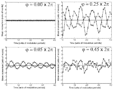
Figure 12: Mean atomic momentum as a function of the interaction time with the standing wave plotted for a range of the initial phase shift $\varphi$ of the standing wave. The solid line (circles) corresponds to an interaction time with the standing wave of $n+0.25$ modulation periods and the dashed line (diamonds) corresponds to an interaction time of $n+0.75$ modulation periods.

The solid line (circles) corresponds to an interaction time with the standing wave of $n+0.25$ modulation periods and the dashed line (diamonds) corresponds to an interaction time of $n+0.75$ modulation periods. The simulations are made using the Gross-Pitaevskii equation for modulation parameter $\varepsilon=0.29$, scaled well depth $\kappa=1.66$, modulation frequency $\omega/2\pi=250$ kHz which corresponds to Fig. 2. A phase shift $\varphi=0$ corresponds to localizing the wave packet exactly at the bottom of the well and $\varphi=\pi$ corresponds to localizing it exactly at the maximum of the standing wave well. Symmetry dictates that no tunnelling oscillation can occur for these two loading phases. This is also shown in Fig. 12 (the mean momentum curve for $\varphi=\pi$ is not shown but it is the same as for $\varphi=0$). The amplitude of the tunnelling oscillations changes strongly when the initial phase shift $\varphi$ of the standing wave is changed. The best overlap with the tunnelling Floquet states is obtained for the phase shift $\varphi$ somewhere in between $0.25\times 2\pi$ and $0.30\times 2\pi$ which corresponds to placing the wave packet half way up the standing wave well. This result is in good agreement with the structure of the tunnelling Floquet states as shown in Fig. 9. When changing $\varphi$ there is no change in the observed tunnelling period. This is to be expected as mainly the loading efficiency for the “tunnelling” Floquet states varies when $\varphi$ is varied. It should be noted that the simulations are carried out for a relatively large scaled Planck’s constant (${\mathchoice{\hbox{\lower 0.70007pt\hbox{$\mathchar 22\relax$}}}{\hbox{\lower 0.70007pt\hbox{$\mathchar 22\relax$}}}{\hbox{\lower 0.48996pt\hbox{$\scriptstyle\mathchar 22\relax$}}}{\hbox{\lower 0.35004pt\hbox{$\scriptscriptstyle\mathchar 22\relax$}}}\mkern-8.0muk}=0.8$) which means that the wave packet size is rather large compared to characteristic classical phase space features like the period-1 regions of regular motion. This analysis shows that the tunnelling amplitude sensitively depends on the loading efficiency of the tunnelling Floquet states and that there is a smooth dependency of the tunnelling amplitude on this loading parameter.

IV Parameter dependency of the tunnelling oscillations

The scaled parameter space for the dynamics of the system is given by the scaled well depth $\kappa$ and the modulation parameter $\varepsilon.$ Both parameters will significantly change the structure and number of the contributing Floquet states. It has been found that a strong sensitivity of the tunnelling frequency on the system parameters is a signature of chaos-assisted tunnelling Mouchet et al. (2001); Mouchet and Delande (2003) where a third state associated with the classical chaotic region interacts with the tunnelling Floquet states. A Floquet state that is localized inside a region of regular motion that surrounds another resonance can also interact with the tunnelling doublet (two tunnelling Floquet states), this phenomenon is known as resonance-assisted tunnelling Brodier et al. (2001).

Comprehensively exploring the parameter space and its associated phenomena is out of the scope of this article. Instead an analysis associated with our experiments will be presented here showing one scan of the scaled well depth $\kappa$ and another scan of of the modulation parameter $\varepsilon$ around the experimental parameter regime. The results are shown in the form of plots of the mean momentum as a function of the interaction time with the modulated standing wave. The solid line (circles) corresponds to an interaction time with the standing wave of $n+0.25$ modulation periods and the dashed line (diamonds) corresponds to an interaction time of $n+0.75$ modulation periods.

Figure 13 shows the scaled well depth $\kappa$ being varied from 1.10 to 1.75.

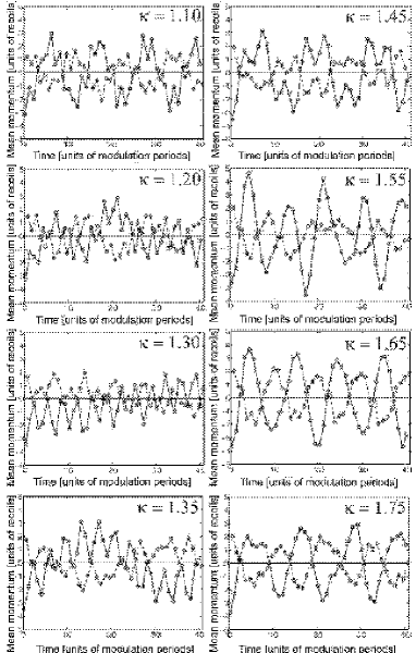
Figure 13: Mean momentum as a function of the interaction time with the modulated standing wave for different values of the scaled well depth $\kappa$ (modulation parameter $\varepsilon=0.29$, modulation frequency $\omega/2\pi=250$ kHz and phase shift $\varphi=0.21\cdot 2\pi$). The solid line (circles) corresponds to an interaction time with the standing wave of $n+0.25$ modulation periods and the dashed line (diamonds) corresponds to an interaction time of $n+0.75$ modulation periods.

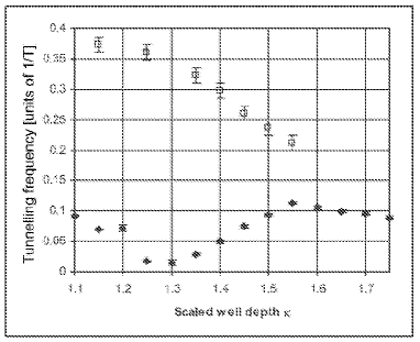
Figure 14: Tunnelling frequency as a function of the scaled well depth $\kappa$ (modulation parameter $\varepsilon=0.29$, modulation frequency $\omega/2\pi=250$ kHz and phase shift $\varphi=0.21\cdot 2\pi$) taken from Fig. 13. Diamonds and squares denote low and high frequency components, respectively.

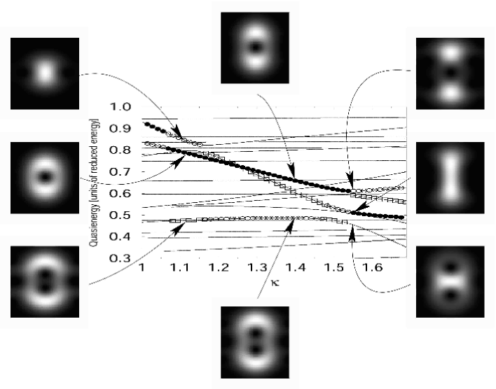
Figure 15: Floquet spectrum as a function of the scaled well depth $\kappa$ (modulation parameter $\varepsilon=0.29$, modulation frequency $\omega/2\pi=250$ kHz and phase shift $\varphi=0.21\cdot 2\pi$. The Floquet states with maximum overlap are marked black bullets, white bullets are used for second most overlap and white squared bullets show third most overlap. Phase space representations (Husimi functions) of some of the these Floquet states for different values of $\kappa$ are also shown.

The other parameters are held constant (modulation parameter $\varepsilon=0.29$, modulation frequency $\omega/2\pi=250$ kHz and phase shift $\varphi=0.21\cdot 2\pi$). The momentum distribution evolution is shown to illustrate intricate changes in the tunnelling dynamics when the parameters are varied. Both the tunnelling frequency spectrum and the tunnelling amplitude are strongly dependent on $\kappa.$ Often one can see more than just one dominant tunnelling frequency. For example, for $\kappa=1.35$ the two dominant tunnelling frequencies which contribute to the tunnelling oscillation have a period of approximately 3.9 modulation periods and approximately 34 modulation periods. In the interval of approximately $\kappa=1.5$ and $\kappa=1.8$ the tunnelling oscillations have a more sinusoidal shape indicating the presence of only approximately two dominant tunnelling states. In this interval the tunnelling frequency is peaked at $\kappa=1.55$ with a tunnelling period of approximately 8.9 modulation periods. In order to analyze further the behavior of the tunnelling frequency, we show the low frequency (diamonds) and the high frequency component (squares) of the tunnelling frequency as a function of the scaled well depth $\kappa$ in Fig. 14. The high frequency component is plotted only for values of $\kappa$ where it is visible in the stroboscopic momentum evolution shown in Fig. 13. The occurrence of multiple tunnelling frequencies results from the presence of more than two dominant Floquet states. The minimum of the low frequency component of the tunnelling frequency is due the the level crossing of two contributing Floquet states (see squares and filled circles at $\kappa=1.25$ in Fig. 15). The error bars result from the readout uncertainty of the tunnelling period from the simulations. This analysis reveals some of the intricate features of the tunnelling dynamics. Instead of a smooth parameter dependency a distinct rise and fall (in the low frequency component) in the tunnelling frequency versus scaled well depth appears. The tunnelling frequency minimum is centered at $\kappa\approx 1.3$. Note that a rise and fall in the tunnelling frequency is often understood as a signature of chaos-assisted tunnelling. However, it is not a sufficient criterion for chaos-assisted tunnelling. One needs to choose an approximately ten times smaller scaled Planck’s constant to use the terminology of chaos-assisted tunnelling Mouchet and Delande (2003). The size of the Floquet states is given by the scaled Planck’s constant. If the states are much larger than phase space features like regions of regular motion, then it is impossible to make a classification of Floquet states as chaotic or regular, which is needed for chaos-assisted tunnelling.

Another interesting feature of dynamical tunnelling can be derived from Fig. 14. It shows that for a certain parameter regime the tunnelling frequency decreases with decreasing scaled well depth. This is the contrary of what one would expect for spatial energy barrier tunnelling. This feature has been also observed in recent experiments Steck et al. (2002). Floquet spectra provide alternative means of analyzing the tunnelling dynamics. The dependence of the tunnelling frequency on the scaled well depth $\kappa$ can be understood using the appropriate Floquet spectrum. Figure 15 shows the quasi-eigenenergies of different Floquet states as a function of the scaled well depth $\kappa$. The Floquet states with maximum overlap are marked with bullets. Figure 15 also shows phase space representations (Husimi functions) of some of these Floquet states for different values of $\kappa$. The shape and structure of these Floquet states depend on the value of the scaled well depth. In fact Floquet states can undergo bifurcations. This may be seen as the quantum analogue of classical phase bifurcation. Classical phase space bifurcations have been reported in ref. Hensinger et al. (2001b). In this case the shapes of the Floquet states change in such a way that different Floquet states have non-negligible overlap with the initial experimental state as the scaled well depth $\kappa$ is varied. The separation between the quasi-eigenenergies of the two states with maximum overlap will determine a dominant tunnelling frequency. Note that often more than two states have relevant overlap with the initial experimental states which leads to the occurrence of multiple tunnelling frequencies.

Figure 16 shows effects of a variation of the modulation parameter $\varepsilon.$

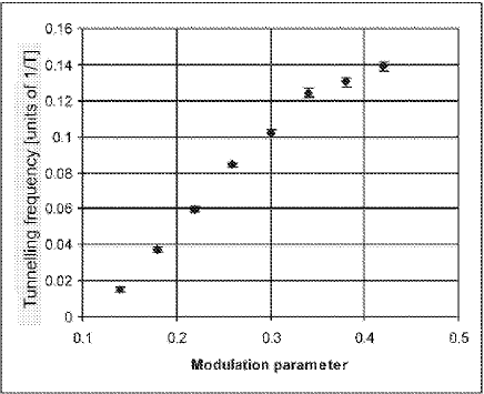
Figure 16: Tunnelling frequency as a function of the modulation parameter $\varepsilon$ (scaled well depth $\kappa=1.66,$ modulation frequency $\omega/2\pi=250$ kHz and phase shift $\varphi=0.21\cdot 2\pi$). The error bars result from the readout uncertainty of the tunnelling oscillations from the simulations. The high frequency component that is present in the data for $0.00<\varepsilon<0.18$ is not shown.

To obtain these simulations all other parameters are held constant (scaled well depth $\kappa=1.66,$ modulation frequency $\omega/2\pi=250$ kHz and phase shift $\varphi=0.21\cdot 2\pi$). For smaller values of $\varepsilon$ the corresponding classical phase space is mainly regular. There is no distinct oscillation at $\varepsilon=0.10$ which is centered at zero momentum. Distinct tunnelling oscillations start to occur at $\varepsilon=0.14$ with a gradually increasing tunnelling frequency. While there is a tunnelling period of approximately 67 modulation periods at $\varepsilon=0.14,$ the tunnelling period is only approximately 7.7 modulation periods at $\varepsilon=0.38.$ For larger values of the modulation parameter $\varepsilon$ the oscillations become less sinusoidal indicating the presence of an increasing number of dominant Floquet states. The error bars result from the readout uncertainty of the tunnelling period from the simulations.

V Moving the quantum system towards the classical limit

A fundamental strength of the experiments which are discussed here is that they are capable of exploring the transition of the quantum system towards the classical limit by decreasing the scaled Planck’s constant ${\mathchoice{\hbox{\lower 0.70007pt\hbox{$\mathchar 22\relax$}}}{\hbox{\lower 0.70007pt\hbox{$\mathchar 22\relax$}}}{\hbox{\lower 0.48996pt\hbox{$\scriptstyle\mathchar 22\relax$}}}{\hbox{\lower 0.35004pt\hbox{$\scriptscriptstyle\mathchar 22\relax$}}}\mkern-8.0muk}$.

Here a quantum system with mixed phase space exhibiting classically chaotic and regular regions of motion is moved towards the classical limit. By adjusting the scaled Planck’s constant ${\mathchoice{\hbox{\lower 0.70007pt\hbox{$\mathchar 22\relax$}}}{\hbox{\lower 0.70007pt\hbox{$\mathchar 22\relax$}}}{\hbox{\lower 0.48996pt\hbox{$\scriptstyle\mathchar 22\relax$}}}{\hbox{\lower 0.35004pt\hbox{$\scriptscriptstyle\mathchar 22\relax$}}}\mkern-8.0muk}$ of the system, the wave and particle character of the atoms can be probed although some experimental and numerical restrictions limit the extent of this quantum-classical probe. This should enhance our understanding of nonlinear dynamical systems and provide insight into their quantum and classical origin. It is out of the scope of this paper to present anything more than a short analysis relevant to the experimental results. The quantum-classical borderland is analyzed by considering the mean momentum as a function of the interaction time with the modulated standing wave for different values of the scaled Planck’s constant ${\mathchoice{\hbox{\lower 0.70007pt\hbox{$\mathchar 22\relax$}}}{\hbox{\lower 0.70007pt\hbox{$\mathchar 22\relax$}}}{\hbox{\lower 0.48996pt\hbox{$\scriptstyle\mathchar 22\relax$}}}{\hbox{\lower 0.35004pt\hbox{$\scriptscriptstyle\mathchar 22\relax$}}}\mkern-8.0muk}$. Figure 17 shows results for modulation parameter $\varepsilon=0.29,$ scaled well depth $\kappa=1.66$ and phase shift $\varphi=0.21\cdot 2\pi$ which corresponds to experimental results shown in Fig. 2. The scaled Planck’s constant ${\mathchoice{\hbox{\lower 0.70007pt\hbox{$\mathchar 22\relax$}}}{\hbox{\lower 0.70007pt\hbox{$\mathchar 22\relax$}}}{\hbox{\lower 0.48996pt\hbox{$\scriptstyle\mathchar 22\relax$}}}{\hbox{\lower 0.35004pt\hbox{$\scriptscriptstyle\mathchar 22\relax$}}}\mkern-8.0muk}$ is varied by adjusting the modulation frequency $\omega/2\pi$ and leaving the scaled well depth $\kappa,$ the modulation parameter $\varepsilon$ and the initial phase shift $\varphi$ constant. Results are shown for the scaled Planck’s constant ${\mathchoice{\hbox{\lower 0.70007pt\hbox{$\mathchar 22\relax$}}}{\hbox{\lower 0.70007pt\hbox{$\mathchar 22\relax$}}}{\hbox{\lower 0.48996pt\hbox{$\scriptstyle\mathchar 22\relax$}}}{\hbox{\lower 0.35004pt\hbox{$\scriptscriptstyle\mathchar 22\relax$}}}\mkern-8.0muk}$ ranging from 0.40 ($\omega/2\pi=500$ kHz) to 1.33 ($\omega/2\pi=150$ kHz). The error bars result from the readout uncertainty of the tunnelling period from the simulations.

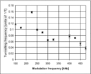
Figure 17: Dominant tunnelling frequency as a function of the modulation frequency $\omega/2\pi$ for modulation parameter $\varepsilon=0.29,$ scaled well depth $\kappa=1.66$ and phase shift $\varphi=0.21\cdot 2\pi$ which corresponds to experimental results shown in Fig. 2. As expected, the overall tendency consists of a decreasing of the tunnelling frequency as the modulation frequency increases and therefore as the scaled Planck’s constant decreases, however the transition is not as smooth as one might expect.

As shown in previous work Hensinger et al. (2001c), the momentum of the regions of regular motion is proportional to the modulation frequency. Note that this is a purely classical feature that would disappear if the scaled momentum would be plotted instead of the real momentum. Intuitively one would expect the tunnelling frequency to decrease as the system becomes more classical. However, a different quite surprising phenomenon occurs. Considering the modulation frequency interval between 225 kHz and 325 kHz the tunnelling frequency gradually decreases as the system becomes more classical. The same applies for the interval between 150 kHz to 175 kHz and the interval from 425 kHz to 475 kHz. Qualitative changes occur at approximately 200 kHz, 350 kHz (375 kHz) and 500 kHz where the tunnelling oscillation shows first multi-frequency contributions and is then significantly increased as the effective Planck’s constant is further decreased. A more detailed analysis will be subject of future study. The three intervals where the tunnelling frequency decreases appear as three arms in the graph. At $\omega/2\pi=200$ kHz, 350 kHz and 375 kHz the system cannot be well described using one dominant tunnelling frequency, therefore no data is shown at these frequencies.

The results of this first analysis indicate that the transition from quantum to classical physics contains many fascinating details to be explored. The results for the driven pendulum in atom optics shows that the transition from quantum to classical dynamics is not smooth.

VI Conclusion

Recent dynamical tunnelling experiments Hensinger et al. (2001a) were analyzed using simulations of the Gross-Pitaevskii equation and the corresponding Floquet theory. The main features of the experiments can be explained by a two or three state framework that is provided by Floquet theory. We have identified the relevant Floquet states and shown their Husimi functions. Note that the mean-field interaction was negligible in the experiments. Tunnelling period and amplitude are in good agreement with GP simulation and Floquet theory.

An analysis of the parameter space has shown that tunnelling frequency is strongly dependent on the system parameters scaled well depth $\kappa,$ modulation parameter $\varepsilon$ and the scaled Planck’s constant ${\mathchoice{\hbox{\lower 0.70007pt\hbox{$\mathchar 22\relax$}}}{\hbox{\lower 0.70007pt\hbox{$\mathchar 22\relax$}}}{\hbox{\lower 0.48996pt\hbox{$\scriptstyle\mathchar 22\relax$}}}{\hbox{\lower 0.35004pt\hbox{$\scriptscriptstyle\mathchar 22\relax$}}}\mkern-8.0muk}$. While we find an approximately linear dependence of the tunnelling frequency on the modulation parameter $\varepsilon$ for the set of experimental parameters, there is a distinct spike in the tunnelling frequency as a function of the scaled well depth $\kappa.$

However this cannot be interpreted as a signature of chaos-assisted tunnelling essentially because the states cannot be clearly identified with chaotic or regular regions of the classical phase space, therefore the notion of chaos-assisted tunnelling is difficult to use in this context. We note that it is important to decrease the scaled Planck’s constant by at least an order of magnitude Mouchet and Delande (2003) for an observation of chaos-assisted tunnelling to be non-ambiguous. We have simulated when the system is moved towards the classical limit. A bifurcation-like behavior results which can be understood in terms of quantum bifurcations of the contributing Floquet states.

VII Acknowledgements

This work was supported by the Australian Research Council. The experimental results that are shown here were accomplished by W. K. Hensinger, H. Häffner, A. Browaeys, N. R. Heckenberg, K. Helmerson, C. McKenzie, G. J. Milburn, W. D. Phillips, S. L. Rolston, H. Rubinsztein-Dunlop, and B. Upcroft in the context of reference Hensinger et al. (2001a) and we would like to thank the authors. The corresponding author W. K. H. would like to acknowledge interesting discussions with William D. Phillips and Steven Rolston during the preparation of theoretical results presented in this article. W. K. H. would like to thank NIST and Laboratoire Kastler-Brossel for hospitality during part of the work for this paper. Laboratoire Kastler Brossel de l’Université Pierre et Marie Curie et de l’Ecole Normale Supérieure is Unité Mixte de Recherche 8552 du CNRS. Laboratoire de mathématiques et de physique théorique de l’Université François Rabelais is Unité Mixte de Recherche 6083 du CNRS.

References

- Hensinger et al. (2001a) W. K. Hensinger, H. Häffner, A. Browaeys, N. R. Heckenberg, K. Helmerson, C. McKenzie, G. J. Milburn, W. D. Phillips, S. L. Rolston, H. Rubinsztein-Dunlop, et al., Nature 412, 52 (2001a).
- Hensinger et al. (2003) W. K. Hensinger, N. R. Heckenberg, G. J. Milburn, and H. Rubinsztein-Dunlop, J. Opt. B: Quantum Semiclass. Opt. 5, R83 (2003).
- Steck et al. (2001) D. A. Steck, W. H. Oskay, and M. G. Raizen, Science 293, 274 (2001).
- Steck et al. (2002) D. A. Steck, W. H. Oskay, and M. G. Raizen, Phys. Rev. Lett. 88, 120406 (2002).
- Luter and Reichl (2002) R. Luter and L. E. Reichl, Phys. Rev. A 66, 053615 (2002).
- Averbukh et al. (2002) V. Averbukh, S. Osovski, and N. Moiseyev, Phys. Rev. Lett. 89, 253201 (2002).
- Moore et al. (1995) F. L. Moore, J. C. Robinson, C. F. Bharucha, B. Sundaram, and M. G. Raizen, Phys. Rev. Lett. 75, 4598 (1995).
- Dalfovo et al. (1999) F. Dalfovo, S. Giorgini, L. P. Pitaevskii, and S. Stringari, Rev. Mod. Phys. 71, 463 (1999).
- Parkins and Walls (1997) A. S. Parkins and D. F. Walls, Phys. Rep. 303, 1 (1997).
- Dyrting et al. (1993) S. Dyrting, G. J. Milburn, and C. A. Holmes, Phys. Rev. E 48, 969 (1993).
- Mouchet et al. (2001) A. Mouchet, C. Miniatura, R. Kaiser, B. Grémaud, and D. Delande, Phys. Rev. E 64, 016221 (2001).
- Berry (1978) M. V. Berry, in Topics in Nonlinear Dynamics — A Tribute to Sir Edward Bullard, edited by Siebe and Jorna (1978), vol. 46, pp. 16–120, ISBN 0-88318-145-2, reprinted in Mackay and Meiss (1987).
- Arnold (1979) V. I. Arnold, Mathematical methods of classical mechanics (Springer-Verlag, New York, 1979).
- Ashcroft and Mermin (1976) N. W. Ashcroft and N. D. Mermin, Solid State Physics (Saunders College Philadelphia, 1976).
- Klauder and Skagerstam (1985) J. R. Klauder and B.-S. Skagerstam, Coherent States—Applications in Physics and Mathematical Physics (World Scientific, Singapore, 1985), ISBN 9971-966-52-0.
- Cohen-Tannoudji et al. (1977) C. Cohen-Tannoudji, B. Diu, and F. Laloë, Quantum mechanics (Wiley-Interscience, 1977).
- Denschlag et al. (2002) J. H. Denschlag, J. E. Simsarian, H. Häffner, C. McKenzie, A. Browaeys, D. Cho, K. Helmerson, S. L. Rolston, and W. D. Phillips, J. Phys. B - At. Mol. Opt. 35, 3095 (2002).
- Mouchet and Delande (2003) A. Mouchet and D. Delande, Phys. Rev.E 67, 046216 (2003).
- Brodier et al. (2001) O. Brodier, P. Schlagheck, and D. Ullmo, Phys. Rev. Lett. 87, 064101 (2001).
- Hensinger et al. (2001b) W. K. Hensinger, B. Upcroft, C. A. Holmes, N. R. Heckenberg, G. J. Milburn, and H. Rubinsztein-Dunlop, Phys. Rev. A 64, 063408 (2001b).
- Hensinger et al. (2001c) W. K. Hensinger, A. G. Truscott, B. Upcroft, M. Hug, H. M. Wiseman, N. R. Heckenberg, and H. Rubinsztein-Dunlop, Phys. Rev. A 64, 033407 (2001c).
- Mackay and Meiss (1987) R. S. Mackay and J. D. Meiss, Hamiltonian Dynamical Systems (Adam Hilger, Bristol and Philadelphia, 1987), ISBN 0-85274-205-3.