Detecting order and chaos in Hamiltonian systems by the SALI method

Abstract

We use the Smaller Alignment Index (SALI) to distinguish rapidly and with certainty between ordered and chaotic motion in Hamiltonian flows. This distinction is based on the different behavior of the SALI for the two cases: the index fluctuates around non–zero values for ordered orbits, while it tends rapidly to zero for chaotic orbits. We present a detailed study of SALI’s behavior for chaotic orbits and show that in this case the SALI exponentially converges to zero, following a time rate depending on the difference of the two largest Lyapunov exponents $\sigma_{1}$, $\sigma_{2}$ i.e. $\mbox{SALI}\propto e^{-(\sigma_{1}-\sigma_{2})t}$. Exploiting the advantages of the SALI method, we demonstrate how one can rapidly identify even tiny regions of order or chaos in the phase space of Hamiltonian systems of 2 and 3 degrees of freedom.

1 Introduction

Knowing whether the orbits of a dynamical system are ordered or chaotic is fundamental for the understanding of the behavior of the system. In the dissipative case, this distinction is easily made as both types of motion are attracting. In conservative systems, however, distinguishing between order and chaos is often a delicate issue (e.g. when the chaotic or ordered regions are small) especially in systems with many degrees of freedom where one cannot easily visualize the dynamics. For this reason it is of great importance to have quantities that determine if an orbit is ordered or chaotic, independent of the dimension of its phase space.

The well–known and commonly used method for this purpose is the evaluation of the maximal Lyapunov Characteristic Exponent (LCE) $\sigma_{1}$. If $\sigma_{1}>0$ the orbit is chaotic. Benettin et al. [1] studied theoretically the problem of the computation of all LCEs and proposed in [2] an algorithm for their numerical computation. In particular, $\sigma_{1}$ is computed as the limit for $t\rightarrow\infty$ of the quantity

$$L_{t}=\frac{1}{t}\,\ln\frac{|\vec{w}(t)|}{|\vec{w}(0)|}\,,\,\mbox{i.e.}\,\,\sigma_{1}=\lim_{t\rightarrow\infty}L_{t}\,,$$ (1)

where $\vec{w}(0)$, $\vec{w}(t)$ are deviation vectors from a given orbit, at times $t=0$ and $t>0$ respectively. The time evolution of $\vec{w}$ is given by solving the so–called variational equations (see Sec. 3). Generally, for almost all choices of initial deviations $\vec{w}(0)$, the limit for $t\rightarrow\infty$ of Eq. (1) gives the same $\sigma_{1}$.

In practice, of course, since the exponential growth of $\vec{w}(t)$ occurs for short time intervals, one stops the evolution of $\vec{w}(t)$ after some time $T_{1}$, records the computed $L_{T_{1}}$, normalize vector $\vec{w}(t)$ and repeats the calculation for another time interval $T_{2}$, etc. obtaining finally $\sigma_{1}$ as an average over many $T_{i}$, $i=1,2,\ldots,N$ as

$$\sigma_{1}=\frac{1}{N}\sum_{i=1}^{N}L_{T_{i}}$$

The basic problem of the computation of $\sigma_{1}$ is that, after every $T_{i}$, the calculation starts from the beginning and may yield an altogether different $L_{T_{i}}$ than the $T_{(i-1)}$ interval. Thus, since $\sigma_{1}$ is influenced by the whole evolution of $\vec{w}(0)$, the time needed for $L_{t}$ (or the $L_{T_{i}}$) to converge is not known a priori and may become extremely long. This makes it often difficult to tell whether $\sigma_{1}$ finally tends to a positive value (chaos) or converges to zero (order).

In recent years, several methods have been introduced which try to avoid this problem by studying the evolution of deviation vectors, some of which are briefly discussed in Sec. 5. In the present paper, we focus our attention on the method of the Smaller Alignment Index (SALI) [3], performing a systematic study of its behavior in the case of autonomous Hamiltonian systems with 2 (2D) and 3 (3D) degrees of freedom. This method has been applied successfully to several 2–dimensional (2d) and multidimensional maps [3], where SALI was found to converge rapidly to zero for chaotic orbits, while it exhibits small fluctuations around non–zero values for ordered orbits. It is exactly this “opposite” behavior of the SALI which makes it an ideal indicator of chaoticity: Unlike the maximal LCE, it does not start at every step a new calculation of the deviation vectors, but takes into account information about their convergence on the unstable manifold from all the previous steps. The method has already been used successfully as a chaos detection tool in some specific Hamiltonian systems [4, 5, 6, 7, 8, 9], although some authors [8, 9] use different names for the SALI.

The paper is organized as follows: In Sec. 2 we recall the definition of the SALI and present results distinguishing between ordered and chaotic motion in 2 and 3–degrees of freedom (2D and 3D) Hamiltonians, comparing also the efficiency of the SALI with the computation of $\sigma_{1}$. In Sec. 3 we explain the behavior of the SALI for ordered and chaotic orbits, showing that in the latter case SALI converges exponentially to zero following a rate which depends on the difference of the two largest Lyapunov exponents $\sigma_{1}$ and $\sigma_{2}$. In Sec. 4 we demonstrate the ability of the method to reveal the detailed structure of the dynamics in the phase space. In Sec. 5 we compare the SALI method with some other known methods of chaos detection and in Sec. 6 we summarize our results.

2 Application of the SALI in Hamiltonian systems

The basic idea behind the success of the SALI method [3] is the introduction of a simple quantity that clearly indicates if a deviation vector is aligned with the direction of the eigenvector which corresponds to the maximal LCE. In general, any two randomly chosen initial deviation vectors $\vec{w}_{1}(0)$, $\vec{w}_{2}(0)$ will become aligned with the most unstable direction and the angle between them will rapidly tend to zero [2]. Thus, we check if the two vectors have the same direction in phase space, which is equivalent to the computation of the above–mentioned angle.

More specifically, we follow simultaneously the time evolution of an orbit with initial condition $\vec{x}(0)$ and two deviation vectors with initial conditions $\vec{w}_{1}(0)$, $\vec{w}_{2}(0)$. As we are only interested in the directions of these two vectors we normalize them, at every time step, keeping their norm equal to 1. This controls the exponential increase of the norm of the vectors and avoids overflow problems. Since, in the case of chaotic orbits the normalized vectors point to the same direction and become equal or opposite in sign, the minimum of the norms of their sum (antiparallel alignment index) or difference (parallel alignment index) tends to zero. So the SALI is defined as:

$$\mbox{SALI}(t)=\min\left\{\left\|\frac{\vec{w}_{1}(t)}{\|\vec{w}_{1}(t)\|}+\frac{\vec{w}_{2}(t)}{\|\vec{w}_{2}(t)\|}\right\|,\left\|\frac{\vec{w}_{1}(t)}{\|\vec{w}_{1}(t)\|}-\frac{\vec{w}_{2}(t)}{\|\vec{w}_{2}(t)\|}\right\|\right\},$$ (2)

where $t$ is the time and $\|\cdot\|$ denotes the Euclidean norm. From the above definition is evident that $\mbox{SALI}(t)\in[0,\sqrt{2}]$ and when $\mbox{SALI}=0$ the two normalized vectors have the same direction, being equal or opposite.

In order to apply the SALI method to Hamiltonian systems, we shall use here two simple examples with 2 and 3 degrees of freedom: the well–known 2D Hénon–Heiles system [10], having the Hamiltonian function:

$$H_{2}=\frac{1}{2}(p_{x}^{2}+p_{y}^{2})+\frac{1}{2}(x^{2}+y^{2})+x^{2}y-\frac{1}{3}y^{3},$$ (3)

with equations of motion:

$$\ddot{x}=-x-2xy\,,\,\,\,\ddot{y}=-y-x^{2}+y^{2}\,,$$ (4)

and the 3D Hamiltonian system:

$$H_{3}=\frac{1}{2}(p_{x}^{2}+p_{y}^{2}+p_{z}^{2})+\frac{1}{2}(Ax^{2}+By^{2}+Cz^{2})-\epsilon xz^{2}-\eta yz^{2},$$ (5)

with equations

$$\ddot{x}=-Ax+\epsilon z^{2}\,,\,\,\,\ddot{y}=-By+\eta z^{2}\,,\,\,\,\ddot{z}=-Cx+2z(\epsilon x+\eta y)\,,$$ (6)

studied in [11, 12]. We keep the parameters of the two systems fixed at the energies $H_{2}=0.125$ and $H_{3}=0.00765$, with $A=0.9$, $B=0.4$, $C=0.225$, $\epsilon=0.56$ and $\eta=0.2$.

A simple qualitative way of studying the dynamics of a Hamiltonian system is by plotting the successive intersections of the orbits with a Poincaré surface of section (PSS) [13]. This method has been extensively applied to 2D Hamiltonians, as in these systems the PSS is a 2–dimensional plane. In 3D systems however, the PSS is 4–dimensional and the behavior of the orbits cannot be easily visualized. One way to overcome this problem is to project the PSS to spaces with lower dimensions (see e.g. [14, 15]). However, even these projections are often very complicated and difficult to interpret.

In order to illustrate the behavior of the SALI in 2D and 3D systems we first consider some representative ordered and chaotic orbits. In Fig. 1(a)

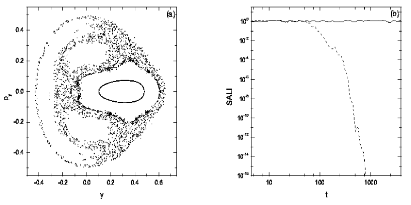
Figure 1: (a) The PSS of an ordered and a chaotic orbit with initial conditions $x=0$, $y=0.1$, $p_{x}\simeq 0.49058$, $p_{y}=0$ and $x=0$, $y=-0.25$, $p_{x}\simeq 0.42081$, $p_{y}=0$ respectively, for the Hénon–Heiles system (3). The ordered orbit corresponds to a closed (solid) elliptic curve, while the chaotic one is represented by the dots scattered over the PSS. (b) The time evolution of the SALI for the two orbits of panel (a) in log-log scale. The solid line corresponds to the ordered orbit while the dashed line corresponds to the chaotic orbit.

we plot the intersection points of an ordered and a chaotic orbit of Eqs. (4), with a PSS defined by $x=0$. The points of the ordered orbit lie on a torus and form a smooth closed curve on the PSS. On the other hand, the points of the chaotic orbit appear randomly scattered. The time evolution of the SALI for these two orbits is plotted in Fig. 1(b). In the case of the ordered orbit (solid line) the SALI remains different from zero, while in the case of the chaotic orbit (dashed line), after a small transient time, the SALI falls abruptly to zero. At $t\approx 800$ the SALI becomes zero as it has reached the limit of the accuracy of the computer ($10^{-16}$), which means that the two deviation vectors have the same direction. Thus, after $t\approx 800$ the two normalized vectors are represented by exactly the same numbers in the computer and we can safely argue, that to this accuracy the orbit is chaotic. Actually, we could conclude that the orbit is chaotic even sooner, considering that the directions of the two vectors practically coincide when the SALI reaches a small value, e.g. $10^{-8}$ after some $400$ time units. Entirely analogous behavior of the SALI distinguishes between ordered and chaotic orbits of the 3D Hamiltonian (5), as shown in Fig. 2.

Figure 2: The time evolution of the SALI for an ordered (solid line) and a chaotic orbit (dashed line) of the 3D Hamiltonian (5), with initial conditions $x=0.01054$, $y=0.05060$, $z=0$, $p_{x}=0$, $p_{y}=0$, $p_{z}\simeq 0.11906$ and $x=-0.07310$, $y=0$, $z=0$, $p_{x}=0.07695$, $p_{y}=0$, $p_{z}\simeq 0.06760$ respectively.

The initial deviation vectors, $\vec{w}=(dx,dy,dp_{x},dp_{y})$, used for both orbits of Fig. 1 are $\vec{w}_{1}(0)=(1,0,0,0)$, $\vec{w}_{2}(0)=(0,0,1,0)$, but in general any other initial choice leads to similar behavior of the SALI. The validity of the above statement is supported by the following computations. Focusing our attention on the more interesting case of chaotic motion we study the chaotic orbit of Fig. 1 by fixing one of the initial deviation vectors, keeping it e. g. $\vec{w}_{1}(0)=(0,1,0,0)$ and varying the second one $\vec{w}_{2}(0)$. For every different pair of initial vectors $\vec{w}_{1}(0)$, $\vec{w}_{2}(0)$ we compute the time $T$ needed for the SALI to become smaller than a very small value e. g. $10^{-12}$ and check if the value of $T$ depends on the particular choice of initial deviation vectors. We choose $\vec{w}_{2}(0)$ in two different ways. Firstly we consider the two initial vectors to be on the PSS of Fig. 1 having an angle $\theta$ between them so that $\vec{w}_{2}(0)=(0,\cos\theta,0,\sin\theta)$. In Fig. 3(a)

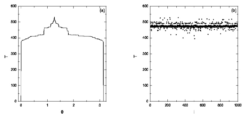
Figure 3: The time $T$ needed for the SALI to become less than $10^{-12}$ in the case of the chaotic orbit of Fig. 1 when we use as initial deviation vectors $\vec{w}_{1}(0)=(0,1,0,0)$ and (a) $\vec{w}_{2}(0)=(0,\cos\theta,0,\sin\theta)$, and (b) $\vec{w}_{2}(0)$ being a random vector. $T$ is plotted as a function of $\theta$ in (a), and as a function of a counter $i$ of the randomly generated vectors in (b).

we plot $T$ as a function of $\theta$ for $\theta\in[0,\pi]$. As expected $T=0$ for $\theta=0$ and $\theta=\pi$ since the two vectors are initially aligned. The maximum value of $T$ for $\theta\approx 0.405\pi$ corresponds to the case of $\vec{w}_{2}(0)$ being almost perpendicular to the unstable manifold which passes near the initial condition of the orbit. In this case the component of $\vec{w}_{2}(0)$ along the unstable direction is almost zero and thus, the time needed for the vector to develop a significant component along this direction, which will eventually lead it to align with the other deviation vector, is maximized. We remark that for all $\theta\in(0,\pi)$ $T$ does not change significantly, as it practically varies between 400 and 500 time units. As there is no reason for $\vec{w}_{1}(0)$, $\vec{w}_{2}(0)$ to be on the PSS the second test we perform is to compute $T$ for 1000 $\vec{w}_{2}(0)$ whose coordinates are randomly generated numbers (Fig. 3b). From the results of Fig. 3 we see that $T$ practically does not depend on choice of the initial deviation vectors.

On the other hand, the computation of the maximal LCE, using Eq. (1), despite its usefulness in many cases, does not have the same convergence properties over the same time interval. This becomes evident in Fig. 4

Figure 4: The time evolution of (a) the $L_{t}$ and (b) the SALI for the chaotic orbit $x=0$, $y=-0.01597$, $p_{x}\simeq 0.49974$, $p_{y}=0$ of the 2D system (3).

where we plot the evolution of the $L_{t}$ (panel (a)) and the SALI (panel (b)) for a chaotic orbit of Eqs. (4). At $t\approx 1900$ the SALI reaches the value $10^{-16}$ and no further computations are needed. Of course we could be sure for the chaotic nature of the orbit before that time, for example at $t\approx 1000$ (where the $\mbox{SALI}\approx 10^{-8}$). On the other hand, the computation of the $L_{t}$ (Fig. 4(a)) up to $t\approx 1000$ or even up to $t\approx 1900$, still shows no clear evidence of convergence. Although Fig. 4(a) suggests that the orbit might probably be chaotic, it does not allows us to conclude its chaotic nature with certainty, and so further computations of $L_{t}$ are needed. Thus, it becomes evident that an advantage of the SALI, with respect to the computation of $L_{t}$, is that the current value of the SALI is sufficient to determine the chaotic nature of an orbit, in contrast to the maximal LCE where the whole evolution of the deviation vector affects the computed value of $L_{t}$.

3 The behavior of the SALI for ordered and chaotic motion

As we have seen for ordered orbits the SALI remains different from zero fluctuating around some non–zero value. The behavior of the SALI for ordered motion was studied and explained in detail in the case of a completely integrable 2D Hamiltonian [16], in which no chaotic orbits exist. It was shown that any pair of arbitrary deviation vectors tend to the tangent space of the torus, on which the motion is governed by 2 independent vector fields, corresponding to the 2 integrals of motion. Thus, since $\vec{w}_{1}(t)$ and $\vec{w}_{2}(t)$, in general have one component ‘along’ and one ‘across’ the torus, there is no reason why they should become aligned and thus typically end up oscillating about two different directions. This explains why the SALI does not go to zero in the case of ordered motion.

Now let us investigate the dynamics in the vicinity of chaotic orbits of a Hamiltonian system of $n$ degrees of freedom. An orbit of this system is defined by $\vec{x}=(q_{1},\,q_{2},\,\ldots,\,q_{n},\,p_{1},\,p_{2},\,\ldots,\,p_{n})$, with $q_{i}$, $p_{i}$, $i=1,\ldots,n$ being the generalized coordinates and the conjugate momenta respectively. The time evolution of this orbit is given by Hamilton’s equations of motion

$$\frac{d\vec{x}}{dt}=\vec{V}(\vec{x})=\left(\frac{\partial H}{\partial\vec{p}}\,,-\frac{\partial H}{\partial\vec{q}}\right).$$ (7)

Solving the variational equations about a solution of (7), $\vec{x}(t)$, which represents our reference orbit under investigation,

$$\frac{d\vec{w}}{dt}=M(\vec{x}(t))\,\vec{w}\,,$$ (8)

where $M=\frac{\partial\vec{V}}{\partial\vec{x}}$ is the Jacobian matrix of $\vec{V}$, we get the time evolution of an initial deviation vector $\vec{w}(t_{0})$, for sufficiently small intervals $[t_{0},t_{0}+\Delta t]$. Note now that, in this context, the eigenvalues $\lambda_{1}\geqslant\lambda_{2}\geqslant\cdots\geqslant\lambda_{2n}$ of $M$, at $t=t_{0}$, may be thought of as local Lyapunov exponents, with $\hat{e}_{1},\,\hat{e}_{2},\,\ldots,\,\hat{e}_{2n}$ the corresponding unitary eigenvectors. These eigenvalues in fact oscillate about their time averaged values, $\sigma_{1}\geqslant\sigma_{2}\geqslant\cdots\geqslant\sigma_{2n}$, which are the global LCEs of the dynamics in that region. As is well–known in Hamiltonian systems, the Lyapunov exponents of chaotic orbits are real and are grouped in pairs of opposite sign with at least two of them being equal to zero [13]. Thus, the evolution of any initial deviation vector $\vec{w}_{1}(0)$ is given by:

$$\vec{w}_{1}(t)=\sum_{i=1}^{2n}c_{i}^{(1)}\,e^{\lambda_{i}t}\,\hat{e}_{i}\,,$$ (9)

where the $c_{i}^{(1)}$ are in general complex numbers and $\lambda_{i}$, $\hat{e}_{i}$ depend on the specific location in phase space, $\vec{x}(t_{0})$, through which our orbit passes. Note that we consider here only real eigenvalues and hence real $c_{i}^{(1)}$. If some of the $\lambda_{i}$ are complex, their corresponding contribution to (9) will be oscillatory and will not affect the argument that follows.

To get a first rough idea of the way the SALI evolves, we now make some approximations on the evolution of this deviation vector. First let us assume that the $\lambda_{i}$ do not fluctuate significantly about their averaged values and hence can be approximated by them, i.e. $\lambda_{i}\approx\sigma_{i}$. Secondly, we consider that the major contribution to $\vec{w}_{1}(t)$ comes from the two largest terms of Eq. (9), so that:

$$\vec{w}_{1}(t)\approx c_{1}^{(1)}\,e^{\lambda_{1}t}\,\hat{e}_{1}\,+c_{2}^{(1)}\,e^{\lambda_{2}t}\,\hat{e}_{2}\approx c_{1}^{(1)}\,e^{\sigma_{1}t}\,\hat{e}_{1}\,+c_{2}^{(1)}\,e^{\sigma_{2}t}\,\hat{e}_{2}.$$ (10)

In this approximation, we now use (10) to derive a leading order estimate of the ratio

$$\frac{\vec{w}_{1}(t)}{\|\vec{w}_{1}(t)\|}\approx\frac{c_{1}^{(1)}\,e^{\sigma_{1}t}\,\hat{e}_{1}\,+c_{2}^{(1)}\,e^{\sigma_{2}t}\,\hat{e}_{2}}{|c_{1}^{(1)}|\,e^{\sigma_{1}t}}=s_{1}\,\hat{e}_{1}+\frac{c_{2}^{(1)}}{|c_{1}^{(1)}|}\,e^{-(\sigma_{1}-\sigma_{2})t}\,\hat{e}_{2}\,,$$ (11)

and an entirely analogous expression for a second deviation vector:

$$\frac{\vec{w}_{2}(t)}{\|\vec{w}_{2}(t)\|}\approx\frac{c_{1}^{(2)}\,e^{\sigma_{1}t}\,\hat{e}_{1}\,+c_{2}^{(2)}\,e^{\sigma_{2}t}\,\hat{e}_{2}}{|c_{1}^{(2)}|\,e^{\sigma_{1}t}}=s_{2}\,\hat{e}_{1}+\frac{c_{2}^{(2)}}{|c_{1}^{(2)}|}\,e^{-(\sigma_{1}-\sigma_{2})t}\,\hat{e}_{2}\,,$$ (12)

where $s_{i}={\rm sign}(c_{1}^{(i)})$, $i=1,\,2$.

In order to compute the SALI, as defined by (2) we add and subtract Eqs. (11) and (12) keeping the norm of the minimum of the two evaluated quantities. Thus, $\hat{e}_{1}$ does not appear in the expression of the SALI, which becomes

$$\mbox{SALI}(t)=\min\left\|\frac{\vec{w}_{1}(t)}{\|\vec{w}_{1}(t)\|}\pm\frac{\vec{w}_{2}(t)}{\|\vec{w}_{2}(t)\|}\right\|\approx\left|\frac{c_{2}^{(1)}}{|c_{1}^{(1)}|}\pm\frac{c_{2}^{(2)}}{|c_{1}^{(2)}|}\right|\,e^{-(\sigma_{1}-\sigma_{2})t}\|\hat{e}_{2}\|$$ (13)

Denoting by $c$ the positive quantity on the r.h.s of the above equation and using the fact that $\hat{e}_{2}$ is a unitary vector we get

$$\mbox{SALI}(t)\approx c\,e^{-(\sigma_{1}-\sigma_{2})t}\,.$$ (14)

Eq. (14) clearly suggests that the SALI for chaotic orbits tends to zero exponentially and the rate of this decrease is related to the two largest LCEs of the dynamics.

Let us test the validity of this result by recalling that 2D Hamiltonian systems have only one positive LCE $\sigma_{1}$, since the second largest is $\sigma_{2}=0$. So, Eq. (14) becomes for such systems:

$$\mbox{SALI}(t)\approx c\,e^{-\sigma_{1}t}\,.$$ (15)

In Fig. 5(a)

Figure 5: (a) The evolution of $L_{t}$ for the chaotic orbit with initial condition $x=0$, $y=-0.25$, $p_{x}\simeq 0.42081$, $p_{y}=0$ of the 2D system (3). (b) The SALI of the same orbit (solid line) and the function $e^{-\sigma_{1}t}$ (dashed line) for $\sigma_{1}=0.047$. Note that the t–axis is linear.

we plot in log–log scale $L_{t}$ as a function of time $t$ for a chaotic orbit of the 2D system (3). $L_{t}$ remains different from zero, which implies the chaotic nature of the orbit. Following its evolution for a sufficiently long time interval to obtain reliable estimates ($t\approx 10000$) we obtain $\sigma_{1}\approx 0.047$. In Fig. 5(b) we plot the SALI for the same orbit (solid line) using linear scale for the time $t$. Again we conclude that the orbit is chaotic as $\mbox{SALI}\approx 10^{-16}$ for $t\approx 800$. If Eq. (15) is valid, the slope of the SALI in Fig. 5(b) should be given approximately by $\sigma_{1}$, being actually $-\sigma_{1}/\ln 10$, because $\log(\mbox{SALI})$ is a linear function of $t$. As we are only interested in the slope of the SALI, we plot in Fig. 5(b) Eq. (15) for an appropriate value of $c$ (here $c=1$) and $\sigma_{1}=0.047$ (dashed line) and find that the agreement of the approximate formula (14) to the computed values of the SALI is indeed quite satisfactory.

Chaotic orbits of 3D Hamiltonian systems generally have two positive Lyapunov exponents, $\sigma_{1}$ and $\sigma_{2}$. So, for approximating the behavior of the SALI by Eq. (14), both $\sigma_{1}$ and $\sigma_{2}$ are needed. We compute $\sigma_{1}$, $\sigma_{2}$ for a chaotic orbit of the 3D system (5) as the long time estimates of some appropriate quantities $\sigma_{1t}$, $\sigma_{2t}$ by applying the method proposed by Benettin et al. [2]. The results are presented in Fig. 6(a).

Figure 6: (a) The evolution of the two Lyapunov exponents $\sigma_{1t}$, $\sigma_{2t}$ for the chaotic orbit with initial condition $x=0$, $y=0$, $z=0$, $p_{x}=0$, $p_{y}=0$, $p_{z}\simeq 0.123693$ of the 3D system (5). (b) The SALI of the same orbit (solid line) and the function $c\,e^{-(\sigma_{1}-\sigma_{2})t}$ (dashed line) for $\sigma_{1}=0.0107$, $\sigma_{2}=0.0005$ and $c=10^{5}$. Note that the t–axis is linear.

The computation is carried out until $\sigma_{1t}$ and $\sigma_{2t}$ stop having high fluctuations and approach some non–zero values (since the orbit is chaotic), which could be considered as good approximations of their limits $\sigma_{1}$, $\sigma_{2}$. Actually for $t\approx 10^{5}$ we have $\sigma_{1t}\approx 0.0107$, $\sigma_{2t}\approx 0.0005$. Using these values as good approximations of $\sigma_{1}$, $\sigma_{2}$ we see in Fig. 6(b) that the slope of the SALI (solid line) is well reproduced by Eq. (14) (dashed line). Note how much more quickly the SALI’s convergence to zero shows chaotic behavior, while the two LCEs, $\sigma_{1t}$ $\sigma_{2t}$, take a lot longer to reach their limit values. Moreover, the results presented in Figs. 5 and 6 give strong evidence for the validity of Eq. (14) in describing the behavior of the SALI for chaotic motion. So we conclude that for chaotic motion the SALI is related to the two largest Lyapunov exponents and decreases asymptotically as ${\mbox{S}ALI}\propto e^{-(\sigma_{1}-\sigma_{2})t}$.

4 Distinguishing between regions of order and chaos

The SALI offers indeed an easy and efficient method for distinguishing the chaotic vs. ordered nature of orbits in a variety of problems. In the present section we use it for identifying regions of phase space where large scale ordered and chaotic motion are both present.

In Fig. 7

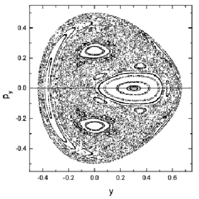
Figure 7: The PSS $x=0$ of the 2D Hénon–Heiles system (3). The axis $p_{y}=0$ is also plotted.

we present a detailed plot of the $x=0$ PSS of the 2D Hénon–Heiles system (3). Regions of ordered motion, around stable periodic orbits, are seen to coexist with chaotic regions filled by scattered points. In order to demonstrate the effectiveness of the SALI method, we first consider orbits whose initial conditions lie on the line $p_{y}=0$. In particular we take $5000$ equally spaced initial conditions on this line and compute the value of the SALI for each one. The results are presented in Fig. 8

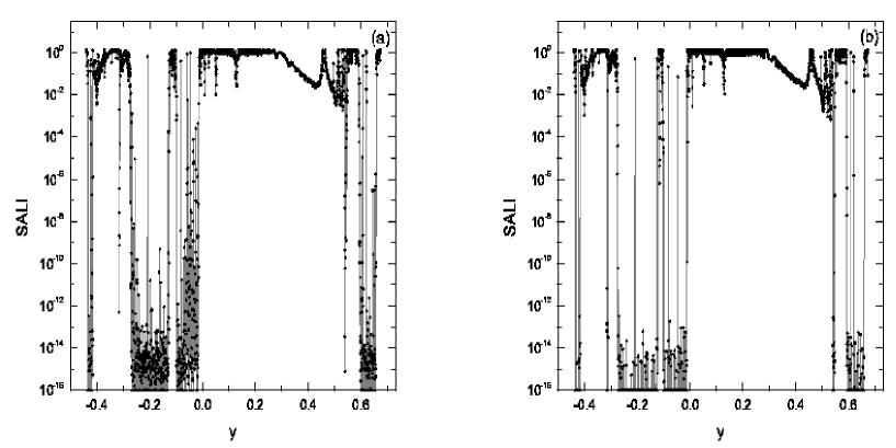
Figure 8: The values of the SALI for (a) $t=1000$ and (b) $t=4000$ for orbits of the 2D system (3) with initial conditions on the $p_{y}=0$ line on the PSS (Fig. 7), as a function of the $y$ coordinate of the initial condition.

where we plot the SALI as a function of the $y$ coordinate of the initial condition of these orbits for $t=1000$ (panel (a)) and $t=4000$ (panel (b)). In both panels the data points are line connected, so that the changes of the SALI values are clearly visible. Note that there are intervals where the SALI has large values (e.g. larger than $10^{-4}$), which correspond to ordered motion in the island of stability crossed by the $p_{y}=0$ line in Fig. 7. There also exist regions where the SALI has very small values (e.g. smaller than $10^{-12}$) denoting that in these regions the motion is chaotic. These intervals correspond to the regions of scattered points crossed by the $p_{y}=0$ line in Fig. 7. Although most of the initial conditions give large ($>10^{-4}$) or very small ($\leqslant 10^{-12}$) values for the SALI, there also exist initial conditions that have intermediate values of the SALI ($10^{-12}<\mbox{SALI}\leqslant 10^{-4}$) e.g. at $t=1000$ in Fig. 8(a). These initial conditions correspond to sticky chaotic orbits, remaining for long time intervals at the borders of islands, whose chaotic nature will be revealed later on. By comparing Figs. 8(a) and 8(b) it becomes evident that almost all points having $10^{-12}<\mbox{SALI}\leqslant 10^{-4}$ in Fig. 8(a) move downwards to very small values of the SALI in Fig. 8(b), while the intervals that correspond to ordered motion remain the same. Again in Fig. 8(b) there exist few points having intermediate values of the SALI, which correspond to sticky orbits whose SALI will eventually become zero. We note that it is not easy to define a threshold value, so that the SALI being smaller than this value reliably signifies chaoticity. Nevertheless, numerical experiments in several systems show that in general a good guess for this value could be $\lesssim 10^{-4}$.

In both panels of Fig. 8, around $y\approx-0.1$ there exists a group of points inside a big chaotic region having $\mbox{SALI}>10^{-4}$. These points correspond to orbits with initial conditions inside a small stability island, which is not even visible in the PSS of Fig. 7. Also the point with $y=-0.2088$ has very high value of the SALI ($>0.1$) in both panels of Fig. 8, while all its neighboring points have $\mbox{SALI}<10^{-9}$ even for $t=1000$. This point actually corresponds to an ordered orbit inside a tiny island of stability, which can be revealed only after a very high magnification of this region of the PSS. So, we see that the systematic application of the SALI method can reveal very fine details of the dynamics.

By carrying out the above analysis for points not only along a line but on the whole plane of the PSS, and giving to each point a color according to the value of the SALI, we can have a clear picture of the regions where chaotic or ordered motion occurs. The outcome of this procedure for the 2D Hénon–Heiles system (3), using a dense grid of initial conditions on the PSS, is presented in Fig. 9(a).

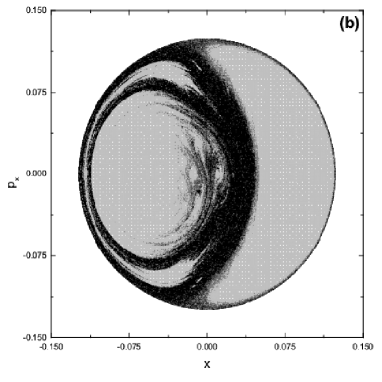
Figure 9: Regions of different values of the SALI (a) on the PSS $x=0$ of the 2D Hénon–Heiles system (3), at $t=1000$ and (b) on the subspace $y=0$, $p_{y}=0$ of the PSS $z=0$ of the 3D system (5), at $t=5000$. In both frames initial conditions are colored black if their $\mbox{SALI}\leqslant 10^{-12}$, deep gray if $10^{-12}<\mbox{SALI}\leqslant 10^{-8}$, gray if $10^{-8}<\mbox{SALI}\leqslant 10^{-4}$ and light gray if $\mbox{SALI}>10^{-4}$.

The values of the logarithm of the SALI are divided in 4 intervals. Initial conditions having different values of the SALI at $t=1000$ are plotted by different shades of gray: black if $\mbox{SALI}\leqslant 10^{-12}$, deep gray if $10^{-12}<\mbox{SALI}\leqslant 10^{-8}$, gray if $10^{-8}<\mbox{SALI}\leqslant 10^{-4}$ and light gray if $\mbox{SALI}>10^{-4}$. Thus, in Fig. 9(a) we clearly distinguish between light gray regions, where the motion is ordered and black regions, where it is chaotic. At the borders between these regions we find deep gray and gray points, which correspond to sticky chaotic orbits. It is worth–mentioning that in Fig. 9(a) we can see small islands of stability inside the large chaotic sea, which are not visible in the PSS of Fig. 7, like the one for $y\approx-0.1$, $p_{y}\approx 0$. Although Fig. 9(a) was computed for only $t=1000$ (like Fig. 8(a)), this time was sufficient for the clear revelation of small ordered regions inside the chaotic sea.

The construction of Fig. 9(a) was actually speeded up by attributing the final value of the SALI (at $t=1000$) of an orbit to all its intersection points with the PSS, and by stopping the evolution of the orbit if its SALI became equal to zero for $t<1000$. For a grid of $375\times 750$ equally spaced initial conditions on the $p_{y}\geqslant 0$ part of the figure, we need about 2 hours of CPU time on a Pentium 4 2GHz PC. Although it is difficult to estimate, we expect that it would take considerably longer to discern the same kind of detail, by straightforward integration of Eqs. (4) for a similar grid of initial conditions.

For 3D Hamiltonians the PSS is 4–dimensional and thus, not so useful as in the 2D case. On the other hand, the SALI can again identify successfully regions of order and chaos in phase space. To see this, let us start with initial conditions on a 4d grid of the PSS and attribute again the final value of the SALI of an orbit to all the points visited by the orbit. In this way, we again find regions of order and chaos, which may be visualized, if we restrict our study to a subspace of the whole 4d phase space. As an example, we plot in Fig. 9(b) the subspace $y=0$, $p_{y}=0$ of the 4d PSS $z=0$ of the 3D system (5), using the same technique as in Fig. 9(a). Again we can see regions of ordered (colored in light gray) and chaotic motion (colored in black), as well as sticky chaotic orbits (colored in deep gray and gray) at the edges of these regions. Pictures like the ones of Fig. 9, apart from presenting the regions of order and chaos, could also be used to estimate roughly the fraction of phase space volume occupied by chaotic or ordered orbits and provide good initial guesses for the location of stable periodic orbits, in regions where the motion is ordered.

5 Comparison with other methods

The results presented in the previous sections show that the SALI is a simple, efficient and easy to compute tool for distinguishing between ordered and chaotic motion. Implementing the SALI is an easy computational task as we only have to follow the evolution of an orbit and of two deviation vectors, computing in every time step the minimum norm of the difference and the addition of these vectors. In the case of chaotic motion the SALI eventually tends exponentially to zero, reaching rapidly very small values or even the limit of the accuracy of the computer. On the other hand, in the case of ordered motion the SALI fluctuates around non–zero values. It is exactly this different behavior of the SALI that makes it an ideal tool of chaos detection. The SALI has a clear physical meaning as zero, or a very small value of the index, signifies the alignment of the two deviation vectors. An advantage of the method is that the index ranges in a defined interval ($\mbox{SALI}\in[0,\sqrt{2}]$) and so very small values of the SALI (e. g. smaller than $10^{-8}$) establish the chaotic nature of an orbit beyond any doubt.

The SALI helps us decide the chaotic nature of orbits faster and with less computational effort than the estimation of the maximal LCE. This happens because the time needed for $L_{t}$ to give a clear and undoubted indication of convergence to non–zero values is usually much greater than the time in which the SALI becomes practically zero, as can be seen in Figs. 4, 5 and 6.

Many other chaos indicators have been introduced in recent years, some of which are compared in this section with the SALI. We also study in more detail the latest method we very recently became aware of, the so–called 0–1 test, introduced by Gottwald and Melbourne [17].

The efficiency of the SALI was compared in [3] with the well–known method of the Fast Lyapunov Indicator (FLI) [18, 19] and the method of the spectral distance $D$ of spectra of stretching numbers [20]. It was shown that the SALI has comparable behavior to the FLI both for ordered and chaotic orbits, with the SALI being able to decide the nature of an orbit at least as fast as the FLI. An advantage of the SALI method with respect to the FLI is the fact that the SALI ranges in a given interval, with very small values corresponding to chaotic behavior, while the values of FLI increase in time, both for ordered and chaotic motion, but with different rates. So, the interpretation of different colors in color plots produced by the SALI method, like the ones of Fig. 9, does not depend on the integration time of the orbits, in contrast to similar plots of the FLI, since the range of FLI values changes as time grows. As was explained in detail in [3] the computation of the SALI is much easier and faster than the computation of the spectral distance $D$, mainly because we do not have to go through the computation of the spectra of stretching numbers. Also the SALI can be used to distinguish between order and chaos in the case of 2d maps, where the spectral distance $D$ cannot be applied.

Sándor et al. [21] comparing the Relative Lyapunov Indicator (RLI) method with the SALI showed that both indices have similar behaviors even in cases of weakly chaotic motion. The RLI is practically the absolute value of the difference of $L_{t}$ of two initially nearby orbits, with very small values of the RLI denoting ordered motion, while large differences between the $L_{t}$’s denote chaotic behavior (for more information on the RLI method see [21]). We note that the computation of the RLI requires the time evolution of two orbits and two deviation vectors (one for each orbit), while the computation of the SALI is faster as we compute one orbit and two deviation vectors.

Very recently, Gottwald and Melbourne [17] introduced a new test for distinguishing ordered from chaotic behavior in deterministic dynamical systems: the 0–1 test. The method is quite general and can be applied directly to long time series data produced by the evolution of a dynamical system. In that sense, the 0–1 test is more general than the SALI for the computation of which we need to know the equations that govern the evolution of the system, as well as its variational equations. The 0–1 test uses the real valued function:

$$p(t)=\int_{0}^{t}\phi(s)\,\cos(\psi(s))\,ds\,\,,$$ (16)

where $\phi(s)$ is, in general, any observable of the underlying dynamics and

$$\psi(t)=kt+\int_{0}^{t}\phi(s)\,ds\,\,,$$ (17)

with $k$ being a positive constant. By defining the mean–square–displacement of p(t):

$$M(t)=\lim_{T\rightarrow\infty}\frac{1}{T}\int_{0}^{T}\left(p(t+\tau)-p(\tau)\right)^{2}\,d\tau\,\,,$$ (18)

and setting

$$K(t)=\frac{\log(M(t)+1)}{\log t}\,,$$ (19)

one takes the limit

$$K=\lim_{t\rightarrow\infty}K(t)\,,$$ (20)

and characterizes the particular orbit as ordered if $K=0$, or chaotic if $K=1$. The justification of the 0–1 test, as well as applications of the method to some dynamical systems can be found in [17].

In order to compare the 0–1 test with the SALI method we apply it in the cases of the ordered and chaotic orbits of the Hénon–Heiles system (3) presented in Fig. 1. Recall that in the case of the chaotic orbit the SALI determines the true nature of the orbit at $t\approx 800$ when $\mbox{SALI}\approx 10^{-16}$, or even at $t\approx 400$ if we consider the more loose condition that $\mbox{SALI}\approx 10^{-8}$ guarantees chaoticity. We consider as an observable $\phi(t)$ the quantity:

$$\phi(t)=y(t)+p_{y}(t)\,,$$ (21)

while for the constant $k$ we adopt the value used in [17], i. e. $k=1.7$. The application of the 0–1 test requires a rather long time series of the observable $\phi(t)$ in order to reliably compute firstly $M(t)$ for $T\rightarrow\infty$ (Eq. 18) and secondly $K$ as the limit of $K(t)$ for $t\rightarrow\infty$ (Eq. 20). In our computations we set $T=90000$ time units and compute $K(t)$ for $t\in(0,10000)$, which means that the particular orbit is integrated up to $t=10^{5}$ time units. Although the assumption $T\gg t$, which is formally required for the convergence of $K(t)$ (see [17]), is not fulfilled, the behavior of $K(t)$ for the ordered and chaotic orbit is different, allowing us to distinguish between the two cases (Fig. 10).

Figure 10: Application of the 0–1 test for the orbits of Fig. 1. $K(t)$ oscillates with an amplitude decreasing towards $K=0$ for the ordered orbit (solid line), while it tends to $K=1$ for the chaotic orbit (dashed line).

In particular, $K(t)$ increases for the chaotic orbit (dashed line in Fig. 10) showing a tendency to reach $K=1$, while it tends to $K=0$ for the ordered orbit (solid line in Fig. 10) exhibiting fluctuations of slowly decreasing amplitude. From these results it is obvious that the true nature of the orbits is determined correctly by the 0–1 test, but the computational effort needed in order to be able to characterize the orbits is much higher than in the case of the SALI. This difference is due to, firstly, the more complicated way of estimating $K$, in comparison with the computation of the SALI, as we have to compute several integrals, and secondly, the fact that we must compute the particular orbit for sufficiently long time, in order to approximate the limits of Eqs. (18), (20). Of course, as we have already mentioned, the 0–1 test is more general as it can also be readily applied to time series data, without knowing necessarily the equations of the dynamical system.

6 Summary

In this paper we have applied the SALI method to distinguish between order and chaos in 2D and 3D autonomous Hamiltonian systems, and have also analyzed the behavior of the index for chaotic orbits. Our results can be summarized as follows.

• The SALI proves to be an ideal indicator of chaoticity independent of the dimensions of the system. It tends to zero for chaotic orbits, while it exhibits small fluctuations around non–zero values for ordered ones and so it clearly distinguishes between these two cases. Its advantages are its simplicity, efficiency and reliability as it can rapidly and accurately determine the chaotic vs ordered nature of a given orbit. In regions of ‘stickiness’, of course, along the borders of ordered motion it displays transient oscillations. However, once the orbit enters a large chaotic domain the SALI converges exponentially to zero, often at shorter times than it takes the maximal Lyapunov exponent to converge to its limiting value.

• We emphasize that the main advantage of the SALI in chaotic regions is that it uses two deviation vectors and exploits at every step, their convergence to the unstable manifold from all previous steps. This allows us to show that the SALI tends to zero for chaotic orbits at a rate which is related to the difference of the two largest Lyapunov characteristic exponents $\sigma_{1}$, $\sigma_{2}$ as $\mbox{SALI}\propto e^{-(\sigma_{1}-\sigma_{2})t}$. By comparison, the computation of the maximal LCE, even though it requires only one deviation vector and one exponent, $\sigma_{1}$, often takes longer to converge, since it needs to average over many time intervals, where the calculation of this exponent is independent from all previous intervals. The SALI was also proved to have similar or even better performance than other methods of chaos detection which were briefly discussed in Sec. 5.

• The $\mbox{SALI}\in[0,\sqrt{2}]$ and its value characterize an orbit of being chaotic or ordered. Exploiting this feature of the index we have plotted detailed phase space portraits both for 2D and 3D Hamiltonian systems, where the chaotic and ordered regions are clearly distinguished. We were thus able to trace in a fast and systematic way very small islands of ordered motion, whose detection by traditional methods would be very difficult and time consuming. This approach is therefore expected to provide useful tools for the location of stable periodic orbits, or the computation of the phase space volume occupied by ordered or chaotic motion in multidimensional systems, where the PSS is not easily visualized, and very few other similar techniques of practical value are available.

References

References

- [1] Benettin G, Galgani L, Giorgilli A and Strelcyn J-M 1980 Meccanica March 9
- [2] Benettin G, Galgani L, Giorgilli A and Strelcyn J-M 1980 Meccanica March 21
- [3] Skokos Ch 2001 J. Phys. A: Math. Gen.34 10029
- [4] Skokos Ch, Antonopoulos Ch, Bountis T C and Vrahatis M N 2003 Libration Point Orbits and Applications eds G Gomez, M W Lo and J J Masdemont (Singapore: World Scientific) p 653
- [5] Panagopoulos P, Bountis T C and Skokos Ch 2004 J. Vib. & Acoust. (in press)
- [6] Széll A 2003 PhD Thesis Glasgow Caledonian University
- [7] Széll A, Érdi B, Sándor Zs and Steves B 2004 MNRAS 347 380
- [8] Voglis N, Kalapotharakos C and Savropoulos I 2002 MNRAS 337 619
- [9] Kalapotharakos C, Voglis N and Contopoulos G 2004 MNRAS (submitted)
- [10] Hénon M and Heiles C 1964 Astron. J. 69 73
- [11] Contopoulos G and Magnenat P 1985 Cel. Mech. 37 387
- [12] Contopoulos G and Barbanis B 1989 Astron. Astrophys. 222 329
- [13] Lieberman M A and Lichtenberg A J 1992 Regular and Chaotic Dynamics (Springer Verlag)
- [14] Vrahatis M N, Bountis T C and Kollmann M 1996 Int. J. Bifurc. Chaos 6 1425
- [15] Vrahatis M N, Isliker H and Bountis T C 1997 Int. J. Bifurc. Chaos 7 2707
- [16] Skokos Ch, Antonopoulos Ch, Bountis T C and Vrahatis M N 2003 Prog. Theor. Phys. Supp. 150 439
- [17] Gottwald G A and Melbourne I 2004 Proc. Roy. Soc. London A 460 603
- [18] Froeschlé C, Lega E and Gonczi R 1997 Celest. Mech. Dyn. Astron. 67 41
- [19] Froeschlé C, Gonczi R and Lega E 1997 Planet. Space Sci. 45 881
- [20] Voglis N, Contopoulos G and Efthymiopoylos C 1999 Celest. Mech. Dyn. Astron. 73 211
- [21] Sándor Zs, Érdi B, Széll A and Funk B 2004 Celest. Mech. Dyn. Astron. (in press)