Surrogate Test to Distinguish between Chaotic and Pseudoperiodic Time Series

Abstract

In this communication a new algorithm is proposed to produce surrogates for pseudoperiodic time series. By imposing a few constraints on the noise components of pseudoperiodic data sets, we devise an effective method to generate surrogates. Unlike other algorithms, this method properly copes with pseudoperiodic orbits contaminated with linear colored observational noise. We will demonstrate the ability of this algorithm to distinguish chaotic orbits from pseudoperiodic orbits through simulation data sets from the Rössler system. As an example of application of this algorithm, we will also employ it to investigate a human electrocardiogram (ECG) record.

I Introduction

Surrogate tests Theiler testing (1) are examples of Monte Carlo hypothesis tests Galka topics (4). Taking the surrogate test of nonlinearity in a time series Theiler testing (1) as an example, we first need to adopt a null hypothesis, which usually supposes the time series is generated by a linear stochastic process and potentially filtered by a nonlinear filter note nonlinearity (5). Based on this null hypothesis, a large number of data sets (surrogates) are to be produced from the original time series, which keeps the linearity of the original time series but destroys all other structures. We then calculate some nonlinear statistics (discriminating statistics), for example, correlation dimension, of both the original time series and the surrogates. If the discriminating statistic of the original time series deviates from those of the surrogates, we can reject the null hypothesis we proposed and claim that the original time series is deterministic with certain confidence level (depending on how many surrogates we have generated, to be shown later). In general, to apply the surrogate technique to test if a time series possesses the property $P$ we are interested, we first select a null hypothesis, which assumes the time series instead has a property $Q$ opposite to $P$. We then devise a corresponding algorithm to produce surrogates from the observed data set. In principle, these surrogates shall preserve the potential property $Q$ while destroying all others. The next step is to choose a suitable discriminating statistic, which shall be an invariant measure for both the surrogates and the original time series if the null hypothesis is true. Hence if the discriminating statistic of the original time series distinctly deviates from the distribution of the discriminating statistic of the surrogates, the null hypothesis is unlikely to be true, or in other words, the time series is much more likely to possess the property $P$ than $Q$. In this way, we can assess the statistical significance of our calculations through surrogate test technique even when we have only a very limited amount of observations. Such assessments are important because in many practical situations statistical fluctuations are inevitable due to the presence of noise, hence the surrogate test is a proper tool to evaluate the reliability of our results in a statistical sense.

In this communication, we are focused on discussing the algorithm to generate surrogates for pseudoperiodic time series. By pseudoperiodic time series we mean a representative of a periodic orbit perturbed by dynamical noise, or contaminated by observational noise, or with the combination of the both noises, whose states within one cycle are largely independent of those within previous cycles given a cycle length. Note that, in our discussions we will always assume we have detected that the time series are produced from nonlinear deterministic systems, but they are also possibly contaminated by some noises. As we know, if an irregular time series comes from a nonlinear deterministic system, it shall be either chaotic or pseudoperiodic in most cases. In some situations, it might be important for us to discriminate between pseudoperiodicity and chaos. However, chaotic and pseudoperiodic time series often look similar, we might not be able to distinguish them from each other only through visual inspections, quantitative techniques are needed instead at this time. One choice is to apply the direct test techniques. For instance, we can calculate some characteristic statistics of the time series, such as the Lyapunov exponent and the correlation dimension. However, a direct test usually will not give out the confidence level. If we find the Lyapunov exponent of a time series is, for example, $0.01$, it may be difficult for us to tell whether the time series is chaotic or the time series is pseudoperiodic, but the presence of noise causes the Lyapunov exponent to be slightly larger than zero. As an alternative choice, we suggest one utilizes the surrogate test rather than the direct test, which can provide us the confidence level by calculating a large number of surrogates. Through the surrogate tests, if we could exclude the possibility that the time series is pseudoperiodic, then the time series is more likely to be chaotic. This is the essential idea to apply our algorithm to distinguish chaos from pseudoperiodicity, as to be shown in section III.

First let us briefly review some of the algorithms to generate surrogates for pseudoperiodic time series. Initially, to generate surrogates for pseudoperiodic time series, Theiler Theiler on (2) proposed the cycle shuffling algorithm. The idea is to divide the whole data set into some segments and let each segment contain exactly an integer number of cycles. The surrogates are obtained by randomly shuffling these segments, which will preserve the intracycle dynamics but destroy the intercycle ones by randomizing the temporal sequence of the individual cycles. The difficulty in applying this algorithm is that it requires preknowledge of the precise periodicity, otherwise shuffling the individual cycles might lead to spurious results Small surrogate (9).

Recently, with the development of the cyclic theory of chaos Ayerbach exploring (6), many authors have shown interest in searching unstable periodic orbits (UPOs) in noisy data sets from chaotic dynamical systems. The algorithms proposed in Pierson detecting (7) essentially deal with the unstable fixed points of the UPOs. But as observed, the presence of noise will reduce the statistical significance of these algorithms. One remedy is to introduce the surrogate test for reliability assessments, e.g., Dolan et.al Pierson detecting (7) claimed that the randomly shuffling surrogate algorithm Theiler testing (1) together with the simple recurrence method Pierson detecting (7) correctly tests the appropriate null hypothesis. Essentially, this approach is very similar to the cycle shuffling algorithm described previously. The simple recurrence algorithm is equivalent to applying a Poincaré map on the continuous dynamical systems and then studying only the data points falling on the cross-section plane, hence one does not need to consider the intracycle dynamics and no knowledge of the periodicity is required, while randomly shuffling these data points exactly aims to randomize the temporal sequence of the cycles. However, one potential problem of this algorithm is that it might generate spuriously high statistical significance due to the correlation between the cycles Petracchi the (8).

Later, Small et.al Small surrogate (9) proposed the pseudoperiodic surrogate (PPS) algorithm from another viewpoint. They first apply the time delay embedding reconstruction Takens detecting (16) to the original data set, then utilize a method based on local linear modelling techniques to produce surrogate data which approximate the behavior of the underlying dynamical system. As the authors pointed out, this algorithm works well even with very large dynamical noise, but it may incorrectly reject the null hypothesis if the intercycles of the pseudoperiodic orbit have a linear stochastic dependence induced by colored additive observational noise note noise (10).

In this communication we propose a new surrogate algorithm for continuous dynamical systems, which properly copes with linear stochastic dependence between the cycles of the pseudoperiodic orbits. The null hypothesis to be tested is that the stationary data set is pseudoperiodic with noise components which are (approximately) identically distributed and uncorrelated for sufficiently large temporal translations. Note the constraints of the noise components in our null hypothesis are stronger than that of Theiler’s algorithm, which requires the noise distribution only periodically depends on the phase of the signal. However, under our hypothesis, we can produce the surrogates in a simple way through the algorithm to be described below. In addition, a large scope of noise processes often encountered in practical situations, including (but not limited to) linear colored additive observational noise described by the $ARMA(p,q)$ model Box time (15), match the above constraints.

The remainder of this communication is organized as follows. In Sec. II we will introduce the new algorithm to generate pseudoperiodic surrogates, while in Sec. III we will apply this algorithm to simulation data sets from the Rössler system, which demonstrates the ability of the surrogate test based on this algorithm to distinguish chaotic orbits from pseudoperiodic ones. As one of the applications, we will use this surrogate technique to investigate whether a human electrocardiogram (ECG) record is possibly presentative of a chaotic dynamical system. Finally, in Sec. IV, we will have a summary of the whole communication.

II A New Algorithm to Generate Pseudoperiodic Surrogates

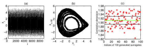
Figure 1: (a) Pseudoperiodic time series contaminated by observational noise; (b) State space $x_{i+n}$ vs. $x_{i}$ of the pseudoperiodic time series from the Rössler system with $n=16$; (c) Surrogate test for the pseudoperiodic time series based on our algorithm. The abscissa is the indices of 100 surrogates and the ordinate is the corresponding correlation dimensions. The middle line is the mean correlation dimension of the original time series calculated $100$ times using the GKA, the upper and lower lines denote the correlation dimensions twice the standard deviation away from the mean value and the asterisks indicate the correlation dimensions of $100$ surrogates.

Let $\left\{x_{i}\right\}_{i=1}^{N}$ be a data set with $N$ observations (the form $\left\{x_{i}\right\}$ is adopted instead for convenience when causing no confusion), where $x_{i}$ means the observation measured at time $t_{i}=i\cdot\Delta t_{s}$ with $\Delta t_{s}$ denoting the sampling time. We assume $\left\{x_{i}\right\}_{i=1}^{N}$ is stationary and can be decomposed into the deterministic components and the noise components, which are approximately independent of each other. Similar to the surrogate test idea of time shifting to desynchronize two data sets quiroga performance (12), we assume the noise components (approximately) follow an identical distribution and are uncorrelated for sufficiently large temporal translations (or time shifts). According to the null hypothesis we proposed in the previous section, if the deterministic components are periodic, then we can write a data point $x_{i}$ as $x_{i}=p_{i}+n_{i}$, where $p_{i}$ and $n_{i}$ denote the periodic component and the noise component respectively. In many cases, we can set $E(p_{i})=E(n_{i})=0$ where $E$ is the expectation operator. Since $\left\{p_{i}\right\}$ are roughly independent of $\left\{n_{i}\right\}$, we have the autocovariance $var(x_{i})=var(p_{i})+var(n_{i})$. Let

$$y_{i}^{\tau}=\alpha x_{i}+\beta x_{i+\tau}=(\alpha p_{i}+\beta p_{i+\tau})+(\alpha n_{i}+\beta n_{i+\tau})$$ (1)

with $i=1,2,~{}...,N-\tau$, where coefficients $\alpha$ and $\beta$ satisfy $\alpha^{2}+\beta^{2}=1$ and parameter $\tau$ is the temporal translation between subsets $\left\{x_{i}\right\}_{i=1}^{N-\tau}$ and $\left\{x_{i+\tau}\right\}_{i=1}^{N-\tau}$, then the autocovariance function $var(y_{i}^{\tau})=var(\alpha p_{i}+\beta p_{i+\tau})+var(\alpha n_{i}+\beta n_{i+\tau})$. Now let us consider the noise components. If $\tau$ is sufficiently large, under our hypothesis, $n_{i}$ and $n_{i+\tau}$ are uncorrelated. We also note that $\left\{n_{i}\right\}$ and $\left\{n_{i+\tau}\right\}$ are drawn from (approximately) the same distribution, we have $var(\alpha n_{i}+\beta n_{i+\tau})=var(n_{i})$. For the deterministic component, if we require the translation $\tau$ to satisfy $cov(p_{i},p_{i+\tau})=0$, then $var(\alpha p_{i}+\beta p_{i+\tau})=var(p_{i})$. Hence by choosing a suitable temporal translation, the noise levels of $\left\{y_{i}^{\tau}\right\}$, defined by $\left(var(\alpha n_{i}+\beta n_{i+\tau})/var(y_{i}^{\tau})\right)^{1/2}$, will be the same as that of $\left\{x_{i}\right\}_{i=1}^{N}$, i.e., $\left(var(n_{i})/var(x_{i})\right)^{1/2}$. The reason to preserve the noise level is that, the presence of noise will affect the calculation of the correlation dimension, hence we would like to let the surrogates and the original time series (roughly) have the same noise level in order to make the results more conceivable.

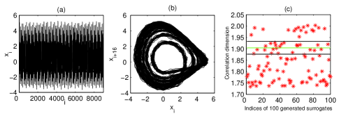
Figure 2: (a) Pseudoperiodic time series with both observational noise and dynamical noise; (b) State space $x_{i+n}$ vs. $x_{i}$ of the pseudoperiodic time series from the Rössler system with $n=16$; (c) Surrogate test for the pseudoperiodic time series based on our algorithm. The meaning of the lines and the asterisks is the same as that in panel $(c)$ of Fig. 1.

The above deduction leads to the central idea of our surrogate algorithm. From Eq. (1), we note that if $\left\{p_{i}\right\}$ is periodic, the nonconstant deterministic components $\left\{\alpha p_{i}+\beta p_{i+\tau}\right\}$ shall also be periodic. In addition, $\left\{x_{i}\right\}_{i=1}^{N}$ and $\left\{y_{i}^{\tau}\right\}$ shall have the same noise level if a suitable translation $\tau$ is selected. Therefore by randomizing the coefficient $\alpha$ or $\beta$, we can generate many data sets $\left\{y_{i}^{\tau}\right\}$ as the surrogates of $\left\{x_{i}\right\}_{i=1}^{N}$. Note that $\left\{p_{i}\right\}$ and $\left\{\alpha p_{i}+\beta p_{i+\tau}\right\}$ have the same degree-of-freedom, if both of them are periodic, their correlation dimensions Grassberger characterization (13) will theoretically be the same. Now let us consider the noise components. Although the noise components $\left\{\alpha n_{i}+\beta n_{i+\tau}\right\}$ may have a different distribution from that of $\left\{n_{i}\right\}$, the noise level is preserved after the transform in Eq. (1). As Diks Diks estimating (20) has reported, the Gaussian kernel algorithm (GKA) can reasonably estimate the correlation dimensions of noisy data sets with different noise distributions. This implies that, under the same noise level, the correlation dimensions of $\left\{x_{i}\right\}_{i=1}^{N}$ and $\left\{y_{i}^{\tau}\right\}$, calculated by the GKA, shall statistically be the same if $\left\{x_{i}\right\}_{i=1}^{N}$ and $\left\{y_{i}^{\tau}\right\}$ are both pseudoperiodic (and satisfy the constraints we imposed). In contrast, if $\left\{p_{i}\right\}$ is chaotic, its linear combination, $\left\{\alpha p_{i}+\beta p_{i+\tau}\right\}$, may have a new dynamical structure with a different correlation dimension from that of $\left\{p_{i}\right\}$, hence by adopting the correlation dimension as the discriminating statistic we might detect this difference.

We shall also note that, for an unstable periodic orbit, even a small dynamical noise might drive the resultant orbit far away from the original position after a sufficiently long time, and the pseudoperiodicity might be broken. In such situations, our algorithm might fail to work. Nevertheless, we suggest to apply our algorithm as the first step in pseudoperiodicity test, which is computationally fast and in principle deals well with a large scope of observational noise (comparatively, the PPS algorithm will sometimes fail for colored observational noise). If we can reject the null hypothesis proposed previously, the time series in test is possibly chaotic or pseudoperiodic perturbed by dynamical noise. Then we can adopt the PPS algorithm for further tests, which works well even under a large amount of dynamical noise. If  the corresponding null hypothesis, i.e., the time series is pseudoperiodic perturbed by dynamical noise, can be rejected again, then we may claim the time series is very likely to be chaotic.

We now consider several computational issues in our algorithms. As described in Eq. (1), to generate the surrogates $\left\{y_{i}^{\tau}\right\}$, we select two subsets of $\left\{x_{i}\right\}_{i=1}^{N}$, $\left\{x_{i}\right\}_{i=1}^{N-\tau}$ and $\left\{x_{i+\tau}\right\}_{i=1}^{N-\tau}$, multiply them by the coefficients $\alpha$ and $\beta$ respectively and then add them together. We shall emphasize that choosing the temporal translation $\tau$ is a crucial issue for our algorithm. From one aspect, we require the translation $\tau$ to satisfy the condition $cov(p_{i},p_{i+\tau})=0$. The reason is that we want to keep the noise level for the original time series and the surrogates. In addition, we want the deterministic components $\left\{\alpha p_{i}\right\}$ to be orthogonal to $\left\{\beta p_{i+\tau}\right\}$ for arbitrary coefficients $\alpha$ and $\beta$, otherwise the projection of $\left\{\alpha p_{i}\right\}$ onto $\left\{\beta p_{i+\tau}\right\}$ might counteract $\left\{\beta p_{i+\tau}\right\}$ under some situations, for example, if $p_{i}\approx-p_{i+\tau}$ and $\alpha=\beta$, the deterministic components $\left\{\alpha p_{i}+\beta p_{i+\tau}\right\}$ will almost vanish while the noise components $\left\{\alpha n_{i}+\beta n_{i+\tau}\right\}$ remain. Hence the correlation dimensions calculated are actually those of the noise components instead of the deterministic components, which will certainly cause the false rejection of the null hypothesis. From another aspect, we require $\tau$ to be sufficiently large to guarantee the decorrelation between the noise components. However, we expect $\left\{x_{i}\right\}_{i=1}^{N-\tau}$ and $\left\{x_{i+\tau}\right\}_{i=1}^{N-\tau}$ shall have at least some overlaps to make use of the information of the whole data set $\left\{x_{i}\right\}_{i=1}^{N}$, which means $\tau$ shall not exceed $N/2$. In addition, it is recommended the length of a data set shall not be too short in order to appropriately calculate its correlation dimension Jedynak failure (14), which also implies $\tau$ shall not be too large.

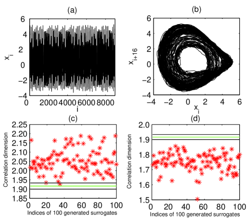
Figure 3: (a) Chaotic time series contaminated by observational noise ; (b) State space $x_{i+n}$ vs. $x_{i}$ of the chaotic time series from the Rössler system with $n=16$; (c) Surrogate test for the chaotic time series based on our new algorithm. The meaning of the lines and the curve is the same as that in panel $(c)$ of Fig. 1; (d) Surrogate test for the chaotic time series based on the PPS algorithm. The meaning of the lines and the asterisks is the same as that in panel $(c)$ of Fig. 1.

From Eq. (1) we see that the surrogates are generated from two segments $\{x_{i}\}_{i=1}^{N-\tau}$ and $\{x_{i+\tau}\}_{i=1}^{N-\tau}$ of the original time series $\{x_{i}\}_{i=1}^{N}$. We want segments $\{x_{i}\}_{i=1}^{N-\tau}$ and $\{x_{i+\tau}\}_{i=1}^{N-\tau}$ to equivalently affect the generation of the surrogates, therefore we would like to let $\max(\left|\alpha/\beta\right|)=\max(\left|\beta/\alpha\right|)$, $\min(\left|\alpha/\beta\right|)=\min(\left|\beta/\alpha\right|)$ and $\Pr(\left|\alpha/\beta\right|\geqslant 1)\simeq\Pr(\left|\beta/\alpha\right|\geqslant 1)$, where $\max(\cdot)$, $\min(\cdot)$ and $\Pr(\cdot)$ denote the maximal function, the minimal function and the probability function respectively. But note that the coefficient ratio $\alpha/\beta$ (or $\beta/\alpha$) shall not be too large or too small, otherwise $\left\{y_{i}^{\tau}\right\}$ will be very close to $\left\{x_{i}\right\}_{i=1}^{N-\tau}$ or $\left\{x_{i+\tau}\right\}_{i=1}^{N-\tau}$, which will lead to approximately the same correlation dimensions of $\left\{x_{i}\right\}_{i=1}^{N}$ and $\left\{y_{i}^{\tau}\right\}$ regardless of the dynamical behavior of $\left\{x_{i}\right\}_{i=1}^{N}$, and thus decrease the discriminating power of the correlation dimension. In our calculations we let $\alpha$ be uniformly drawn from the interval $\left[-0.8,-0.6\right]\cup\left[0.6,0.8\right]$ and $\beta=\sqrt{1-\alpha^{2}}$, which satisfies our requirements and provides moderate values for the ratio $\alpha/\beta$.

III Surrogate Test to Distinguish between Chaotic and Pseudoperiodic Time Series

In this section, through four examples from the Rössler system, we demonstrate the ability of surrogate test based on our algorithm to discriminate chaotic orbits from pseudoperiodic ones. As an application, we will also employ the surrogate technique to investigate whether a recorded human electrocardiogram (ECG) data set is possibly chaotic.

III.1 EXAMPLES

The equations of the Rössler system are given by

$$\left\{\begin{array}[]{l}\dot{x}=-y-z,\\ \dot{y}=x+ay,\\ \dot{z}=b+z(x-c).\end{array}\right.$$ (2)

with the initial conditions $x(0)=y(0)=z(0)=0.1$. We choose parameters $b=2$, $c=4$ and the sampling time $\Delta t_{s}$ $=0.1$ time units. For each example, the system is to be integrated $10,000$ times and the first $1,000$ data points are discarded to avoid including transient states.

In the first example, we set parameter $a=0.39095$. The Rössler system exhibits limit cycle behavior of period 6. To obtain pseudoperiodic time series, we introduce $5\%$ observational noise into the periodic time series. Although Gaussian white observational noise is the most common choice in this situation, in order to demonstrate the ability of our surrogate algorithm to deal with colored noise, we will instead adopt the noise generated from the $AR(1)$ process Box time (15) $\xi_{i+1}=0.8\xi_{i}+\epsilon_{i}$ with the variable $\epsilon$ following the normal Gaussian distribution $N(0,1)$, which is the more difficult case due to the correlation between noise components. However, one shall note that, Gaussian white noise and other colored noises satisfying the constraints in our null hypothesis, for example, those modelled by the $ARMA(p,q)$ processes, in principle can be dealt with in the same way. For convenience of observation and comparison, we plot the time series and the corresponding attractor in two dimensional state space (or embedding space) in panels $\left(a\right)$ and $\left(b\right)$ of Fig. 1 respectively.

To produce surrogate data, first we shall choose a suitable temporal translation. Since it is impractical to separate noise from signal completely, in general it is difficult to estimate the correlation decay time between noise components. Fortunately, to decorrelate noise components, all temporal translations are equivalent as long as they are large enough. In addition, in many real situations, it is often possible to observe the background noise and thus estimate the decay time. In our example, we think the $AR(1)$ noise to be uncorrelated when the temporal translation is larger than $50$ (in units of the sampling time $\Delta t_{s}$). As another requirement, temporal translation satisfying $cov(p_{i},p_{i+\tau})=0$ is desired. In practice, of course, this requirement is generally impractical due to the digitization and quantization in sampling process. Recall the discussion in the previous section, by letting $E(p_{i})=0$ and $\alpha^{2}+\beta^{2}=1$, we have $var(\alpha p_{i}+\beta p_{i+\tau})=var(p_{i})+2\alpha\beta\cdot cov(p_{i},p_{i+\tau})$. Function $cov(p_{i},p_{i+\tau})\neq 0$ means we do not preserve the noise level. However, under the null hypothesis of pseudoperiodicity, there shall always be some temporal translations to make $cov(p_{i},p_{i+\tau})\sim 0$, hence the noise level will not deviate from the original one too much. Besides, according to Eq. (1), we generate the surrogates by uniformly drawing coefficient $\alpha$ from interval $\left[-0.8,-0.6\right]\cup\left[0.6,0.8\right]$ ($\beta=\sqrt{1-\alpha^{2}}$ is always kept positive), the noise level of the surrogates will fluctuate around that of the original one due to the alternative signs of product $\alpha\beta$. Therefore, $cov(p_{i},p_{i+\tau})\neq 0$ will only cause some fluctuations when to calculate the correlation dimension because of the fluctuations of noise level, however, generally such fluctuations will not affect our conclusion if we can select a temporal translation $\tau$ to let $cov(p_{i},p_{i+\tau})\sim 0$. Since we have assumed the noise components are roughly independent of the deterministic components, then $cov(x_{i},x_{i+\tau})=cov(p_{i},p_{i+\tau})$ for a large enough temporal translation (to decorrelate noise components), therefore in all of the examples, in order to let $cov(p_{i},p_{i+\tau})\sim 0$, we can equivalently require $cov(x_{i},x_{i+\tau})\sim 0$. In the first example, there are many temporal translations satisfying the two constraints discussed above, i.e., $\tau>50$ and $cov(x_{i},x_{i+\tau})\sim 0$. To pick a value from all these candidates, we first select an interval $\left[100,150\right]$, then search the temporal translation which makes the absolute value $\left|cov(x_{i},x_{i+\tau})\right|$ be the minimum (most close to zero) among all translations $100\leqslant\tau\leqslant 150$. One shall note that the choice of the interval $\left[100,150\right]$ is arbitrary, except that we have to make sure that the lower bound of the interval is larger than $50$, and there exists temporal translations to let $cov(x_{i},x_{i+\tau})\sim 0$ within the interval. After selecting the temporal translation, by randomizing the coefficient $\alpha$ we will generate $100$ surrogates according to Eq. (1).

In order to calculate the correlation dimension, we adopt the time delay embedding reconstruction Takens detecting (16) to recover the underlying system from the scalar time series. Two parameters, i.e., embedding dimension and time delay, shall be properly chosen to apply this technique. Throughout this communication, we will use the false nearest neighbour criterion kernel determining (17) to determine the global optimal embedding dimension. Using the program in TISEAN package hegger practical (18), the embedding dimension $m$ of the original time series is selected at $4$, which is the minimal value to make the fraction of false nearest neighbours be zero. To choose a suitable time delay, we will use the algorithm of redundancy and irrelevance tradeoff exponent (RITE) proposed in Luo geometric (22). This algorithm selects the time delay by searching the optimal tradeoff between redundancy (due to too small time delay) and irrelevance (due to too large time delay). As demonstrated, the RITE algorithm can select equivalently suitable time delays compared to the average mutual information (AMI) criterion fraser and swinney independent (19), however, its implementation is much simpler and the computational cost is fairly low. Therefore in case of large data sets, adopting the RITE algorithm can facilitate our calculations. In the first example we generate $100$ surrogates, and for each surrogate we keep the embedding dimension $m=4$ and use the RITE algorithm to choose the suitable time delay for time delay reconstruction.

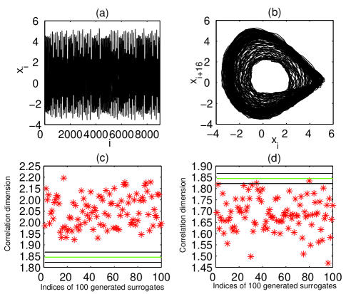
Figure 4: (a) Chaotic time series with both dynamical and observational noises; (b) State space $x_{i+n}$ vs. $x_{i}$ of the chaotic time series from the Rössler system with $n=16$; (c) Surrogate test for the chaotic time series based on our new algorithm. The meaning of the lines and the asterisks is the same as that in panel $(c)$ of Fig. 1; (d) Surrogate test for the chaotic time series based on the PPS algorithm. The meaning of the lines and the asterisks is the same as that in panel $(c)$ of Fig. 1.

We will follow Diks’s method Diks estimating (20) to calculate the correlation dimension, which is more robust against noise by extending the hard kernel function (or the Heaviside function) Grassberger characterization (13) in calculation of correlation integral to the general kernel functions. In his discussions, Diks adopted the Gaussian kernel function, hence this method is called Gaussian kernel algorithm (GKA). Here we will use the GKA implemented in Yu efficient (21) to calculate the correlation dimensions, which further enhances the computational speed. Note that to speed up the calculation, only 2000 data points are used as the reference points for the GKA. There are some statistical fluctuations even for the same data set when calculating its correlation dimension, therefore for the original time series, we will calculate $100$ times to estimate the mean correlation dimension and the standard deviation. As shown in panel $\left(c\right)$ of Fig. 1, there are three lines parallel to the abscissa. The middle line denote the estimation of the mean correlation dimension of the original time series, while the upper and lower lines indicate the positions twice the standard deviation away from the mean value. For the surrogates, however, we will calculate their correlation dimensions only once to save time. The results are illustrated as the asterisks in panel $\left(c\right)$ of Fig. 1.

After the calculation of the correlation dimensions, we need to inspect whether the result is consistent with our null hypothesis. Here we use the ranking criterion Theiler using (3) to determine whether the null hypothesis shall be rejected or not. The idea of this criterion is that, suppose the discriminating statistic of the original data set is $Q_{0}$, and those of $N_{S}$ surrogates are $\left\{Q_{1},Q_{2},~{}...,Q_{N_{S}}\right\}$. Rank the statistics $\left\{Q_{0},Q_{1},~{}...,Q_{N_{S}}\right\}$ in the increasing order and denote the rank of $Q_{0}$ by $r_{0}$, if the data set is consistent with the hypothesis (i.e., no evidence to reject), $r_{0}$ can have an equal possibility be any integer value between $1$ and $N_{S}+1$. However, if the hypothesis is false, $Q_{0}$ might deviate from the surrogate distribution $\left\{Q_{1},Q_{2},~{}...,Q_{N_{S}}\right\}$, i.e, $Q_{0}$ will be the smallest or largest amongst $\left\{Q_{0},Q_{1},~{}...,Q_{N_{S}}\right\}$, hence we can reject the null hypothesis if $r_{0}=1$ or $N_{S}+1$, the probability of a false rejection is $1/\left(N_{S}+1\right)$ for one-sided tests and $2/\left(N_{S}+1\right)$ for two-sided tests.

For the first example, from panel $\left(c\right)$ of Fig. 1 we can see that, the mean correlation dimension of the original time series falls within the dimension distribution of the surrogates, therefore we cannot reject the null hypothesis as we expect, which means the original time series is possibly pseudoperiodic note interpretation (23).

Now let us examine the other examples. In the second example, we still set parameter $a=0.39095$ in Eq. (2). However, to obtain the pseudoperiodic time series, we first generate a data set by adding Gaussian white noise with the standard deviation of $0.15\%$ to the $x$ component at each integration step, which simulates the system perturbed by additive dynamical noise, and then introduce $5\%$ observational $AR(1)$ noise into the previously obtained data set. The global optimal embedding dimension is chosen at $m=4$. Note in all of the four examples, we will generate $100$ surrogates, and parameter choices for surrogate generation will be the same, i.e., we let the temporal translation be selected from $\left[100,150\right]$ and coefficient $\alpha$ be uniformly drawn from $\left[-0.8,-0.6\right]\cup\left[0.6,0.8\right]$ ($\beta=\sqrt{1-\alpha^{2}}$). For the second example, the correlation dimensions of the original time series and the surrogates are shown in panel $\left(c\right)$ of Fig. 2. Under the ranking criterion, once again we cannot reject our null hypothesis. Therefore the time series is possibly pseudoperiodic, which is consistent with our knowledge.

In the third example, we change parameter $a$ of Eq. (2) to be $0.395$. The Rössler system exhibits chaotic behavior. We integrate Eq. (2) to obtain a time series and then introduce $5\%$ observational $AR(1)$ noise. The optimal embedding dimension $m$ is selected at $m=5$. From panel $\left(c\right)$ of Fig. 3, we find that the mean correlation dimension of the original time series deviates from the distribution of the surrogate dimensions. Using the ranking criterion, we can reject our null hypothesis. In order to exclude the possibility that the time series is generated from an unstable period orbit perturbed by dynamical noise, we also apply the PPS algorithm for further test. From the PPS algorithm we generate $100$ surrogates, and then use the GKA to calculate their correlation dimensions. The results are shown in panel $\left(d\right)$ of Fig. 3, as we can see, the mean correlation dimension of the original time series also falls outside the distribution of the surrogate dimensions, therefore we can reject the null hypothesis again. After the two surrogate tests for pseudoperiodicity, we can claim the time series is chaotic with a confidence level up to $96\%$ ($98\%\times 98\%$) for two-sided test.

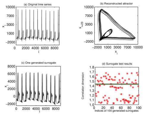
Figure 5: (a) Time series of a human electrocardiogram (ECG) record; (b) State space $x_{i+n}$ vs. $x_{i}$ of the ECG record with $n=23$; (c) A surrogate data generated from our algorithm with coefficient $\alpha=\beta=1/\sqrt{2}$ (cf. Eq. (1)); (d) Surrogate test for the ECG record based on our algorithm. The meaning of the lines and the asterisks is the same as that in panel $(c)$ of Fig. 1.

The final example to be demonstrated is a chaotic time series also from the Rössler system. To generate the time series, we keep parameter $a=0.395$. Similar to the way in the second example, we add Gaussian white noise with the standard deviation of $0.15\%$ to the $x$ component at each integration step as the dynamical noise, and then introduce $5\%$ observational $AR(1)$ noise into the previously obtained data set. The global optimal embedding dimension is found to be $m=4$. The results of surrogate tests based on the new algorithm and the PPS algorithm are shown in panel $(c)$ and $(d)$ of Fig. 4 respectively, from which we can see that, surrogate tests based on both algorithms can detect the chaos in the time series. Again we can claim the time series is chaotic with a confidence level up to $96\%$ for two-sided test.

We have also investigated examples under different observational noise levels (but keep the same dynamical noise if they have). For example, if we reduce the $AR(1)$ observational noise levels to $3\%$ in the above four examples, we can obtain the same results as we have reported. If we increase the observational noise levels to $10\%$, for the pseudoperiodic time series we can still obtain the expected results, i.e., we cannot reject our null hypothesis. However, for the chaotic time series, we will falsely accept our null hypothesis due to the correlation dimension of the original time series marginally falling within the dimension distribution of the surrogates. The reason of false acceptance might be that, under large noise levels, the correlation dimension is not sensitive enough to detect the structure changes of the chaotic time series. For such cases, we will have to look for more powerful discriminating statistics schreiber dircrimination (24).

III.2 AN APPLICATION

As an example of application, we employ the surrogate test based on our algorithm to investigate whether a human electrocardiogram (ECG) record (with $8975$ data points) is likely to be chaotic. The ECG record was obtained by measuring from a resting healthy subject ($22$ years old) in a shielded room at the sampling rate of $1$ KHz. The ECG record indicated in panel $(a)$ of Fig. 5 looks very regular and even possibly periodic, but we need a quantitative approach to verify the periodicity. Here we choose the surrogate test technique. Using the false nearest neighbour criterion, the global optimal embedding dimension is chosen at $m=5$. The background noise is mainly from the measurement instruments, usually it is a blend of white and correlated noise. By observing the linear second order correlation function of the ECG data, we let the temporal translation be within the interval $\left[100,150\right]$ (large enough to decorrelate the noise components), where there exists an integer temporal translation to make the correlation function almost be zero. Then by uniformly drawing values from $\left[-0.8,-0.6\right]\cup\left[0.6,0.8\right]$ for coefficient $\alpha$ in Eq. (1) ($\beta=\sqrt{1-\alpha^{2}}$ ), we generate $100$ surrogates. For demonstration, we plot in panel $\left(c\right)$ one surrogate generated from Eq. (1) with coefficient $\alpha=\beta=1/\sqrt{2}$. We can see that the surrogate is different from the original ECG data in that there appear more spikes in the surrogate. However, as we can also find, the surrogate indicates the similar regularity to that in the original data, which implies that the surrogate preserves the potential periodicity in the original data as we expect (although in a different pattern). With regards to the surrogate test, our calculation of the correlation dimensions is also based on the GKA. The results are indicated in panel $\left(d\right)$ of Fig. 5, from which we can see that the mean correlation dimension of the ECG data falls within the distribution of the correlation dimensions of the surrogates, therefore we cannot reject our null hypothesis. Hence the ECG record is possibly periodic. Moreover, there is no evidence of chaos.

IV Conclusion

To summarize, by imposing a few constraints on the noise process, we devise a simple but effective way to produce surrogates for pseudoperiodic orbits. The main idea of this algorithm is that a linear combination of any two segments of the same periodic orbit will generate another periodic orbit. By properly choosing the temporal translation between the two segments, under the same noise level we can obtain statistically the same correlation dimensions of the pseudoperiodic orbit and its surrogates. Choosing the temporal translation is a crucial issue for our algorithm, which in principle shall guarantee the decorrelation between the noise components and preserve the noise level. Another important issue is to select a proper discriminating statistic which helps determine whether to reject the null hypothesis. The correlation dimension is a suitable discriminating statistic in this case. It is possible there are other suitable discriminating statistics, we will leave the problem of finding such statistics for future study.

The surrogate test technique based on our algorithm can be utilized to distinguish between chaotic and pseudoperiodic time series. Initially, the PPS algorithm was proposed to generate surrogates for a pseudoperiodic orbit driven by dynamical noise, but sometimes surrogate tests based on this algorithm will falsely reject the null hypothesis if the time series is also contaminated by colored observational noise. As a complement to the PPS algorithm, our algorithm deals well with observational noise, but it might fail for large dynamical noise. However, due to the convenience in computation, we suggest to adopt surrogate test based on our algorithm as the first step for pseudoperiodicity detection. If we can reject the null hypothesis of our algorithm, then we shall use the PPS algorithm for further tests. If we can reject the null hypotheses of both the algorithms, then the time series under investigation is very likely to be chaotic. In this communication, the concrete procedures of surrogate test for pseudoperiodicity are demonstrated through four simulation examples. As an application in practice, we also employ the surrogate technique based on our algorithm to investigate whether a human ECG record is possible to be chaotic.

This research is supported by a Hong Kong University Grants Council Competitive Earmarked Research Grant (CERG) number PolyU 5235/03E.

References

- (1) J. Theiler, S. Eubank, A. Longtin, B. Galdrikian, and J.D. Farmer, Physica D 58, 77 (1992).
- (2) J. Theiler, Phys. Lett. A 196, 335 (1995).
- (3) J. Theiler and D. Prichard, Fields Inst. Commun. 11, 99 (1997).
- (4) A. Galka, Topics in Nonlinear Time Series Analysis with Implications for EEG Analysis (World Scientific, 2000).
- (5) Here we would like to elucidate that, the irregularity of a time series is usually brought by stochasticity or nonlinearity (often chaos), therefore in the example of nonlinearity detection, if we can exclude (most of) the probability that the time series is generated by a stochastic process, then it is very likely that the time series is generated from a nonlinear deterministic system.
- (6) D. Auerbach, P. Cvitanović, J.P. Eckmann, and G. Gunaratne, Phys. Rev. Lett. 58, 2387 (1987); P. Cvitanović, Phys. Rev. Lett. 61, 2729 (1988).
- (7) D. Pierson and F. Moss, Phys. Rev. Lett. 75, 2124 (1995); X. Pei and F. Moss, Nature (Lodon) 379, 618 (1996); P. So, E. Ott, S.J. Schiff, D.T. Kaplan, T. Sauer, and C. Grebogi, Phys. Rev. Lett. 76, 4705 (1996); P. Schmelcher and F.K. Diakonos, Phys. Rev. Lett. 78, 4733 (1997); K. Dolan, A. Witt, M.L. Spano, A. Neiman, and F. Moss, Phys. Rev. E 59, 5235 (1999).
- (8) D. Petracchi, Chaos, Solitons & Fractals 8, 327 (1997);
- (9) M. Small, D. Yu, and R.G. Harrison, Phys. Rev. Lett. 87, 188101 (2001).
- (10) For the definitions of the terminologies such as additive observational noise, please refer to Argyris the (11) for more details.
- (11) J. Argyris, I. Andreadis, G. Pavlos, and M. Athanasiou, Chaos, Solitons & Fractals 9, 343 (1998).
- (12) R. Quian Quiroga, A. Kraskov, T. Kreuz, and P. Grassberger, Phys. Rev. E 65, 041903 (2002).
- (13) P. Grassberger and I. Procaccia, Phys. Rev. Lett. 50, 346 (1983).
- (14) A. Jedynak, M. Bach, and J. Timmer, Phys. Rev. E 50, 1770 (1994).
- (15) G.E.P. Box, G.M. Jenkins, and G.C. Reinsel, Time Series Analysis: Forecasting and Control, 3rd Ed. (Prentice-Hall, 1994).
- (16) F. Takens, in D. Rand and L.S. Young, editors, Dynamical Systems and Turbulence (Springer, 1981).
- (17) M. B. Kennel, R. Brown, and H. D. I. Abarbanel, Phys. Rev. A 45, 3403 (1992).
- (18) R. Hegger, H. Kantz, and T. Schreiber, CHAOS 9, 413 (1999).
- (19) A. M. Fraser and H. L. Wwinney, Phys. Rev. A 33, 1134 (1986).
- (20) C. Diks, Phys. Rev. E 53, 4263 (1996).
- (21) D.J. Yu, M. Small, R.G. Harrison, and C. Diks, Phys. Rev. E 61, 3750 (2000).
- (22) X. Luo and M. Small (submitted, available from the URL: http://arxiv.org/abs/nlin.CD/0312023/).
- (23) We cannot claim the time series is pseudoperiodic definitely, because if we cannot reject a null hypothesis, there could be many interpretations other than that the data in test is consistent with our null hypothsis. For more details, see, for example, Ref. Galka topics (4).
- (24) T. Schreiber and A. Schmitz, Phys. Rev. E 55, 5443 (1997).