Static and Dynamic Correlations in Many-Particle Lyapunov Vectors

Abstract

We introduce static and dynamic correlation functions for the spatial densities of Lyapunov vector fluctuations. They enable us to show, for the first time, the existence of hydrodynamic Lyapunov modes in chaotic many-particle systems with soft core interactions, which indicates universality of this phenomenon. Our investigations for Lennard-Jones fluids yield, in addition to the Lyapunov exponent - wave vector dispersion, the collective dynamic excitations of a given Lyapunov vector. In the limit of purely translational modes the static and dynamic structure factor are recovered.

The dynamical instability of systems, which is quantified by the spectrum of Lyapunov exponents, has long been recognized as a most important characteristic for chaotic systems EckmannRuelle . Its understanding for extended dynamical systems provides essentials for the foundations of equilibrium and non-equilibrium statistical mechanics Dorfman . This explains the on-going scientific activities aiming at the connection between Lyapunov spectra of many-particle systems and macroscopic properties such as transport coefficients vBeijeren or entropy production rates DellagoPoschHoover96 ; ParingRulesEntropyProduction ; PoschForster . To each of the Lyapunov exponents in the spectrum one associates a Lyapunov vector in state or phase space, which in contrast to the Lyapunov exponent is a time-dependent quantity. Apart from singular early investigations Pomeau these mutually orthogonal vectors were for a long time used mainly as a means for calculating Lyapunov spectra. The scientific interest in these quantities raised when it was realized that especially in extended systems they contain non-trivial information about the perturbation dynamics. For instance, for certain coupled map lattices it was found that the Lyapunov vectors are often localized in state space LVlocalizedCML , a fact that was later also observed in many-particle systems LVlocalizedMPS ; ForsterHirschlPoschHoover ; PoschForster . Very recently, however, a very surprising phenomenon was observed. In contrast to the localized behavior of vectors belonging to the largest Lyapunov exponents, it was found that the Lyapunov vectors corresponding to near-zero exponents exhibit wave-like structures LVhydrodynamics ; ForsterHirschlPoschHoover ; PoschForster . Due to the approximately linear relation between Lyapunov exponent and wave number of the associated vector the latter were termed hydrodynamic Lyapunov modes. These findings immediately triggered theoretical efforts to gain deeper insights on the basis of simplified models such as products of random matrices LModeTheory . However, a really satisfactory state of understanding has not yet been achieved. For instance, molecular dynamics simulations indicated that hydrodynamic Lyapunov modes seem to exist only in hard-sphere or hard-disk fluids, but not in many-particle systems with soft interaction potentials LVhydrodynamics ; ForsterHirschlPoschHoover ; PoschForster . Although there are some arguments for this distinctive behavior based on fluctuations of finite time Lyapunov exponents, the existence of such a sharp difference between hard and soft potentials remains surprising. The purpose of this Letter is to show that hydrodynamic Lyapunov modes actually do exist also in soft-potential many-particle systems such as Lennard-Jones (LJ) fluids. This is achieved by considering static and dynamic correlation functions for the density of Lyapunov vector fluctuations, which we define appropriately in the spirit of generalized hydrodynamics GeneralizedHydrodynamics .

Before we present our results for Lennard-Jones fluids let us briefly recall the definition of Lyapunov vectors and their dynamics. For an autonomous dynamical system in $\mathbb{R}^{D}$ given by $\dot{\Gamma}=G(\Gamma)$ the tangent space dynamics describing small perturbation around a reference trajectory $\Gamma(t)$ is given by $\delta\dot{\Gamma}=M(\Gamma(t))\cdot\delta\Gamma$ with the Jacobian $M=\frac{dG}{d\Gamma}$. For a $D-$dimensional dynamical system there exist $D$ Lyapunov vectors $e^{(\alpha)}(t)\in\mathbb{R}^{D}$, $\alpha=1,\ldots,D$ which obey the equations of motion Goldhirsch ; HooverPoschBestiale

$$\dot{e}^{(\alpha)}=M(\Gamma(t))\cdot e^{(\alpha)}-\sum_{\beta=1}^{\alpha}m_{\alpha\beta}(t)~{}e^{(\beta)}$$ (1)

with $m_{\alpha\beta}(t)=\left[e^{(\alpha)}\cdot M(\Gamma(t))\cdot e^{(\beta)}+e^{(\beta)}\cdot M(\Gamma(t))\cdot e^{(\alpha)}\right]$ $\times(1-\delta_{\alpha\beta}/2)$. Eq.(1) describes the dynamics of a frame consisting of $D$ perturbation vectors $\delta\Gamma$ which are kept orthonormal by the nonlinear terms containing the Lagrange multipliers $m_{\alpha\beta}(t)$. The Lyapunov exponents $\lambda^{(\alpha)}$ are given by the time averages $\lambda^{(\alpha)}=\left\langle m_{\alpha\alpha}(t)\right\rangle_{t}$, with $\left\langle\ldots\right\rangle_{t}=\lim_{t\rightarrow\infty}\frac{1}{t}\int_{0}^{t}\ldots dt^{\prime}$. In practice one usually does not integrate Eq.(1) because of numerical instabilities, but rather obtains the Lyapunov vectors $e^{(\alpha)}(t)$ (and Lyapunov exponents) by the so-called standard method consisting of repeated Gram-Schmidt orthogonalization of an evolving set of $D$ perturbation vectors $\delta\Gamma(t)$ EckmannRuelle . One should note that with this procedure the Lyapunov vectors are automatically ordered such that $e^{(1)}$ belongs to the largest Lyapunov exponent $\lambda^{(1)}$, $e^{(2)}$ to the second largest $\lambda^{(2)}$, and so on. Eq.(1) corresponds to the continuum limit of this procedure and is given here explicitly to emphasize that $e^{(\alpha)}(t)$ is a well defined dynamical variable in continuous time.

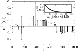
Figure 1: Snapshot of the LV density $u^{(\alpha)}(r,t)$ for a 1-d Lennard-Jones fluid ($N=100$) for which the corresponding Lyapunov exponent $\lambda^{(96)}$ is close to zero. The displacements $u_{i}^{(\alpha)}$ drawn vertically at the current particle positions $R_{i}$ show indications of a wave-like structure. The insert shows for this system the positive branch of the Lyapunov spectrum.

We treat the Hamiltonian dynamics of $N$ interacting particles of a $d-$dimensional fluid. Therefore $\Gamma=(R,P)$ is a phase space vector in $D=2dN$ dimensions evolving as $\Gamma(t)=\exp(i\mathcal{L}t)~{}\Gamma(0)$ where $\mathcal{L}$ denotes the Liouville operator. The coordinate part of $\Gamma$ is written as $R=(R_{1},\ldots,R_{N})$, with $R_{i}\in\mathbb{R}^{d}$ being the coordinate vector of the $i-$th particle. The momentum part $P$ is defined analogously. Correspondingly the Lyapunov vectors $e^{(\alpha)}$ can also be split into a coordinate and a momentum part as $e^{(\alpha)}=(u_{1}^{(\alpha)},\ldots,u_{N}^{(\alpha)},v_{1}^{(\alpha)},\ldots,v_{N}^{(\alpha)})$. In the following we will concentrate on correlations in the coordinate part of these vectors. For this purpose we introduce the dynamical variable $u^{(\alpha)}(r,t)=\sum_{i=1}^{N}u_{i}^{(\alpha)}(t)~{}\delta(r-R_{i}(t))$, which describes the spatial density of the coordinate part of Lyapunov vector fluctuations, which we call for short LV density. This variable is defined in analogy to other microscopic density fluctuations, e.g. of the particle current, in molecular hydrodynamics GeneralizedHydrodynamics . A snapshot of this dynamical variable is shown in Fig.1 for a 1-d LJ fluid. For translational invariant systems as treated here, it is convenient to consider the correlations of its Fourier transform $u^{(\alpha)}(k,t)=\int u^{(\alpha)}(r,t)~{}\exp(-ikr)~{}dr$ given by

$$u^{(\alpha)}(k,t)=\sum_{i=1}^{N}u_{i}^{(\alpha)}(t)~{}\exp(-ikR_{i}(t))$$ (2)

The intermediate two-time correlation function of this variable is defined as

$$F^{(\alpha\alpha)}(k,\tau)=N^{-1}\left\langle u^{(\alpha)}(k,t+\tau)~{}u^{(\alpha)}(-k,t)\right\rangle_{t}$$ (3)

which for $d\neq 1$ is a second rank tensor. From the latter we get for $\tau=0$ the static LV density correlation function $S^{(\alpha\alpha)}(k)=F^{(\alpha\alpha)}(k,\tau=0)$ and by Fourier transformation with respect to time the dynamical LV density correlation function $S^{(\alpha\alpha)}(k,\omega)=(2\pi)^{-1}\int F^{(\alpha\alpha)}(k,\tau)\exp(i\omega\tau)~{}d\tau$. Note that in contrast to the Lyapunov vectors itself, their correlation functions, being time averages, define global quantities similar to the Lyapunov exponents $\lambda^{(\alpha)}$. Even more far reaching is the following fact. It has been shown Ershov that generically for long times the Lyapunov vectors $e^{(\alpha)}(t)$ depend on time only via its current phase space point $\Gamma(t)$, especially it does not depend on the initial conditions $e^{(\alpha)}(t=0)$ as Eq.(1) might suggest. This implies that in long time averages $e^{(\alpha)}(t)$ can be replaced by $e^{(\alpha)}(\Gamma(t))$, where the vector fields $e^{(\alpha)}(\Gamma)$, $\alpha=1,\ldots,D$, provide what in Ershov is called a ”stationary Lyapunov basis”. Accordingly the evolution of the dynamical variables, e.g. Eq.(2), can be expressed as $u^{(\alpha)}(k,t)=\exp(i\mathcal{L}t)~{}u^{(\alpha)}(k,0)$ and, conceptually most important, the time averages in our correlation functions can be evaluated also as ensemble averages $F^{(\alpha\alpha)}(k,\tau)=N^{-1}\left\langle u^{(\alpha)}(k,t)~{}u^{(\alpha)}(-k,0)\right\rangle$ over the invariant density $\mu(\Gamma)$, i.e. $\left\langle\ldots\right\rangle=\int\ldots\mu(\Gamma)~{}d\Gamma$. Furthermore standard techniques for the analytical evaluation of these correlation functions, such as the Mori-Zwanzig projection operator formalism GeneralizedHydrodynamics , could be applied in principle. The problem, however, is the lack of knowledge about the vector fields $e^{(\alpha)}(\Gamma)$. One of the few known features is that for systems with translational invariance there exist Lyapunov vectors with constant spatial component $u_{i}^{(\alpha_{0})}=c^{(\alpha_{0})}$ belonging to the zero Lyapunov exponents $\lambda^{(\alpha_{0})}=0$ related to this symmetry LModeTheory . In these special cases the LV density variable $u^{(\alpha_{0})}(r,t)$ is proportional to the ordinary microscopic particle density $u^{(\alpha_{0})}(r,t)=c^{(\alpha_{0})}\rho(r,t)$ with $\rho(r,t)=\sum_{i=1}^{N}\delta(r-R_{i}(t))$ Mean . Correspondingly for these zero modes the components of the LV density correlation matrices $S^{(\alpha_{0}\alpha_{0})}(k)$ and $S^{(\alpha_{0}\alpha_{0})}(k,\omega)$ are simply proportional to the static and dynamic structure factor $S(k)$ and $S(k,\omega)$, respectively.

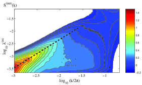
Figure 2: Contour lines of the static correlation functions $S^{(\alpha\alpha)}(k)$ for a 1-d Lennard-Jones fluid ($N=100$, $L=1000$, $T=0.2$) plotted as function of $k$ and $\lambda^{(\alpha)}$. The ridge at low $k-$ and $\lambda-$values as indicated by the dashed line, implies the existence of hydrodynamic Lyapunov modes.

The general behavior of $S^{(\alpha\alpha)}(k)$ and $S^{(\alpha\alpha)}(k,\omega)$ is inferred from numerical simulations. The particle dynamics is obtained by integrating Hamilton’s equations with periodic boundary conditions using a standard truncated LJ interaction potential given by $V(r)=4\epsilon[(\sigma/r)^{12}-(\sigma/r)^{6}]-V_{c}$ for $r<r_{c}=2.5\sigma$ and $V(r)=0$ elsewhere Kob . $V_{c}$ is chosen such that $V(r)$ is continuous at $r_{c}$, and the parameters $\sigma$, $\epsilon$ and the particle mass $m$ are all set to unity. This means that e.g. system length $L$, (kinetic) temperature $T$ and time is measured in units of $\sigma$, $\epsilon$, and $(m\sigma^{2}/48\epsilon)^{1/2}$, respectively. The Lyapunov vectors $e^{(\alpha)}(t)$ were obtained iteratively with the standard method EckmannRuelle . The time step used in the symplectic Verlet algorithm of our MD simulations is $\Delta=0.008$ and the re-orthogonalization for the calculation of the $e^{(\alpha)}(t)$ is repeated in time intervals of $30-100\Delta$. The numerical evaluation of the correlation functions is started only after appropriate equilibration periods. The coordinate part of a Lyapunov vector, as shown in Fig.1 for $L=1000$ and $T=0.2$ is a quantity fluctuating in space and time. The equal time correlations in space are captured by $S^{(\alpha\alpha)}(k)$. For simplicity we present first results for the one-dimensional LJ fluid, for which $S^{(\alpha\alpha)}(k)$ is a scalar quantity. In this case we can depict its behavior in a contour plot. Since for $\lambda^{(\alpha)}>0$ the latter decreases monotonically with the index $\alpha$, we can plot $S^{(\alpha\alpha)}(k)$ also over the $\lambda-k-$plane thereby introducing the function $S(\lambda,k)$. The surmise, which is supported by our numerical simulations, is that the latter converges with increasing $N$ (for fixed temperature $T$ and density $N/L$) to a well-defined limit. In the contour plot of Fig.2 we recognize a ridge at small $\lambda$ and $k$, which defines a dispersion relation $\lambda(k)$ or $k(\lambda)$ implying that the Lyapunov mode corresponding to Lyapunov exponent $\lambda$ is dominated by a spatial oscillation with wave number $k(\lambda)$. In Fig.3 we determined the dispersion relation $\lambda(k)$ by plotting $\lambda$ versus $k_{\max}=\arg\max_{k}S(\lambda,k)$ for various systems differing in density and temperature. We find that the dispersion $\lambda(k)$ appears to be independent of these parameters in the regions where $\lambda(k)$ is well defined. Only the extent of the latter regions is parameter dependent, as it decreases e.g. with decreasing density. The common dispersion relation $\lambda(k)$ being linear on a log-log scale results in a power law $\lambda(k)\sim k^{\eta}$ with $\eta=1.2\pm 0.1$ although a linear dispersion with quadratic corrections cannot be excluded. In any case these results unambiguously show the existence of hydrodynamic Lyapunov modes in LJ fluids. Actually, our investigations show that their existence is not restricted to 1-d systems. In isotropic fluids with $d>1$ the Cartesian components $F_{\mu\nu}^{(\alpha\alpha)}(k,\tau)$ of $F^{(\alpha\alpha)}(k,\tau)$ can be written in terms of longitudinal and transverse correlation functions $F_{L}^{(\alpha\alpha)}$ and $F_{T}^{(\alpha\alpha)}$ as $F_{\mu\nu}^{(\alpha\alpha)}(k,\tau)=\hat{k}_{\mu}\hat{k}_{\nu}F_{L}^{(\alpha\alpha)}(\left|k\right|,\tau)+(\delta_{\mu\nu}-\hat{k}_{\mu}\hat{k}_{\nu})F_{T}^{(\alpha\alpha)}(\left|k\right|,\tau)$ with $\hat{k}_{\mu}=(k/\left|k\right|)_{\mu}$. We find for $d=2$ that $F_{L}^{(\alpha\alpha)}(\left|k\right|,0)$ and $F_{T}^{(\alpha\alpha)}(\left|k\right|,0)$ behave similar to the 1-d case shown in Fig.2 implying the existence of hydrodynamic Lyapunov modes also there.

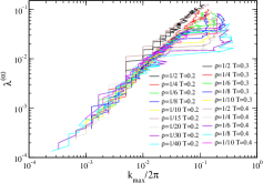
Figure 3: The dispersion relation $\lambda(k)$ of the hydrodynamic Lyapunov modes shown for different particle densities and temperatures, appears to be independent of the latter for a wide range of parameters.

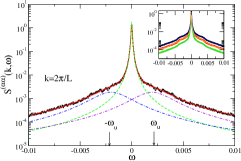
Figure 4: The dynamic correlation function $S^{(\alpha\alpha)}(k,\omega)$ for $\alpha=96$ and $k=2\pi/L$. The full line results from a fit by a 3-pole approximation. The corresponding decomposition into three Lorentzians is also shown. The insert shows a comparison of such fits for $k=2\pi/L$, $4\pi/L$, and $8\pi/L$ (from the top).

More detailed information can be obtained from the dynamical LV correlation functions $S^{(\alpha\alpha)}(k,\omega)$, which encode in addition to the structural also the temporal correlations. As usual the equal time correlations can be recovered by a frequency integration $S^{(\alpha\alpha)}(k)=\int S^{(\alpha\alpha)}(k,\omega)~{}d\omega$. In Fig.4 we show typical examples for $S^{(\alpha\alpha)}(k,\omega)$. It consist of a central ”quasi-elastic” peak with shoulders resulting from dynamical excitations quite similar to the dynamical structure factor $S(k,\omega)$ of fluids. In order to extract the dynamical information we used a 3-pole approximation for the Laplace transform of $F^{(\alpha\alpha)}(k,\tau)$ from Eq.(3), which amounts to fitting $S^{(\alpha\alpha)}(k,\omega)$ by a superposition of three Lorentzians, one central peak at $\omega=0$ and two symmetric peaks located at $\omega=\pm\omega(k)$. The fits are also shown in the figure and describe the frequency dependence of $S^{(\alpha\alpha)}(k,\omega)$ quite well. Such a dependence arises naturally e.g. from continued fraction expansions based on Mori-Zwanzig projection techniques GeneralizedHydrodynamics , which as mentioned may be applied also to this problem. These fits allow us to extract the dispersion relations $\omega^{(\alpha)}(k)$ for each of the hydrodynamic Lyapunov modes with index $\alpha$. The result is shown in Fig.5 for several of the Lyapunov modes. Clearly, this tells us that a Lyapunov mode corresponding to exponent $\lambda$ is characterized, apart from the dominating wave length $k(\lambda)$, by a typical frequency $\omega(k(\lambda))$. Because $\frac{d\omega}{dk}$ is non-vanishing, this implies propagating wave-like excitations. The origin of the characteristic frequency $\omega(k(\lambda))$ is not yet fully understood. Probably it reflects rotational motion of the orthogonal frame $\left\{e^{(\alpha)}(t)\right\}$ around its reference trajectory PoschForster . The full LV dynamics, however, is more complex. We find, for instance, that the coherent wave-like motion is switched on and off intermittently YangRadons . This phenomenon presumably is responsible for the strong central peak in $S^{(\alpha\alpha)}(k,\omega)$ (see Fig.4).

In summary, we have shown that the LV density correlation functions provide a valuable tool for quantifying spatiotemporal phenomena in many-particle Lyapunov vectors. They allowed us to identify for the first time hydrodynamic Lyapunov modes and their dynamics in soft-potential systems. These findings indicate that the existence of hydrodynamic Lyapunov modes is a universal phenomenon in chaotic translation invariant many-particle systems, independent of the interaction potential. This view is supported by the fact that these modes appear to be present also in one- and two-dimensional fluids with Weeks-Chandler-Anderson (WCA) interaction potentials PoschPriv . There exist obvious generalizations of our correlation functions, which will be treated in forthcoming papers. For instance, one can consider correlations between different Lyapunov vectors resulting in cross-spectra $S^{(\alpha\beta)}(k,\omega)$, or correlations of the LV density not only in coordinate space but in phase space $e^{(\alpha)}(r,p,t)=\sum_{i=1}^{N}e_{i}^{(\alpha)}(t)~{}\delta(r-R_{i}(t))\delta(p-P_{i}(t))$, which is an approach used similarly in kinetic theory GeneralizedHydrodynamics .

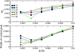
Figure 5: Dispersion relations $\omega^{(\alpha)}(k)$ (top) and the $k-$dependence of the width of the central peak (bottom) for different Lyapunov vectors obtained from 3-pole approximations as in Fig.4. Note the clear separation of the corresponding time scales.

Acknowledgments

We thank H. Posch, A. Pikovsky, W. Just, A. Latz, and especially W. Kob for illuminating discussions. Support from the Deutsche Forschungsgemeinschaft within the SFB 393 ”Numerische Simulation auf massiv parallelen Rechnern” is gratefully acknowledged.

References

- (1) J.-P. Eckmann, D. Ruelle, Rev. Mod. Phys. 57, 617 (1985); E. Ott, Chaos in Dynamical Systems (Cambridge University Press, Cambridge 1993).
- (2) J.R. Dorfman, An Introduction to Chaos in Nonequilibrium Statistical Mechanics. (Cambridge University Press, Cambridge, 1999); P. Gaspard, Chaos, Scattering and Statistical Mechanics. (Cambridge University Press, Cambridge, 1998).
- (3) H. van Beijeren and J. R. Dorfman, Phys. Rev. Lett. 74, 4412 (1995); H. van Beijeren et al, Phys. Rev. Lett. 77, 1974 (1996); R. van Zon, H. van Beijeren, and Ch. Dellago, Phys. Rev. Lett. 80, 2035 (1998); P. Gaspard et al, Nature 394, 865 (1998), C. P. Dettmann, E. G. D. Cohen, and H. van Beijeren, Nature 401, 875 (1999), C. P. Dettmann, E. G. D. Cohen, J. Stat. Phys. 103, 589 (2001), P. Gaspard and H. van Beijeren, J. Stat. Phys. 109, 671 (2002).
- (4) Ch. Dellago, H. A. Posch, and W. G. Hoover, Phys. Rev. E 53, 1485 (1996).
- (5) C. P. Dettmann and G. P. Morriss, Phys. Rev. E 53, R5545 (1996), F.Bonetto, E.G.D. Cohen, and C.Pugh, J. Stat. Phys. 92, 587 (1998), E. G. D. Cohen and L. Rondoni, Chaos 8, 357 (1998), D.Ruelle, J. Stat. Phys. 95, 393 (1999), H. van Beijeren and J. R. Dorfman, Physica A 279, 21 (2000), D. Panja, J. Stat. Phys. 109, 705 (2002), Tooru Taniguchi and Gary P. Morriss, Phys. Rev. E 66, 066203 (2002).
- (6) H.A. Posch, Ch. Forster, in Collective Dynamics of Nonlinear and Disordered Systems, p.309, Eds. G. Radons, W. Just, and P. Häussler (Springer, Berlin, 2004), in print.
- (7) Y. Pomeau, A. Pumir, and P. Pelce, J. Stat. Phys. 37, 39 (1984), K. Kaneko, Physica D 23, 436 (1986).
- (8) G. Giacomelli, A. Politi, Europhys. Lett. 15, 4387 (1991), H. Chate, Europhys. Lett. 21, 419 (1993), A. Pikovsky, A. Politi, Nonlinearity 11, 1049 (1998), A. Pikovsky, A. Politi, Phys. Rev. E 63, 036207 (2001).
- (9) Lj.Milanović, H.A.Posch, and Wm.G.Hoover, Chaos 8, 455 (1998), Tooru Taniguchi and Gary P. Morriss, Phys. Rev. E 68, 462031 (2003).
- (10) Ch. Forster, R. Hirschl, H.A. Posch, W. G. Hoover, Physica D 187, 294 (2004).
- (11) Lj.Milanović, H.A.Posch, and Wm.G.Hoover, Molec. Phys. 95, 281 (1998), H. A. Posch and R. Hirschl, in Hard ball systems and the Lorentz gas, p.269, EMS Vol. 101, Ed. D. Szasz (Springer, Berlin, 2000), Wm.G. Hoover et al, J. Stat. Phys. 109, 765 (2002).
- (12) J.-P. Eckmann, O. Gat, J. Stat. Phys. 98, 775 (2000), S. McNamara, M. Mareschal, Phys. Rev. E 64, 051103 (2001), Tooru Taniguchi and Gary P. Morriss, Phys. Rev. E 65, 056202 (2002), M. Mareschal, S. McNamara, Physica D187, 311 (2004).
- (13) J. P. Hansen and I. R. McDonald, Theory of Simple Liquids, 2nd ed. (Academic Press, London, 1990).
- (14) I. Goldhirsch, P.-L. Sulem, and S.A. Orszag, Physica D 27, 311 (1987).
- (15) W.G.Hoover, H.A.Posch, and S. Bestiale, J. Chem. Phys. 87, 6665 (1987).
- (16) S.V. Ershov and A.B. Potapov, Physica D 118, 167 (1998).
- (17) In these cases the dynamical variables have non-vanishing mean values which have to be subtracted before the correlation functions are formed.
- (18) The core of our molecular dynamics program is an adaptation of the code provided to us by Walter Kob and used e.g. in W.Kob and H.C. Andersen, Phys. Rev. E 51, 4626 (1995).
- (19) Hongliu Yang and G. Radons, Lyapunov instability of Lennard Jones fluids, Phys. Rev. E, submitted.
- (20) H.A. Posch, talk given at DPG-Frühjahrstagung, Regensburg, 8-12 March 2004, Ch. Forster and H.A. Posch, in preparation.